Article

Joint Decisions of Inventory Optimization and Order Allocation for Omni-Channel Multi-Echelon Distribution Network

1
GBA and B&R International Joint Research Center for Smart Logistics, Jinan University, Zhuhai 519070, China
2
School of Intelligent Systems Science and Engineering, Jinan University, Zhuhai 519070, China
3
Institute of Physical Internet, Jinan University, Zhuhai 519070, China
4
School of Management, Jinan University, Guangzhou 510632, China
5
College of Mathematics and Informatics, South China Agricultural University, Guangzhou 510642, China
6
Department Industrial and Manufacturing Systems Engineering, The University of Hong Kong, Hong Kong, China
*
Author to whom correspondence should be addressed.
Sustainability 2022, 14(10), 5903; https://doi.org/10.3390/su14105903
Submission received: 26 March 2022 / Revised: 4 May 2022 / Accepted: 6 May 2022 / Published: 13 May 2022
(This article belongs to the Special Issue Logistics and Sustainable Supply Chain Management (Series) II)

Abstract

:
Firms with omni-channel multi-echelon distribution networks (OMDC) integrate all of their sale channels and distribution echelons to achieve an effective matching of multi-type orders and a shared inventory. However, the high operational cost caused by insufficient use of inventory resources and unreasonable order allocation restricts the sustainable development of firms. To this end, the joint decisions of inventory optimization (IO) and order allocation (OA) are explored to achieve cost-efficient and sustainable omni-channel operations. Specifically, from the perspective of IO, an inventory integrated policy is proposed for online and offline inventory sharing within nodes and lateral transshipment between nodes; from the aspect of OA, an order allocation mechanism is designed for the minimum cost under the influence of multiple factors (inventory replenishment, holding, order delivery distance and time) among different echelon nodes. A joint optimization model of an inventory and orders is therefore developed and is subsequently solved using the Genetic Algorithm (GA). Results obtained show that the proposed strategy has a better performance with regards to operational cost and customer service level and is also more sustainable than alternative strategies. The proposed joint strategy provides a relatively novel approach to realize flexible and sustainable omni-channel distribution systems.

1. Introduction

Sustainability is an important topic for the world today, and incorporating sustainability practices into supply chain networks has attracted wide attention from the industry and academia [1]. Sustainable supply chains emphasize that while coordinating the critical organizational business for improving the long-term financial performance, supply chain participants are requested to achieve the organization’s social, environmental and economic goals [2]. Therefore, in addition to considering economic goals of cost reduction and profit increase, firms should also take social and environmental performance into account [3], including customer well-being, energy consumption and emissions, when making management decisions in order to achieve sustainable development.
With the development of information technologies and the popularity of e-commerce, most commodity distribution firms, especially firms with multi-echelon distribution networks, retained the traditional offline distribution channels while establishing online channels, forming a dual-channel distribution mode with the coexistence of online and offline channels [4,5], where each channel has separate inventory, operation system and commercial teams [6]. Although this decentralized management can broaden the sale approaches to some extent, it often leads to a higher operational cost, an overall increase in inventory and a decrease in operational efficiency and customer service level [6,7,8], which are caused by the following two aspects. Firstly, each node of the network mostly holds an online and offline independent inventory rather than a shared inventory to meet customers’ online and offline needs, increasing the holding cost and wasting the inventory resources [6]. Secondly, the proximity-based assignment principle of online orders allows excessive orders to be pooled in the lower echelon nodes of the distribution network (for example, stores), which not only exacerbates the risk of stock-outs at the lower nodes [9] but also causes firms to replenish inventory by increasing the frequency of replenishment, causing the waste of transportation resources and increasing the emissions [10]. Moreover, the consideration of the second aspect will in turn affect the inventory of each node in the first aspect. As a result, there is an urgent need for firms to seek new modes to pursue sustainable development.
Recently, the omni-channel distribution mode has increasingly attracted the attention of many scholars because it can provide customers with consistent goods and services by effectively integrating inventory, customer and other information data from all sales channels [11,12]. For this mode, optimizing the above-mentioned inventory and online order allocation problems will, on the one hand, enable the firm to integrate the resources of various channels to reduce operational costs and thus provide customers with high service and quality products, improve customer satisfaction and increase sales profits [13], thus achieving economic sustainability; on the other hand, the firm will reduce land occupation by reducing inventory holdings and reduce the emissions by optimizing the order fulfillment mode [14], thus achieving environmental sustainability. Therefore, it is of great importance for firms with multi-echelon distribution networks to make joint decisions of inventory optimization (IO) and order allocation (OA) in omni-channel.
For the IO in multi-echelon distribution networks, there is an increasing number of studies focusing on the methods of online and offline inventory sharing within nodes (referred to as inventory sharing) and lateral transshipment between nodes [15,16,17,18]. The inventory-sharing method aims to achieve optimal system-wide holdings at a given service level by integrating online and offline inventory [19], which can reduce the overall inventory level within nodes but cannot avoid the risk of its own stock-outs. The lateral transshipment method refers to stock movements between nodes in the same echelon of the supply chain network by transshipping the available inventory of one node to meet the shortage at another node [20], which prevents the loss of offline orders of store nodes and is also environmentally friendly [21]. However, most of the existing research has focused on one or the other, while it is still relatively rare to integrate inventory sharing and lateral transshipment to optimize inventory level in omni-channel multi-echelon distribution networks (OMDN).
As for OA in multi-echelon distribution networks, current studies have focused on the issue of the selection of fulfillment node for each order [9,22,23]. The existing studies find that the selection of upper echelon nodes can reduce the unit inventory cost and replenishment frequencies but increase the order delivery time and return risk due to the longer delivery distance; while the selection of lower echelon nodes can reduce the order delivery distance and time but increase the unit inventory cost and replenishment cost. Currently, although there is some existing literature exploring the way of order allocation, the studies about how to integrate multi-dimensional factors related to order fulfillment costs among different echelon nodes in OMDN, including the inventory replenishment, holding, order delivery distance and time to achieve optimal order allocation is less common.
More importantly, while the issues of IO and OA relate to the storage and transportation of goods and have a significant impact on the sustainability of the supply chain [10], there is little literature on the exploration of both in an omni-channel multi-echelon and multi-node network.
To address the above-mentioned research gaps, we innovatively propose a joint model of inventory optimization and order allocation for OMDN, aiming to achieve cost-efficient and sustainable omni-channel operations. Firstly, from the perspective of IO, an inventory integrated policy is explored for online and offline inventory sharing within nodes and lateral transshipment between nodes; from the aspect of OA, an order allocation mechanism is designed for the minimum cost under the influence of multiple factors (inventory replenishment, holding, order delivery distance and time) among different echelon nodes of the network. Then, a joint optimization model is developed and solved by genetic algorithm (GA). Finally, based on an example analysis, the effectiveness of the proposed inventory and order allocation strategy is verified by comparing the alternative strategies and more insights are showed on the analysis of the system parameters.

2. Literature Review

This section will review the literature on inventory optimization policies and online order allocation and fulfilment issues, as these are not only relevant to our paper, but are two important aspects that affect the efficiency and sustainability of omni-channel operations as well as customer satisfaction.

2.1. Omni-Channel and Inventory Optimization Policy

Omni-channel is a relatively new area in the e-commerce supply chain which has received widespread attention. Omni-channel refers to the integration of multiple sales channels to seamlessly meet the diverse needs of customers; it was first introduced by Rigby [24] and has subsequently been further expanded by many scholars in different dimensions [11,12,25]. A large body of literature focuses on omni-channel operational modes and consumer behavior. Taylor et al. [26] summarized six omni-channel operational modes including BOPS and STS through empirical analysis. Gallino and Moreno [25] explored the impact of consumer transfers on omni-channel retailing through an empirical study. In addition, the integration of various factors between online and offline channels, including inventory and order information, is also an important aspect of omni-channel operations.
Early in the development of e-commerce, Seifert et al. [27] explored the integration between virtual stores and existing supply chains. With the emergence of online channels, Herhausen et al. [28] examined the impact of online and offline channel integration and showed that retailers can create competitive advantage through channel integration. Mahar et al. [29] investigated the virtual integration of inventory information across nodes in dual-channel to achieve a significant reduction in system costs. Alawneh and Zhang [6] demonstrated that the existence of an integrated dual-channel warehouse can increase flexibility. With the development of omni-channel, Saghiri et al. [30] constructed a three-dimensional framework model consisting of consumer purchasing process, channel type, and channel agent, emphasizing effective integration between each stage of omni-channel. From the existing literature about omni-channel, qualitative research is more common while quantitative research is lacking, especially on inventory integration of online and offline channels, for which this paper will focus on.
In addition, the inventory transshipment policy has proven effective in reducing inventory levels across supply chain networks [31]. Paterson et al. [20] provided a detailed review of recent studies on quantitative lateral transshipment. In the traditional offline sales, Ahmadi et al. [32] developed a location-inventory model in a three-echelon distribution network using a proactive transshipment. Firoozi et al. [33] proposed a two-stage stochastic model to optimize inventory decisions by considering lateral transshipment and multi-sourcing strategies. For the e-commerce retailing, Torabi et al. [22] proposed a Benders decomposition algorithm to select order fulfillment nodes and make transshipment decisions. In multi-channel, Zhao et al. [18] adopted lateral transshipment in online-to-offline supply chain to reduce inventory risk due to demand uncertainty. Fan et al. [34] investigated the impact of considering customer transfer and inventory transshipment on optimal inventory levels and costs in a two-channel supply chain. Derhami et al. [35] considered inventory transshipment and product substitution in an omni-channel supply chain network and demonstrated that inventory transshipment can improve customer satisfaction. The above literature shows that the inventory transshipment policy is now widely used in supply chains and has been explored to some extent in omni-channel mode. However, the integration of online and offline inventory within nodes and lateral transshipment between nodes to simultaneously optimize inventory level in a multi-echelon distribution network has been less commonly discussed.

2.2. Order Allocation and Fulfillment

The allocation decision of online orders has enjoyed much attention in recent years. Agatz et al. [36] proposed that the optimal order allocation issue is an emerging problem nowadays. Most literature is currently available on the assignment of online orders based on the proximity principle. For example, Torabi et al. [22] considered the allocation of orders on the basis of the closest distance in an e-retail environment with the goal of minimizing transportation costs. Acimovic and Graves [37] developed a heuristic model to optimally allocate each online order to minimize the distribution cost. Govindarajan et al. [23] firstly allocated online orders to the closest nodes and considered the order transfer when the nodes are out-of-stock to minimize delivery and penalty costs in an omni-channel network. However, the allocation of online orders which only consider the delivery distance does not mean the total profit of the network is maximized [38]. Building on Govindarajan et al. [23], DeValve et al. [39] set an abandoning probability to restrict order transfer to reformulate the order optimal allocation decision. The existing studies have failed to explore more factors affecting the optimal allocation decision of orders.
There is also a large number of studies that explore the different ways retailers fulfill customer orders. Ishfaq and Bajwa [40] classified the way order fulfillment into the following 3 options: (1) dedicated fulfillment centers for online orders; (2) stores, which fulfill part of the online demand while mainly satisfying offline customers; (3) distribution centers, which add the function of shipping online orders while mainly providing replenishment for lower echelon nodes. There is a wealth of research considering dedicated fulfillment centers as well as physical stores to fulfill online orders. Chen et al. [41] studied how to allocate and fulfill the orders in a supply chain network consisting of an online retailer and two brick-and-mortar retailers. Ali et al. [42] proposed a multi-objective mixed integer planning model to satisfy online orders from stores or fulfillment centers. Alishah et al. [43] made the optimal cross-channel fulfillment decision in a supply chain consisting of a retail stores and a fulfillment center. Moreover, there is literature exploiting the existing facilities to study the order fulfillment problem. For example, Alawneh and Zhang [6] investigated how existing warehouses assign and satisfy both online and offline demand. Liu et al. [19] also considered the allocation of online demand to regional warehouses that originally met in-store demand in a multi-channel. In particular, store fulfillment has received widespread attention given its advantages of proximity to customers and short delivery distance and time [23,44,45]. However, the network structures considered in the above work are mostly single- or two-echelon, and fewer studies consider order fulfillment issue in a multi-echelon and multi-node.
Although a large number of studies have been conducted, respectively, on inventory optimization policies and online order allocation, the joint study of these two issues as an omni-channel multi-echelon distribution network has received less consideration. Thus, this paper studies the joint optimization problem of inventory and order allocation in a multi-echelon and multi-node network by facing both online and offline uncertain demands, designing the inventory integration policy of inventory sharing within nodes and lateral transshipment between nodes, and the order allocation mechanism for the minimum cost under the influence of multiple factors, to enrich the related studies about the omni-channel field.

3. Problem Description and Modelling

This section will describe the problem context and then develop a joint optimization model.

3.1. Problem Description

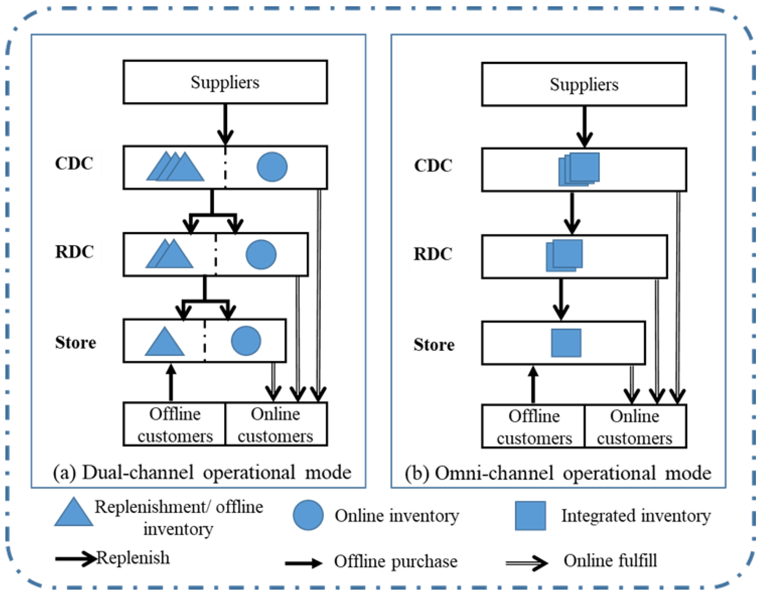
This paper considers a three-echelon distribution network of a B&M firm in mainland China, consisting of external suppliers, a set of central distribution centers (CDCs), regional distribution centers (RDCs) and stores. As illustrated in Figure 1a, each echelon node holds two types of inventory and is replenished by their upper nodes; and suppliers out the scope of the paper are mainly for supplying to the CDCs. An operational time horizon is considered (for example, weekly, monthly) and is divided into a set of control periods (for example, daily). At a given period, the network faces offline demand from consumers purchasing in stores, which is met by offline inventory in stores; and it also faces online demand from consumers ordering online, which is collected at a certain time point and then satisfied by the online inventory of the closest node to the customer (including CDCs, RDCs and stores). Unmet offline and online demand is accounted for as out-of-stock losses. In addition, the replenishment demand from RDCs and stores are responded to by the replenishment inventory of the CDCs and RDCs. However, in this dual-channel mode, the online and offline inventory in the nodes operate independently, and online orders are assigned to the closest nodes, which often leads to the problem of high inventory holding at each node and high order fulfillment costs between distribution networks. Therefore, how to optimally manage the inventory at each node and optimally allocate the online orders to reduce the total cost of the distribution network is an urgent issue to be solved.
This paper proposed an inventory integration policy of inventory sharing within nodes and lateral transshipment between nodes from the perspective of IO. As illustrated in Figure 1b, the online and offline replenishment inventory at each node is integrated into one type of inventory and replenished by upper echelon nodes. Moreover, when the inventory of a store is unavailable, it can request lateral transshipment from other stores. An order allocation mechanism for the minimum cost under the influence of multiple factors is adopted from the aspect of OA: the online orders are assigned to the node with minimum cost affected on replenishment cost, inventory holding cost, order delivery cost, and time penalty cost for the loss of some online orders due to longer order delivery time.
Given the above inventory and order joint strategy, we will answer the following questions at each decision opportunity: (1) the optimal allocation node for online orders in each period; (2) the optimal inventory replenishment amount for each node in each period; (3) the optimal inventory transshipment amount in case of insufficient inventory in store nodes in each period.

3.2. Problem Assumptions and Parameter Definitions

The notation of the parameters used in the model in this paper is shown in Table 1 and the problem assumptions are given as follows:
(1)
A single kind of product with the same quality and price is considered;
(2)
The online and offline demands of each node are stochastic and independent and follow a normal distribution;
(3)
Each node adopts a periodic review policy and the replenishment between different echelons had the lead time;
(4)
Each node has a different distribution region, and the distribution region between nodes of the same echelon does not overlap, and between different echelon nodes the upper nodes will cover the whole region of lower replenishment nodes;
(5)
We measure the location and the shortest delivery time of online customers by the closest node in the distribution range and choose the node with minimum cost within distribution networks to fulfill online orders;
(6)
Except suppliers, each echelon node in the distribution network has the inventory capacity limit;
(7)
Lateral transshipments are only conducted after the realization of actual demands: we adopt an emergency transshipment policy;
(8)
For offline orders, it only occurs stock-out when the store node requests lateral transshipment and still cannot be satisfied; for online orders, it occurs stock-out only when the node whose total cost including the stock-out cost is still the lowest. The loss will be calculated at that node.

3.3. The Omni-Channel Multi-Echelon Joint Optimization Model

In this paper, we study the joint problem of inventory optimization and order allocation for OMDN, which can be described as follows: for each period t and known online and offline demand in OMDN with a set of CDCs (w), RDCs (u) and stores (k), making joint decisions of the allocation node for online orders, the replenishment amount of each node and the transshipment node and amount between store nodes to minimize the total cost in OMDN.
Based on the inventory optimization model in Firoozi et al. [33], the model of this paper is formulated as follows:
Minimise:
m i n T C = t T ( T C K + T C U + T C W ) .  
With respect to:
z n n t ,   n = n   { w , u , k } ;   Q n n t , n = { s , w , u } ,   n = { w , u , k } ;   y n n t , n = { k }
where:
T C K = C R K + C T K + C H K + C F K + C S K = t T k K ( g k Q u k t + k K c k k d k k y k k t + h k / 2 ( I k , t 1 + + Q u k t + I k t + ) + n { w , u , k } z n k t v n k t e ( f n k + θ n k b n e ) + B k t r b k r + B k t e b k e )
T C U = C R U + C H U + C F U + C S U = t T u U ( g u Q w u t + h u / 2 ( I u , t 1 + + Q w u t + I u t + ) + n { w , u , k } z n u t v n u t e ( f n u + θ n u b n e ) + B u t e b u e )
T C W = C R W + C H W + C F W + C S W = t T w W ( g w Q s w t + h w / 2 ( I w , t 1 + + Q s w t + I w t + ) + n { w , u , k } z n w t v n w t e ( f n w + θ n w b n e ) + B w t e b w e )
Subject to:
I k t + = I k , t 1 + + Q u k t + k K y k k t k K y k k t ( x k t r + n { w , u , k } v n k t e ) , k K , t T
I u t + = I u , t 1 + + Q w u t ( k K Q u k ( t + L u k ) + n { w , u , k } v n u t e ) , u U , t T
I w t + = I w , t 1 + + Q s w t ( u U Q w u ( t + L w u ) + n { w , u , k } v n w t e ) , w W , t T
x k t r + k K y k k t + B k t r = D k t r , k K , t T
n = { w , u , k } v k n t e + B k t e = D k t e ,   k K , t T
n = { w , u , k } v u n t e + B u t e = D u t e ,   u U , t T
n = { w , u , k } v w n t e + B w t e = D w t e ,   w W , t T
n = { w , u , k } z k n t M , k K
n = { w , u , k } z u n t M ,   u U
n = { w , u , k } z w n t M , w W
v n n t e z n n t D n t e ;   n , n { w , u , k } , t T
I n , t 1 + + Q n n t A n ;   n = { s , w , u } , n = { w , u , k }
z n n t { 0 , 1 } ;   n , n { w , u , k }
I n t + , Q n n t ,   x k t r ,   v n n t e , y n n t 0 ;   n = { w , u , k } ,   t T
Objective function: Equation (1) minimizes the total system cost (TC) including the cost of stores, RDCs and CDCs.
Analysis model: Equations (2)–(4) give the detailed cost component of stores, RDCs and CDCs, where:
The cost of Replenishment (CR): the online and offline inventory sharing within nodes is considered: the offline demand replenishment quantity Q n n t r and the online demand replenishment quantity Q n n t e   are combined into a uniform replenishment quantity Q n n t .
The cost of Transshipment (CT): when the store node k is out-of-stock, it can request lateral transshipment from other store nodes k and the inventory are priority to meet offline demand.
The cost of Holding (CH): the average inventory in each period t is half of the sum of the inventory after replenishment at the beginning of the period and the remaining inventory at the end of the period.
The cost of Fulfillment (CF): the delivery cost and the time penalty cost of the online orders assigned to the node to satisfy are included. For the order allocation mechanism, except from the replenishment and storage factors of the node’s inventory, we consider the costs associated with the following factors:
Order delivery cost: the delivery distance affects the assignment of online orders. The unit delivery cost ( f n n ) is a linear function of the delivery distance. The related formula is f n n = α n n + β n n d n n   , where α n n   and β n n are the fixed and variable unitary delivery cost from site n to site n (n = n = { w , u , k } ), respectively [23,33];
Time penalty cost: we assume that when an online order is allocated from the closest node to other ones for fulfillment, the delivery time is subsequently extended, which will cause some customers who are sensitive to the delivery time to abandon their intended purchase, thus incurring an order loss. Referring to DeValve et al. [39], we set a time penalty coefficient   θ n n [ 0 , 1 ] when allocating online orders, which will be defined as the order loss rate.
The cost of Stock-out (CS): when the online and offline orders cannot be met, the nodes incur out-of-stock losses, where the out-of-stock losses of the store nodes include online and offline orders, and the CDCs and RDCs only incur online order losses.
Constraints: Equations (5)–(7) indicate the inventory on hand in store nodes, RDCs and CDCs, respectively, by balancing the flows in and out of the site for each period. More specifically, the inventory on hand of store nodes in each period is the summation of inventory on hand in the last period t-1, the received inventory from RDCs and other store nodes minus the inventory transshipped to other stores, the inventory fulfilling offline orders and online orders allocated to it. Similarly, the inventory on hand ( I n t + , n = { w , u } ) in each period is the summation of inventory on hand in the last period t-1, the received inventory from upper echelons minus the inventory sent to the lower stages (CDCs for RDCs and RDCs for stores) and the inventory fulfilling online order allocated to them. Equation (8) indicates the offline demand balance of store nodes, which means offline orders can be satisfied by the node’s own inventory and the inventory transshipped from other nodes, and shortage occurs if it cannot be satisfied. Equations (9)–(11) represent the online demand balance of each node, meaning that the online orders can be allocated to any node within the distribution network to satisfy, and shortage occurs if it cannot be satisfied. Constraints (12)–(14) indicate that the number of nodes assigned for the online demand can have more than 1. Constraint (15) checks that a given node can satisfy any given online orders only when the allocation decision variable is set to 1. Moreover, constraint (16) limits the inventory capacity of each node. Finally, binary and non-negative restricts are given by constrains (17) and (18).

4. The GA-Based Solution Approach

As mentioned above, the joint optimization model of OMDN is intractable due to the inherent combinatorial complexity to make optimal inventory and order allocation decisions. Given that GA has better performance in solving a nonlinear mixed-integer programming model in the supply chain [46,47,48], we decided to use GA to find near-optimal solutions. The specific steps are as follows:
(1)
Encoding
Since there are two different types of variables in the model, real variables Q n n t and y n n t and binary variables z n n t , we set up two genomes in the GA, corresponding to the two types of variables and using real and binary encoding methods. Taking the store node as an example, its chromosome coding composition is shown as follows:
Q u k t
y k k t
z k n t
(2)
Initializing
The constraints (5)–(18) in the model of this paper are tightly restricted. If we choose not to initialize the population randomly in the feasible domain, it will generate a large number of infeasible solutions and reduce the efficiency of the algorithm. Therefore, in order to alleviate this problem, we initialize the population of individuals under the considered constraints. For example, when initializing the decision variable Q n n t , the individuals are initialized in groups of variables, and the inventory of each node is randomly generated within the node inventory capacity interval [0,   A n ].
(3)
Fitness function
We use the objective function as the fitness function, which is represented by the equation: F i = exp [ f m i n ( t ) f i ] , where f i denotes the value obtained by substituting the value of the variable corresponding to the gene of the i individual in the population into the model; f m i n ( t ) denotes the smallest fitness value in the current population; and F i denotes the fitness value of the i individual.
(4)
Selection
In this paper, a roulette strategy is used for the selection of individuals, which was calculated as: P i = F i i N P F i , where F i   denotes the fitness value of the i individual; NP denotes the number of individuals in the population; and P i denotes the probability of an individual being selected for inheritance to the next generation.
(5)
Crossover and mutation
The model in this paper involves binary and real variables, and we decide to use the single-point crossover method for binary variables and the simulated binary crossover method for real variables and set the crossover probability   P c = 0.8 . The mutation is a disturbance to the population mode, thus improving the local search capability and preventing prematureness and convergence of the results, and we set the mutation probability P m = 0.05 . The specific crossover and mutation process is shown in Figure 2.

5. Numerical Experiments

To test performance of the proposed joint optimization model, we employ a realistic setting based on a B&M firm with multi-echelon distribution networks in mainland China. The algorithm is implemented in PYTHON 3.7 version. All of the experiments are performed on a 64-bit Windows 10 operating system with 8 GB memory. For the Genetic Algorithm, we set the species population size to 100 and the maximum number of iterations to 200.
Furthermore, in order to explore the impact of the inventory integration policy and the order allocation mechanism for minimum cost on the operation of OMDN and to discuss their added value (this will be referred as <II, MA>), the solutions are compared to those obtained by models with alternative strategies where either inventory integration or order allocation mechanism or none is used. Accordingly, those strategies are as follows: (1) decentralized inventory and closest allocation (this will be referred as <DI, CA>); (2) integrated inventory and closest allocation (referred as <II, CA>); and (3) decentralized inventory and minimum-cost allocation (referred as <DI, MA>). The models of these three strategies are presented in the Appendix A.

5.1. Network Setup

The multi-echelon distribution network of the B&M firm referenced in this paper consists of 15 nodes (suppliers are not counted, since they are not under the company’s control and mainly to provide a source of products for the system), as shown in Figure 3, including 2 CDCs, 4 RDCs and 9 store nodes, with one-to-one replenishment at each echelon node. Moreover, 15 working days consisting of the demand cycle of different echelons is considered in this paper, T = 15. The parameters involved are shown in Table 2, Table 3 and Table 4. The average demand of each node at period t is generated by D n t i = r o u n d ( n o r m i n v .     ( R A N D , u n r , σ n r 2 ) , 0 ) ,   i = { r , e } ,   n = { w , u , k } . The formula of unit delivery cost (¥) is f n n = 9 + 0.0054 d n n . The order loss rate θ n n = 0.1, while θ n n = 0 . In addition, the initial stock at each echelon is fixed to the average lead-time demand from upper echelon ( I n 0 + = L n u n ).

5.2. Numerical Results

5.2.1. Algorithm Performance Analysis

In order to check whether the results obtained by the proposed genetic algorithm are near-optimal solutions, this paper uses the genetic algorithm and CPLEX 12.10 solver to solve the base strategy <DI, CA> model, respectively, and compares the quality and computation time of the results. The results are shown in Table 5.
As can be seen from Table 5, the experimental results of the GA do not have an obvious linear relationship with the values of its parameters, showing a kind of random variation. Meanwhile, the experimental results of the model change with different values of the parameters, but the range of variation of the experimental results is very small, and the error with the optimal solution is within 5%; moreover, there is no great fluctuation of variation. Thus, it can be understood that the genetic algorithm proposed in this paper can find the near-optimal solution of the model.

5.2.2. Computational Results

Given the four models to inspect (<II, MA>, <DI, CA>, <II, CA>, <DI, MA>) and the parameter values related to our work, the instance was run, and the detailed results are shown in Table A1 in Appendix B. Table 6 summarizes the comparative results in percentage of gap of each strategy compared to the baseline <DI, CA> strategy. The formula is E % ω =   E D I , C A E ω E D I , C A × 100 % , where E represents the parameters of total cost (TC) and Service level; ω represents strategies, retaining 2 decimal places. These results report the total costs and service level of the system, where service level considered in this paper is the fill rate that is measured by the number of satisfied demands without stock-out orders over all online and offline demands [33]. Moreover, Table 6 reports the detailed cost partitions among the components of each echelon, that is, the cost of replenishment (CR), the cost of transshipment (CT), the cost of holding (CH), the cost of fulfillment (CF) and the cost of stock-out (CS) of each echelon of the network. In the Table 6, the dash (-) indicates that no corresponding cost is incurred, and the letter (M) indicates that the baseline strategy did not incur the transshipment cost, but <DI, MA> and <II, MA> strategy incurred the cost. In addition, we present the average inventory levels at different echelons of four strategies in Figure 4, the sources of which are shown in Table A2 and Table A3 in Appendix B.
In terms of total cost in Table 6, <II, MA> has the lowest total cost with a decrease of about 12.58%, followed by <II, CA> with a decrease of about 10.29% and <DI, MA> with a decrease of about 7.72%. Therefore, the proposed strategy <II, MA> can effectively reduce the total cost of distribution network operation. Comparing the cost gap of <II, CA> and <DI, MA> reveals that the inventory integration policy only considered (<II, CA>) brings the largest percentage of cost savings compared to order allocation mechanism only considered. In terms of service level, <II, MA> has the highest service level because it provides the largest gap compared to other strategies, which indicates that <II, MA> can try to fulfill customer orders and improve the service level of the firm. Comparing service levels of <DI, MA> and <II, CA> strategies reveals that <II, CA> has a slightly lower service level than <DI, MA>, despite the lower total cost. These are also evidenced by the row of CS%.
To further analyze the difference of each strategy, compare to the baseline <DI, CA>, we will make more detailed comparisons in terms of average inventory level and costs components, respectively.
<II, CA> strategy integrates inventory while online orders are allocated to closest nodes. As shown in Figure 4, the average inventory level of each echelon is lower than that in <DI, CA>, especially the CDC, which has the largest reduction. It can be observed that the integration of the inventory within the nodes can effectively reduce the inventory level of each echelon, thus reducing the cost of each echelon. Moreover, the service level has also improved obviously due to the transshipment of inventory, as can be seen by the reduction in out-of-stock costs.
<DI, MA> strategy changes the order allocation principle and assigns the online orders to the minimum-cost node. Figure 4 shows that the inventory level at the CDC is much higher than that at <DI, CA>; and Table 6 demonstrates that the fulfillment cost for stores and RDCs have decreased, while that of the CDCs has increased. It indicates that allocating online orders from lower echelons to the higher echelons to fulfill raises the inventory level of higher echelons but reduces the inventory holding of lower echelons and makes the total cost decrease. Moreover, the minimum-cost allocation improves order fulfillment rates and reduces out-of-stock costs.
<II, MA> strategy, which not only integrates inventory but also changes the order allocation principle, thus draws on the advantages of <II, CA> and <DI, MA> strategies and further reduces the operational cost of the distribution network.
In summary, the joint strategies <II, MA> can effectively reduce the total cost of operation of OMDN and improve the customer service level, thus achieving the sustainability of omni-channel operations. In addition, inventory sharing reduces wasted inventory resources and lateral transshipment reduces long-distance transportation. Therefore, the cost advantage of using only inventory integration policy is more obvious than that of using only order allocation mechanism.

5.3. Managerial Insights

5.3.1. Impact of Demand Fluctuation Ratio

Demand fluctuation ratio (equals to standard deviation dividing mean, referred as γ ) is an important indicator of the magnitude of demand uncertainty. In this paper, assuming that the mean value of demand at each node is constant, the existing standard deviation is used as the basis, and the standard deviation of each node is changed by increasing 0.2 times each time, and the total system cost per unit period and the average cost at each echelon are taken as the results. The experimental results are shown in Figure 5.
As shown in Figure 5a, with the increasing demand fluctuation ratio ( γ ) , the total cost of each strategy increases with a positive correlation; meanwhile, the total cost of <II, MA> is always lower than that of the other strategies regardless of demand fluctuation, indicating that the proposed joint strategy can effectively resist the impact of demand uncertainty on the firm and keep sustainable. As can be seen in Figure 5b–d, the total cost of each echelon in the different strategies increases as the γ   increases, but the difference is that the cost of CDCs for <DI, MA> and <II, MA> are much higher than that for <DI, CA> and <II, CA>, while the cost of stores and RDCs are much lower. This is because <DI, MA> and <II, MA> transfer most of the online orders originally belonging to stores and RDCs to the CDCs to satisfy, increasing the inventory level of the CDCs to the extent that the total cost at that echelon increases but reducing the long-distance transportation and reducing the emissions. Therefore, in OMDN operations, with increasing demand uncertainty, firms prefer to transfer orders that would have been fulfilled by lower echelons to the higher echelons for centralized fulfillment. This can not only effectively respond to market uncertainties and reduce operational costs but can also reduce the goods transportation to reduce atmospheric pollution, thus achieving economic and environmental sustainability.

5.3.2. Impact of Time Penalty Coefficient

The time penalty coefficient θ brought by the change in order delivery time affects the optimal order allocation and thus the total cost of distribution network operation. We take the existing penalty coefficient as the basis and change θ by increasing 0.2 each time, taking the total system cost per unit period and the average cost at each echelon as the final result. The experimental results are shown in Figure 6.
Since <DI, CA> and <II, CA> strategies do not change the order allocation principle, the time penalty coefficients do not affect their results. Figure 6 shows that the increase in the time penalty coefficient causes the total cost of <DI, MA> and <II, MA> to increase subsequently and finally be similar to the cost of <DI, CA> and <II, CA>, respectively, where the cost of the CDCs decreases and the cost of the RDCs and stores increases. This indicates that as customers require quicker order delivery times, online orders allocated to upper echelons will be returned to lower echelons for fulfillment, resulting in a decrease in inventory and delivery costs at upper echelons and an increase at lower echelons. It is a good reflection of the flexibility and sustainability of this joint strategy, as it not only allows for lower operational costs, thus achieving the economic sustainability, but also effectively meets customer needs and ensures customer welfare.
Therefore, when customers are not sensitive to order delivery time, firms should leave most online orders to upper echelons to meet and reduce the total cost of operation of the entire network by reducing inventory costs; when customers are sensitive to order delivery time, firms should properly manage stores and RDCs to take advantage of their proximity to customers, reducing fulfillment costs and improving customer service level.

6. Conclusions

This section presents the main conclusions of the paper, along with the theoretical contributions, and further presents the limitations and suggestions for future research.

6.1. Concluding Remarks

Sustainable supply chains are currently attracting increasing attention. In addition to economic sustainability, the environmental and social sustainability are also important aspects that firms cannot ignore when seeking to develop. Therefore, in order to achieve cost-efficient and sustainable omni-channel operations, it is crucial for firms with multi-echelon distribution networks to systematically address the issues of inventory optimization and order allocation. To this end, we propose an inventory integrated policy for online and offline inventory sharing within nodes and lateral transshipment between nodes from the perspective of inventory optimization, and an order allocation mechanism for the minimum cost under the influence of multiple factors from the aspect of order allocation. Moreover, we construct a joint optimization model of inventory and order for the omni-channel multi-echelon distribution network, which is solved by GA.
The numerical results demonstrate that the proposed joint strategy can effectively improve economic, social, and environmental sustainability. Particularly, the joint strategy can reduce the total operational cost and improve the customer service level. Moreover, another important finding is that the inventory integration policy is economically and environmentally sustainable due to the reduction in wasted inventory resources and transportation, making the cost advantage of using only this option more significant than that of using only order allocation mechanism. Moreover, through sensitivity analysis of demand fluctuation ratio and time penalty coefficient, it is also found that the joint strategy of our study can effectively mitigate the impact of demand uncertainty and customer delivery time sensitivity on the operational cost of the network, achieving the social and economic sustainability. When market demand is volatile and customers are not sensitive to order delivery times, firms are willing to transfer orders to upper echelons for fulfillment, thereby reducing out-of-stocks as well as lowering total costs. On the contrary, when the market demand is less volatile and customers are sensitive to delivery times, firms will take advantage of the proximity of RDCs and stores to customers and transfer most of orders to lower echelons to improve their competitiveness.

6.2. Theoretical Contributions

To the best of our knowledge, there is less literature on both inventory management and order allocation issues in OMDN. We propose a joint strategy and construct a joint optimization model to make optimal inventory and order allocation decisions for OMDN to further enrich the research on omni-channel operations. More importantly, the exploration of omni-channel operations of our study provides a new direction for the sustainable supply chain, which is a key area of sustainability improvement. The theoretical contributions of this paper are mainly in the following two aspects: (1) we introduce both inventory sharing and lateral transshipment into the inventory optimization for exploration, enriching the research on inventory decision-making in omni-channel and the multi-echelon inventory theory; (2) we also further explore the minimum-cost allocation for online orders under the influence of multiple factors, which provides a novel vision for optimal order allocation decision in multi-echelon distribution networks and further enriches supply chain control theory.

6.3. Research Limitations and Future Directions

In this paper, only a few nodes of the firm are selected for the validation of the experiment, which is relatively simple compared to the reality. Therefore, multiple nodes can be selected for future validation. It is worth noting that the model in this paper mainly measures economic sustainability but lacks quantitative measures of environmental and social sustainability. Therefore, environmental and social dimensions of sustainability could be considered in the model in the future. Next, one kind of online demand is only considered in this paper, online shipping, but a popular mode of omni-channel fulfillment is in-store pickups. Therefore, an optimization model that includes multiple kinds of online demands can be considered in the future to make the model more relevant to the actual needs of enterprises and provide them with a useful basis for decision making. In addition, the data used in this paper are based on the history record of the firm, but firms often encounter various dynamic uncertainties in reality, such as supply interruptions, transportation delays, etc., which will have a certain impact on the operation of the firm. Therefore, this paper can use big data, digital twin and other information technologies to get the real-time information data to provide real-time visual guidance for the operation of the enterprise distribution network.

Author Contributions

Conceptualization, T.Q. and T.H.; Supervision, T.Q., D.N. and G.Q.H.; Validation, T.H.; Writing – original draft, T.H.; Writing – review & editing, T.Q., D.N., Y.F. and L.M. All authors have read and agreed to the published version of the manuscript.

Funding

This research was funded by National Natural Science Foundation of China (51875251), National Key Research and Development Program of China (2021YFB3301701), 2019 Guangdong Special Support Talent Program—Innovation and Entrepreneurship Leading Team (China) (2019BT02S593), and 2018 Guangzhou Leading Innovation Team Program (China) (201909010006).

Institutional Review Board Statement

Not applicable.

Informed Consent Statement

Not applicable.

Data Availability Statement

The experimental data in this paper comes from a well-known wine trader in China. For the protection of their trade secrets, the actual data has been modified to some extent. The reported results of this paper are presented in some detail in the Appendix B.

Acknowledgments

This paper is financially supported by National Natural Science Foundation of China (51875251), National Key Research and Development Program of China (2021YFB3301701), 2019 Guangdong Special Support Talent Program—Innovation and Entrepreneurship Leading Team (China) (2019BT02S593), and 2018 Guangzhou Leading Innovation Team Program (China) (201909010006). GBA and B&R International Joint Research Center for Smart Logistics is a provincial research lab sponsored by the Department of science and technology of Guangdong Province, thanks to which the international collaboration have been effectively conducted.

Conflicts of Interest

The authors declare no conflict of interest.

Appendix A

This appendix gives the <DI, CA>, <II, CA>, and <DI, MA> models in details.

Appendix A.1. The Optimization Model—Decentralized Inventory and Closest Allocation (<DI, CA>)

This strategy considers decentralized inventory and closest allocation. According to notations defined previously, the model is formulated as follows:
Minimize:
m i n T C = t T ( T C K + T C U + T C W )
With respect to:
Q n n t r ,   Q n n t e , n = { s , w , u } ,   n = { w , u , k }
where:
T C K = C R K + C H K + C F K + C S K = t T k K ( g k ( Q u k t r + Q u k t e ) + h k / 2 ( I k , t 1 + + Q u k t r + Q u k t e + I k t + ) + f k k v k k t e + B k t r b k r + B k t e b k e )
T C U = C R U + C H U + C F U + C S U = t T u U ( g u ( Q w u t r + Q w u t e ) + h u / 2 ( I u , t 1 + + Q w u t r + Q w u t e + I u t + ) + f u u v u u t e + B u t e b u e )  
T C W = C R W + C H W + C F W + C S W = t T w W ( g w ( Q s w t r + Q s w t e ) + h w / 2 ( I w , t 1 + + Q s w t r + Q s w t e + I w t + ) + f w w v w w t e + B w t e b w e )
Subject to:
I k t + = I k , t 1 + + Q u k t r + Q u k t e x k t r v k k t e ;   k K , t T
I u t + = I u , t 1 + + Q w u t r + Q w u t e k K ( Q u k t r + Q u k t e ) v u u t e ;   u U , t T
I w t + = I w , t 1 + + Q s w t r + Q s w t e u U ( Q w u t r + Q w u t e ) v w w t e ;   w W , t T
x k t r + B k t r = D k t r , k K , t T
n = { w , u , k } v n n t e + B n t e = D n t e ,   t T
I n , t 1 + + Q n n t i A n ;   n = { s , w , u } , n = { w , u , k } , i = { r , e }
I n t + , Q n n t i ,   x k t r ,   v n n t e 0 ; n = { w , u , k } , t T
Objective function: Equation (A1) minimize the total system cost including the cost of stores, RDCs and CDCs.
Analysis model: Equations (A2)–(A4) give the detailed cost component of stores, RDCs and CDCs, indicating that inventory within nodes is not consolidated and inventory between store nodes cannot be transshipped, while online orders can only be fulfilled by the closest node, where:
The cost of Replenishment (CR): including the offline demand replenishment quantity Q n n t r and the online demand replenishment quantity Q n n t e .
The cost of Holding (CH): be consistent with the previous description <II, MA>.
The cost of Fulfillment (CF): mainly fulfill online orders for the closest customers within the distribution range of the node.
The cost of Stock-out (CS): be consistent with the previous description <II, MA>.
Constraints: Equations (A5)–(A7) indicate the inventory on hand in store nodes, RDCs and CDCs, respectively. Equations (A8) and (A9) represent the balance of offline demand for stores and online demand for each node. Constraint (A10) guarantees the capacity of different inventories per node. Non-negative restricts are given by constrain (A11).

Appendix A.2. The Optimization Model—Integrated Inventory and Closest Allocation (<II, CA>)

This strategy differs from <DI, CA> in that it considers integrated inventory by consolidating the inventory within the node and allowing for transhipment between store nodes. The model is formulated as follows:
Minimize:
m i n T C = t T ( T C K + T C U + T C W )
With respect to:
Q n n t , n = { s , w , u } ,   n = { w , u , k } ;   y k k t
where:
T C K = C R K + C H K + C F K + C S K = t T k K ( g k Q u k t + k K c k k d k k y k k t + h k / 2 ( I k , t 1 + + Q u k t + I k t + ) + f k k v k k t e + B k t r b k r + B k t e b k e )
T C U = C R U + C H U + C F U + C S U = t T u U ( g u Q w u t + h u / 2 ( I u , t 1 + + Q w u t + I u t + ) + f u u v u u t e + B u t e b u e )  
T C W = C R W + C H W + C F W + C S W = t T w W ( g w Q s w t + h w / 2 ( I w , t 1 + + Q s w t + I w t + ) + f w w v w w t e + B w t e b w e )
Subject to:
I k t + = I k , t 1 + + Q u k t + k K y k k t k K y k k t x k t r v k k t e ;   k K , t T
I u t + = I u , t 1 + + Q w u t k K Q u k t v u u t e ;   u U , t T
I w t + = I w , t 1 + + Q s w t u U Q w u t v w w t e ;   w W , t T
x k t r + k K y k k t + B k t r = D k t r , k K , t T
n = { w , u , k } v n n t e + B n t e = D n t e ,   t T
I n , t 1 + + Q n n t A n ;   n = { s , w , u } , n = { w , u , k }
I n t + , Q n n t i ,   x k t r ,   v n n t e , y k k t 0 , n = { w , u , k } , t T

Appendix A.3. The Optimization Model—Decentralized Inventory and Minimum-Cost Allocation (<DI, MA>)

This strategy differs from <DI, CA> in that it changes the allocation principle of online orders, and it allocates the online orders to the minimum-cost nodes under multiple factors. The model is formulated as follows:
Minimize:
m i n T C = t T ( T C K + T C U + T C W )
With respect to:
Q n n t r , Q n n t e , z n n t , n = { s , w , u } , n = { w , u , k }
where:
T C K = C R K + C H K + C F K + C S K = t T k K ( g k ( Q u k t r + Q u k t e ) + h k / 2 ( I k , t 1 + + Q u k t r + Q u k t e + I k t + ) + n { w , u , k } z n k t v n k t e ( f n k + θ n k b n e ) + B k t r b k r + B k t e b k e )
T C U = C R U + C H U + C F U + C S U = t T u U ( g u ( Q w u t r + Q w u t e ) + h u / 2 ( I u , t 1 + + Q w u t r + Q w u t e + I u t + ) + n { w , u , k } z n u t v n u t e ( f n u + θ n u b n e ) + B u t e b u e )
T C W = C R W + C H W + C F W + C S W = t T w W ( g w ( Q s w t r + Q s w t e ) + h w / 2 ( I w , t 1 + + Q s w t r + Q s w t e + I w t + ) + n { w , u , k } z n w t v n w t e ( f n w + θ n w b n e ) + B w t e b w e ) .  
Subject to:
I k t + = I k , t 1 + + Q u k t r + Q u k t e ( x k t r + n { w , u , k } v n k t e ) ;   k K , t T
I u t + = I u , t 1 + + Q w u t r + Q w u t e k K ( Q u k t r + Q u k t e ) n { w , u , k } v n u t e ;   u U , t T
I w t + = I w , t 1 + + Q s w t r + Q s w t e u U ( Q w u t r + Q w u t e ) n { w , u , k } v n w t e ;   w W , t T
x k t r + B k t r = D k t r ;   k K , t T
n = { w , u , k } v n n t e + B n t e = D n t e ;   t T ,   n = { w , u , k }
n = { w , u , k } z n n t M , k K ,   n = { w , u , k }
v n n t e z n n t D n t e ;   n , n { w , u , k } , t T
z n n t { 0 , 1 } ,   n , n { w , u , k }
I n , t 1 + + Q n n t i A n ;   n = { s , w , u } , n = { w , u , k } , i = { r , e }
I n t + , Q n n t i ,   x k t r ,   v n n t e 0 ,   n = { w , u , k } , t T

Appendix B

The tables detail the numerical results of the four strategies as reported in Section 5.
Table A1. The related costs and service level of four strategies.
StrategiesTC (¥)Service LevelEchelons T C n   ( ¥ ) CR (¥)CT (¥)CH (¥)CF (¥)CS (¥)
<DI, CA>60,928.692.90%CDCs23,178.159750.4-3984.759443-
RDCs21,778.67675.6-342910,674-
Stores15,971.854110.6-2003.2564083450
<II, CA>54,659.6495.40%CDCs20,722.958250-3029.959443-
RDCs20,889.857156.35-3059.510,674-
Stores13,046.844114.5398.3419266368240
<DI, MA>56,225.4595.70%CDCs32,853.859399.5-4340.3519,114-
RDCs13,936.956554.95-27564626-
Stores9434.653757.65-18333664180
<II, MA>53,262.1898.10%CDCs30,217.658360-2743.6519,114-
RDCs13,962.36581.3-27374644-
Stores9082.233624.857.681705.75366430
Table A2. Inventory levels and total costs at each node of four strategies.
NodesThe Average Inventory Level
of   Each   Strategy   ( Q n n )
The Total Cost (¥)
of   Each   Strategy   ( T C n )
<DI, CA><II, CA><DI, MA><II, MA><DI, CA><II, CA><DI, MA><II, MA>
1418635004555350012,080.6510,845.8516,791.815,649.6
2467840005326410011,097.59877.116,062.0514,568.05
3137913008418355980.55779.051493.41510.4
412851360128513654152.454308.74208.34364.5
518441600140214025848.95227.22447.42447.4
618371750180817895796.755574.95787.95640
72732692732691613.91600.11613.91600.1
8182175116116996.551123.65343.95283.95
92672702672701207.651212.751207.651215
102743002272272245.751442.89674.4612.08
113993603993601980.351845.81980.351845.8
124003803003001669.31600.3696.3696.3
133433203433201939.81849.21939.81860.5
141521821371371709.6884.6340.05334.8
152643002602602608.951487.55638.25633.75
Table A3. The allocation nodes ( z n n ) for online orders of <II, MA> strategy.
Nodes123456789101112131415
1100000000000000
2110000000000000
3101000000000000
4110100000000000
5010010000000000
6000001000000000
7101000110000000
8101000000000000
9000100001000000
10100100000100000
11000000000010000
12010010000000000
13000000000010100
14010001000000000
15110000000000001

References

  1. Stroumpoulis, A.; Kopanaki, E. Theoretical Perspectives on Sustainable Supply Chain Management and Digital Transformation: A Literature Review and a Conceptual Framework. Sustainability 2022, 14, 4862. [Google Scholar] [CrossRef]
  2. Kashav, S.; Cerchione, R.; Singh, R.; Centobelli, P.; Shabani, A. Food cold chain management: From a structured literature review to a conceptual framework and research agenda. Int. J. Logist. Manag. 2018, 29, 792–821. [Google Scholar]
  3. Dong, C.; Li, Q.; Shen, B.; Tong, X. Sustainability in Supply Chains with Behavioral Concerns. Sustainability 2019, 11, 4051. [Google Scholar] [CrossRef] [Green Version]
  4. Lu, Q.; Liu, N. Effects of e-commerce channel entry in a two-echelon supply chain: A comparative analysis of single- and dual-channel distribution systems. Int. J. Prod. Econ. 2015, 165, 100–111. [Google Scholar] [CrossRef]
  5. Gunasekaran, A.; Subramanian, N.; Papadopoulos, T. Information technology for competitive advantage within logistics and supply chains: A review. Transp. Res. Part E Logist. Transp. Rev. 2017, 99, 14–33. [Google Scholar] [CrossRef]
  6. Alawneh, F.; Zhang, G. Dual-channel warehouse and inventory management with stochastic demand. Transp. Res. Part E Logist. Transp. Rev. 2018, 112, 84–106. [Google Scholar] [CrossRef] [Green Version]
  7. Zhang, J.; Farris, P.W.; Irvin, J.W.; Kushwaha, T.; Steenburgh, T.J.; Weitz, B.A. Crafting Integrated Multichannel Retailing Strategies. J. Interact. Mark. 2010, 24, 168–180. [Google Scholar] [CrossRef]
  8. Hübner, A.; Holzapfel, A.; Kuhn, H. Operations management in multi-channel retailing: An exploratory study. Oper. Manag. Res. 2015, 8, 84–100. [Google Scholar] [CrossRef]
  9. Arslan, A.N.; Klibi, W.; Montreuil, B. Distribution network deployment for omnichannel retailing. Eur. J. Oper. Res. 2020, 294, 1042–1058. [Google Scholar] [CrossRef]
  10. Arıkan, E.; Fichtinger, J.; Ries, J.M. Impact of transportation lead-time variability on the economic and environmental performance of inventory systems. Int. J. Prod. Econ. 2013, 157, 279–288. [Google Scholar] [CrossRef]
  11. Verhoef, P.C.; Kannan, P.K.; Inman, J.J. From Multi-Channel Retailing to Omni-Channel Retailing Introduction to the Special Issue on Multi-Channel Retailing. J. Retail. 2015, 91, 174–181. [Google Scholar] [CrossRef]
  12. Beck, N.; Rygl, D. Categorization of multiple channel retailing in Multi-, Cross-, and Omni-Channel Retailing for retailers and retailing. J. Retail. Consum. Serv. 2015, 27, 170–178. [Google Scholar] [CrossRef]
  13. Liu, J.; Long, G.; Hu, Y.; Xu, H. Impact of BOPS on Demand Allocation and Profitability in Omnichannel E-commerce Retailing with Consideration of Experience Service. In Proceedings of the 2nd International Conference on E-Commerce and Internet Technology (ECIT), Hangzhou, China, 5–7 May 2021; pp. 40–45. [Google Scholar]
  14. Becerra, P.; Mula, J.; Sanchis, R. Sustainable Inventory Management in Supply Chains: Trends and Further Research. Sustainability 2022, 14, 2613. [Google Scholar] [CrossRef]
  15. Grahovac, J.; Chakravarty, A. Sharing and Lateral Transshipment of Inventory in a Supply Chain with Expensive Low-Demand Items. Manag. Sci. 2001, 47, 579–594. [Google Scholar] [CrossRef]
  16. Bendoly, E. Integrated inventory pooling for firms servicing both on-line and store demand. Comput. Oper. Res. 2004, 31, 1465–1480. [Google Scholar] [CrossRef]
  17. Van der Heide, G.; Buijs, P.; Roodbergen, K.; Vis, I. Dynamic shipments of inventories in shared warehouse and transportation networks. Transp. Res. Part E Logist. Transp. Rev. 2018, 118, 240–257. [Google Scholar] [CrossRef]
  18. Zhao, F.; Wu, D.; Liang, L.; Dolgui, A. Lateral inventory transshipment problem in online-to-offline supply chain. Int. J. Prod. Res. 2015, 54, 1951–1963. [Google Scholar] [CrossRef]
  19. Liu, K.; Zhou, Y.; Zhang, Z. Capacitated location model with online demand pooling in a multi-channel supply chain. Eur. J. Oper. Res. 2010, 207, 218–231. [Google Scholar] [CrossRef]
  20. Paterson, C.; Kiesmüller, G.; Teunter, R.; Glazebrook, K. Inventory models with lateral transshipments: A review. Eur. J. Oper. Res. 2011, 210, 125–136. [Google Scholar] [CrossRef] [Green Version]
  21. Liao, Y.; Li, J.; Hu, X.; Li, Y.; Shen, W. Application of Lateral Transshipment in Cost Reduction of Decentralized Systems. Sustainability 2020, 12, 5081. [Google Scholar] [CrossRef]
  22. Torabi, S.A.; Hassini, E.; Jeihoonian, M. Fulfillment source allocation, inventory transshipment, and customer order transfer in e-tailing. Transp. Res. Part E-Logist. Transp. Rev. 2015, 79, 128–144. [Google Scholar] [CrossRef]
  23. Govindarajan, A.; Sinha, A.; Uichanco, J. Joint inventory and fulfillment decisions for omnichannel retail networks. Nav. Res. Logist. 2020, 68, 779–794. [Google Scholar] [CrossRef]
  24. Rigby, D. The Future of Shopping. Harv. Bus. Rev. 2011, 89, 65–76. [Google Scholar]
  25. Gallino, S.; Moreno, A. Integration of Online and Offline Channels in Retail: The Impact of Sharing Reliable Inventory Availability Information. Manag. Sci. 2014, 60, 1434–1451. [Google Scholar] [CrossRef] [Green Version]
  26. Taylor, D.; Brockhaus, S.; Knemeyer, A.M.; Murphy, P. Omnichannel fulfillment strategies: Defining the concept and building an agenda for future inquiry. Int. J. Logist. Manag. 2019, 30, 863–891. [Google Scholar] [CrossRef]
  27. Seifert, R.W.; Thonemann, U.W.; Sieke, M.A. Relaxing channel separation: Integrating a virtual store into the supply chain via transshipments. IIE Trans. 2006, 38, 917–931. [Google Scholar] [CrossRef]
  28. Herhausen, D.; Binder, J.; Schoegel, M.; Herrmann, A. Integrating Bricks with Clicks: Retailer-Level and Channel-Level Outcomes of Online–Offline Channel Integration. J. Retail. 2015, 91, 309–325. [Google Scholar] [CrossRef]
  29. Mahar, S.; Bretthauer, K.M.; Venkataramanan, M. The value of virtual pooling in dual sales channel supply chains. Eur. J. Oper. Res. 2009, 192, 561–575. [Google Scholar] [CrossRef]
  30. Saghiri, S.; Wilding, R.; Mena, C.; Bourlakis, M. Toward a three-dimensional framework for omni-channel. J. Bus. Res. 2017, 77, 53–67. [Google Scholar] [CrossRef] [Green Version]
  31. Hoadley, B.; Heyman, D.P. A two-echelon inventory model with purchases, dispositions, shipments, returns and trans-shipments. Nav. Res. Logist. Q. 1977, 24, 1–19. [Google Scholar] [CrossRef]
  32. Ahmadi, G.; Torabi, S.A.; Tavakkoli-Moghaddam, R. A bi-objective location-inventory model with capacitated transportation and lateral transshipments. Int. J. Prod. Res. 2016, 54, 2035–2056. [Google Scholar] [CrossRef]
  33. Firoozi, M.; Babai, M.Z.; Klibi, W.; Ducq, Y. Distribution planning for multi-echelon networks considering multiple sourcing and lateral transshipments. Int. J. Prod. Res. 2019, 58, 1968–1986. [Google Scholar] [CrossRef]
  34. Fan, D.; Xu, Q.; Fan, T.; Cheng, F. Inventory optimization model considering consumer shift and inventory transshipment in dual-channel supply chains. RAIRO Oper. Res. 2019, 53, 59–79. [Google Scholar] [CrossRef]
  35. Derhami, S.; Montreuil, B.; Bau, G. Assessing product availability in omnichannel retail networks in the presence of on-demand inventory transshipment and product substitution. Omega 2020, 102, 102315. [Google Scholar] [CrossRef]
  36. Agatz, N.; Fleischmann, M.; van Nunen, J.A. E-fulfillment and multi-channel distribution—A review. Eur. J. Oper. Res. 2008, 187, 339–356. [Google Scholar] [CrossRef] [Green Version]
  37. Acimovic, J.; Graves, S.C. Making Better Fulfillment Decisions on the Fly in an Online Retail Environment. Manuf. Serv. Oper. Manag. 2015, 17, 34–51. [Google Scholar] [CrossRef]
  38. Acimovic, J.; Farias, V.F. The fulfillment-optimization problem. In Operations Research & Management Science in the Age of Analytics; INFORMS, 2019; pp. 218–237, Video of this TutORial from the 2019 INFORMS Annual Meeting in Seattle, Washington, October 20, 2019; Available online: https://youtu.be/Pa8mmHbSKBQ (accessed on 25 March 2022).
  39. DeValve, L.; Wei, Y.; Wu, D.; Yuan, R. Understanding the Value of Fulfillment Flexibility in an Online Retailing Environment. Manuf. Serv. Oper. Manag. 2021. [Google Scholar] [CrossRef]
  40. Ishfaq, R.; Bajwa, N. Profitability of online order fulfillment in multi-channel retailing. Eur. J. Oper. Res. 2018, 272, 1028–1040. [Google Scholar] [CrossRef]
  41. Chen, J.; Chen, Y.; Parlar, M.; Xiao, Y. Optimal inventory and admission policies for drop-shipping retailers serving in-store and online customers. IIE Trans. 2011, 43, 332–347. [Google Scholar] [CrossRef]
  42. Ali, K.; Michael, D.; Ajay, D.; Arun, H.; Yingjie, L.; Xuan, L.; Christopher, M.; Brian, Q.L.; Raymond, T.; Yada, Z. An optimization framework for a multi-objective omni-channel order fulfilment problem. In Proceedings of the IIE Annual Conference, Miami, FL, USA, 14 March 2017; pp. 2051–2056. [Google Scholar]
  43. Alishah, J.; Elnaz, K.M.; Zhou, Y.-P. Inventory Fulfillment Strategies for an Omni-Channel Retailer. Available online: https://ssrn.com/abstract=2659671 (accessed on 2 September 2015).
  44. Aksen, D.; Altinkemer, K. A location-routing problem for the conversion to the “click-and-mortar” retailing: The static case. Eur. J. Oper. Res. 2008, 186, 554–575. [Google Scholar] [CrossRef]
  45. Hübner, A.H.; Kuhn, H.; Wollenburg, J. Last mile fulfilment and distribution in omni-channel grocery retailing: A strategic planning framework. Int. J. Retail Distrib. Manag. 2016, 44, 228–247. [Google Scholar] [CrossRef]
  46. Chan, F.T.; Chung, S.H. A multi-criterion genetic algorithm for order distribution in a demand driven supply chain. Int. J. Comput. Integr. Manuf. 2004, 17, 339–351. [Google Scholar] [CrossRef]
  47. Qu, T.; Huang, G.Q.; Chen, X.; Chen, H.P. Extending analytical target cascading for optimal supply chain network configuration of a product family. Int. J. Comput. Integr. Manuf. 2009, 22, 1012–1023. [Google Scholar] [CrossRef]
  48. Hajiaghaei-Keshteli, M. The allocation of customers to potential distribution centers in supply chain networks: GA and AIA approaches. Appl. Soft Comput. 2011, 11, 2069–2078. [Google Scholar] [CrossRef]
Figure 1. The multi-channel operational process of a multi-echelon distribution network.
Sustainability 14 05903 g001
Figure 2. The process of crossover and mutation operation.
Sustainability 14 05903 g002
Figure 3. A case of a multi-echelon distribution network.
Sustainability 14 05903 g003
Figure 4. Average inventory levels at different echelons of four strategies.
Sustainability 14 05903 g004
Figure 5. Total costs and costs of each echelon for different demand fluctuation ratio ( γ ): (a) Impact of γ on total costs; (b) Impact of γ on costs of CDCs; (c) Impact of γ on costs of RDCs; (d) Impact of γ on costs of Stores.
Sustainability 14 05903 g005aSustainability 14 05903 g005b
Figure 6. Total costs and costs of each echelon for different time penalty coefficient ( θ ): (a) Impact of γ on costs of CDCs; (b) Impact of γ on costs of CDCs; (c) Impact of γ on costs of CDCs; (d) Impact of γ on costs of CDCs.
Sustainability 14 05903 g006
Table 1. Notation.
Table 1. Notation.
Sets
S Sets of suppliers, s S
W Sets of central distribution centers,   w W
U Sets of regional distribution centers, u U
K Sets of stores, k K
T Sets of time periods, t T
Parameters
i i = r for offline demand; i = e for online demand
D n t i Demand of site n for i demand in the beginning of period t, n = {w, u, k}, i = {r, e}
A n i Inventory capacity of site n for i demand, n = {w, u, k} ,   A n =   A n r + A n e
g n Unit replenishment cost at site n, n = {w, u, k}
h n Unit inventory holding cost at site n, n = {w, u, k}
d n n The distance from site n to site n , n = n =   { w , u , k }
c n n Unit transshipment cost from site n to site n , n = n = { k }
f n n Unit delivery cost for online demand of site n to be fulfilled by site n , n = n = { w , u , k }
θ n n θ n n [ 0 , 1 ] , the probability of order loss when online orders of site n allocate to site n , n = n = { w , u , k }
b n i Unit stock-out cost for i demand of site n, n = {w, u, k}, i = {r, e}
L n n Lead–time from site n to site n,   n  = {s, w, u}, n = { w , u , k }
Decision Variables
Q n n t i The replenishment amount from site n to site n for i demand in the beginning of period t,   n  = {s, w, u}, n = { w , u , k } , i = {r, e}
x k t r The amount of inventory used to fulfill offline demand by store k in the period t, k K
v n n t e The amount of inventory used to fulfill online demand of site n by site n in the period t, n = n = { w , u , k }
y n n t The amount of transshipment inventory from site n to site n in the period t, n = n = { k }
z n n t Binary variable which is equal to 1 if the online demand of site n is fulfilled by site n in period t, 0 otherwise, n = n = { w , u , k }
I n t + The inventory on hand of site n at the end of period t, n = { w , u , k }
B n t i The stock-out amount of site n for i demand at the end of period t, n = { w , u , k } , i = {r, e}
Table 2. Parameter values for model running.
ParameterCDCsRDCsStores
Unit Replenishment Cost (¥)1.11.551.95
Unit Inventory Holding Cost (¥)0.711.5
Unit Transshipment Cost (¥)--2
Unit Stock-out Cost (¥)303030
Table 3. Coordinates, mean and variance of offline/online demand and inventory capacity of each node.
NodesCoordinate ( u n r , σ n r 2 , A n r ) ( u n e , σ n e 2 , A n e )
1(32, 82)(-, -, 4500)(45, 20, 1500)
2(29, 49)(-, -, 6000)(30, 10, 1000)
3(17, 84)(-, -, 1000)(24, 16, 500)
4(50, 80)(-, -, 1000)(15, 6, 500)
5(41, 41)(-, -, 1500)(18, 10, 500)
6(20, 44)(-, -, 1500)(20, 8, 500)
7(10, 72)(20, 7, 150)(16, 5, 150)
8(10, 90)(15, 5, 120)(8, 4, 100)
9(49, 94)(25, 10, 200)(10, 2, 100)
10(55, 90)(30, 12, 200)(9, 5, 100)
11(42, 23)(28, 9, 250)(15, 7, 150)
12(53, 37)(33, 14, 300)(10, 6, 100)
13(12, 29)(20, 6, 200)(17, 6, 150)
14(20, 30)(18, 5, 100)(6, 4, 100)
15(22, 30)(35, 10, 200)(8, 3, 100)
Table 4. The corresponding replenishment node number and lead time for each node.
Node123456789101112131415
Corresponding Replenishment Node001122334455666
Lead time/days893443111122211
Table 5. Comparison results of Genetic algorithm (GA) and CPLEX.
MethodsGACPLEX
(Population Size, Iteration)(100, 200)-
Crossover0.70.8-
mutation0.010.050.010.05-
Result61,179.6461,221.4061,105.3860,928.6060,899.35
Computation time (s)124.55146.91132.25120.16201.08
Table 6. Costs and service level gap per cost component compared to <DI, CA> strategy.
Strategies   ( ω ) T C % ω S e r v i c e   Level % ω Echelons T C n % ω C R % ω C T % ω C H % ω C F % ω C S % ω
<II, CA>10.292.69CDCs10.5915.39-23.96--
RDCs4.086.76-10.78--
Stores18.310.09M3.860.6293.04
<DI, MA>7.723.01CDCs−41.743.60-−8.92−102.41-
RDCs36.0114.60-19.6356.66-
Stores40.938.59-8.5042.8294.78
<II, MA>12.585.60CDCs−30.3714.26-31.15−102.41-
RDCs35.8914.26-20.1856.49-
Stores43.1411.82M14.8542.8299.13
Publisher’s Note: MDPI stays neutral with regard to jurisdictional claims in published maps and institutional affiliations.

