Abstract
Climate change is expected to alter species distribution and habitat composition, with wild species being particularly vulnerable. Gossypium aridum, a wild cotton species in Mexico, has shown a decrease in habitat extent and population; however, the data are not precise. The objectives of this study are: (1) to develop a distribution model of G. aridum in Mexico, (2) to identify areas with environmental conditions similar to where the species currently maintains populations, and (3) to determine which variable, flowering growing degree days (FGDD) or annual available soil water (AASW, mm year−1), has greater influence on the distribution of the species. Geographic information system (GIS) software was used with datasets from two databases in Mexico that were partitioned for site characterization, model construction, calibration, validation, and sensitivity analysis. The range of 330–860 FGDD and 4–110 mm year−1 AASW best described the species habitat, according to results of seven precision and accuracy statistical tests. The model identified geographic regions throughout the country with similar conditions as the locations where the species has been observed, including some where no collections have not yet been registered in Mexican databases. FGDD, rather than AASW, showed greater influence on the distribution of the species. The generated information can be used to guide collection expeditions for G. aridum and to study climatic impact on species distribution. The approach using FGDD and AASW can be used in the modeling of wild cotton species that are valuable natural resources for crop improvement.
1. Introduction
Climate change is expected to alter species distribution and habitat composition, with wild species being particularly vulnerable [1]. Crop wild relatives (CWR) are essential because of their potential contribution to the development of cultivars that can withstand biotic and abiotic stress [2]. Their close genetic relationship to cultivated plants and their wide genetic variation make them useful in the introgression of desirable traits into crops [1]. Plants need escape, avoidance, and tolerance mechanisms for survival against abiotic stresses, such as extreme temperatures, drought, and salinity, which cause growth inhibition, damage, and death in plants and can reduce profitability of crops by as much as 50% [3,4,5]. Evolving and surviving under harsh climatic conditions, wild species develop valuable characteristics, such as resistance to plant pests and diseases and adaptability to climate change, which can be used in plant breeding to develop high-yielding and climate-resilient crops [1,6].
Mexico is a megadiverse country that is the center of origin and genetic diversity of many essential crops [7]. It has 14 out of 18 species of cotton [8], a crop of interest to many scientists because of its economic importance [9]. It is the center of diversity of the Gossypium genus, with 11 of the 13 known diploid Gossypium species of the Western Hemisphere endemic to this country [10]. The Gossypium hirsutum gene pool from Mexico is a primary source for improvement of most of the Acala and Upland cotton growing in the world today [11].
The wild cotton species G. aridum was chosen for this study for several reasons. Among the American diploid cotton species, it is the most morphologically variable. Geographically widespread in Mexico [12], it appears in ten states [9,13], extending from northwestern to southwestern Mexico and with marginal populations in Veracruz on the Mexican Atlantic coast [12]. Moreover, G. aridum is a wild species resistant to reniform nematode [14] and tolerant of salinity, which affects millions of hectares of agricultural land [6,15,16,17]. It is also tolerant of drought and high in seed number [18]. Due to its confirmed and potential use in crop improvement, it is included in the priority lists of global and national inventories of crop wild relatives [1]. It is classified as vulnerable in Mexico [13], being one of the wild species threatened by the use of herbicides, pesticides, genetically modified crops, and other technological advances in industrial agriculture [2,8]. Research and conservation actions for this species have been difficult because of its location in unsafe areas where illegal crops are grown [2].
Field explorations have shown a decrease in habitat extent and population of G. aridum [13]; however, the data are not precise. Updated geographic locations of populations of G. aridum and other wild cotton species as well as more information regarding their development and evolution are needed so that priorities for in situ and ex situ conservation can be determined. Moreover, the survival and availability of these valuable plant genetic resources can be ensured for present and future generations worldwide [2,19].
The objectives of this study are: (1) to develop a distribution model for wild cotton G. aridum in Mexico, (2) to identify areas with environmental conditions similar to where the species currently maintains populations, and (3) to determine which variable, flowering growing degree days (FGDD) or annual available soil water (mm year−1; AASW), has greater influence on the distribution of the species. The generated information can be used to guide collection expeditions for G. aridum and to study climatic impact on species distribution. The approach using FGDD and AASW can be used in the modeling of wild cotton species that are valuable natural resources for crop improvement.
2. Materials and Methods
2.1. Study Area and Species under Study
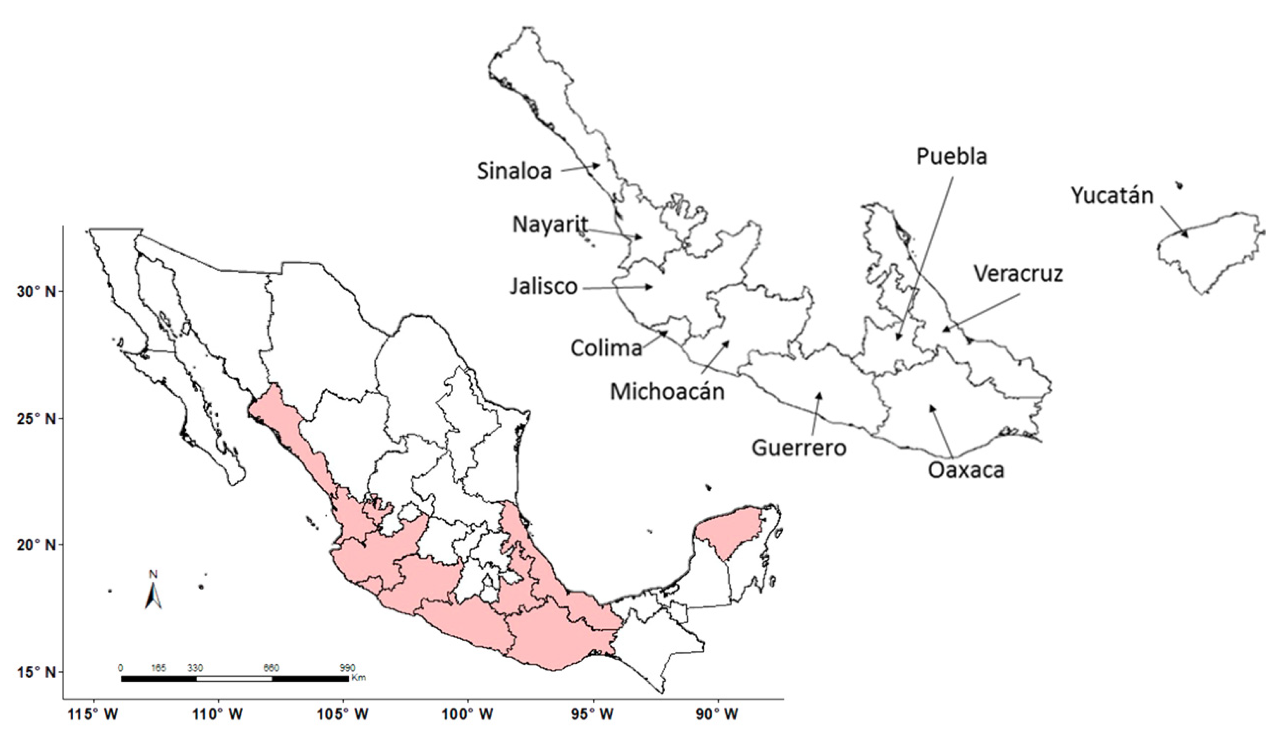
This study focuses on the wild cotton species G. aridum and the areas in Mexico where its presence has been reported, based on collections available in two databases in the country (CONABIO-SNIB [13], SINAREFI [20]) (Figure S1). The species is present mainly in the coastal states of Sinaloa, Nayarit, Jalisco, Colima, Michoacan, Guerrero, Oaxaca, Yucatan, and Veracruz (Figure 1). It is also present in the interior of Mexico, in the state of Puebla.
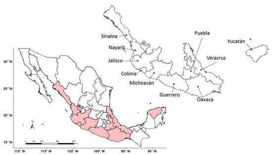
Figure 1.
Ten Mexican states with collection sites of Gossypium aridum based on 2010–2015 data of SINAREFI [20].
2.2. Plant Databases
The study used data from two Mexican databases: (1) the 2010–2015 database of the Red de Algodon del Sistema Nacional de Recursos Fitogeneticos para la Alimentación y la Agricultura (SINAREFI) [20] and (2) the database of the Comision Nacional para el Conocimiento y Uso de la Biodiversidad–Sistema Nacional de Informacion Biologica (CONABIO-SNIB) accessed in 2021 [13]. The data were analyzed to determine their quality and accuracy, following this process: First, the collection sites were projected onto geographic information systems (GIS), and the following information was obtained for each site: state, municipality, latitude, longitude, and altitude. Next, the information was compared with that reported in the passport file of each collection site to check for any disparity which would require further analysis. The data from SINAREFI and CONABIO-SNIB did not show any errors. Sites in gardens or small family farms in urban areas were eliminated.
The G. aridum data from SINAREFI [20] were partitioned as follows: 8 sites for characterization and 29 for calibration. The second database (CONABIO-SNIB [13]) contained 291 sites of G. aridum, which were used as presence data for model validation and sensitivity analysis. The database also contained information on other wild cotton species that were used to obtain the pseudo-absence sites for the analysis. In total, 266 sites were used as pseudo-absences.
2.3. Climate Database and Parameters
Mexico has a digitized cartographic database at the country level at scales from 1:1,000,000 to 1:50,000, which integrates vegetation, soil, topography and other information. In the present study, the climate vector data set (minimum and average temperature and precipitation in monthly and annual averages) with a scale of 1:1,000,000 [21] was used to generate specific climatic parameters of interest for the study, namely annual available soil water (AASW), real annual evapotranspiration (ETR, a component of AASW), and growing degree days (GDD) for flowering. These variables were chosen based on results of other studies [22,23] and consultations with Mexican wild cotton specialists. GDD is a means to predict the growth stages of the plant, considering accumulated heat [23,24]. Temperature and water stress are major factors affecting seed germination, seedling establishment, and crop success [25,26]. Extreme water shortages constrain germination and seedling establishment [26,27], while higher temperatures during vegetative/reproductive stages harm the overall progress of the crop, resulting in seed cotton yield losses [28].
2.3.1. Annual Available Soil Water
The annual available soil water (AASW) is calculated as the difference between annual precipitation and real annual evapotranspiration [29].
where:
AASW = Annual available soil water (mm yr−1)
Ppt = Mean annual rainfall (mm)
ETR = Real annual evapotranspiration (mm)
Real annual evapotranspiration is the evapotranspiration that actually occurs under the existing conditions in each case. This parameter is contrary to the potential evapotranspiration which will occur if soil moisture and plant cover were in optimal conditions. ETR was calculated using the Turc method [30,31], considering ETR as a function of long- term mean rainfall and temperature and using the following equation [31]:
where:
ETR = Real annual evapotranspiration (mm yr−1)
Ppt = Mean annual rainfall (mm)
Lc = 300 + 25t + 0.05t3
t = Mean annual temperature (°C)
2.3.2. Growing Degree Days for Flowering
Plants require a specific amount of heat units to develop from one stage of development to another. Physiological estimations considering the measurement of accumulated heat units over time have proven more accurate than the number of calendar days [24]. Growing degree days (GDD), also known as heat units (HUs) or thermal time, is an essential indicator of crop phenology, with the potential to show crop development and forecast cotton phenology [32]. It is based on the premise that the growth of plants is related to temperature, and plant development will occur only when the temperature exceeds a specific base temperature (tb) for a certain number of days [33]. Supak [34] commented that while a constant base temperature is usually used for the full growing season, the base values tend to differ in the various growth stages of the plant. In the present study, flowering growing degree days (FGDD-day °C) was used to predict potential distribution areas. Flowering is considered the prime physiological stage of the cotton plant, indicating the reproductive stage and determining the final productivity [28]. In other studies, GDDs have been calculated with the base temperature ranging from 12 °C to around 15 °C [28]. This study considered a base temperature of 18 °C for flowering [35,36].
FGDD was calculated as follows:
where:
Tm = mean daily temperature (°C)
Tt = threshold minimum temperature for flowering (18 °C for this study).
The mean daily temperature was obtained from the monthly averages by sine curve interpolation between mid-months to obtain quasi-daily values [37].
2.4. Characterization of the Sites
In ecology, knowledge of the factors influencing the distribution of organisms is essential and has many potential applications [38]. Observations on the distribution of a species provide valuable information regarding its environmental requirements [39]. In this study, characteristics that distinguish the collection sites of G. aridum in Mexico were described.
G. aridum has been reported in both coastal areas and mountainous areas of ten states of Mexico (Figure 1). Thus its distribution is wide in terms of territory and climatic conditions. In this study, we used a reduced number of sites located throughout a single state that has a wide range of climatic conditions. This modeling approach can be used when there is a small number of data available for a species of wide territorial and climatic distribution. We selected eight collection sites in the state of Sinaloa reported in the SINAREFI database. These sites were chosen because they are located throughout the state, covering different climatic conditions (temperature and precipitation), thereby making it possible to detect the various conditions in which the species could establish itself.
The selected sites were located in both coastal and mountainous areas. The predominant climates in Sinaloa, by territorial extension, are as follows: warm sub-humid (37.1%), warm semi-dry (21.3%), warm dry (18.6%), semi-warm sub-humid (11.0%), warm very dry (9.7%), and temperate sub-humid (2.3%). The regions with the highest temperatures (more than 22 °C) are in the extreme north and south of the territory, while the regions with the lowest temperatures (between 12 and 18 °C) are in the mountain ranges of the Sierra Madre Occidental. The average annual precipitation in the state is 790 mm; rains mainly occur in the summer, from July to September. Rainfall is scarce on the coasts and increases on the foothills of the Sierra Madre Occidental.
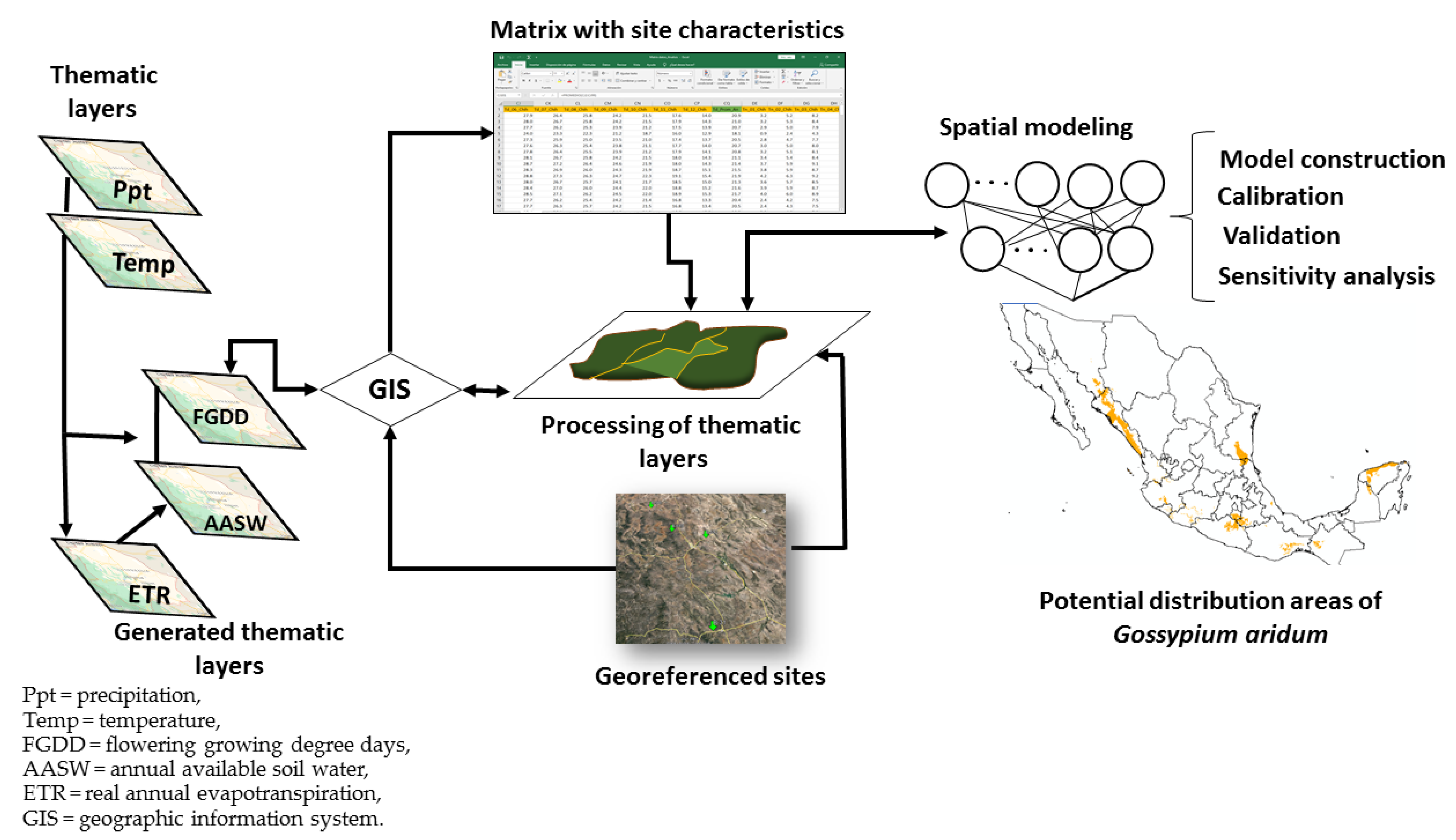
The values of the AASW and FGDD variables were obtained for each site through the use of ArcGIS software 10.3 of Esri, Inc.® (Redlands, CA, USA). This resulted in a data matrix with the climatic (temperature and precipitation) characteristics of the presence sites of the species. Figure 2 outlines the actions carried out during the characterization phase and in other phases of the study.
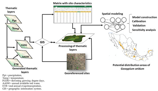
Figure 2.
Scheme of the area characterization process and modeling of the potential. distribution of the cotton species Gossypium aridum in Mexico.
2.5. Model Construction
The aim of the model-construction phase was to generate a model of the geographic distribution of the species G. aridum in Mexico based on the overlay of different thematic images with the characteristics of the collection sites of the species. The spatial processing system and the database management system of a geographic information system (GIS) made it possible to put together different types of datasets, make them compatible, and combine and analyze them [40].
The data matrix generated during the characterization process was used to derive the intervals formed by the maximum and minimum values of the AASW and FGDD variables. Prior to model construction, images with data falling within the interval defined for each variable had been generated. The model is the result of the overlay of these images using ArcGIS.
2.6. Model Calibration
Calibration is the adjustment of parameters to improve the capacity of the model to predict the dataset used for verification [41]. In this study, calibration involved the reduction of omission and commission errors. Omission errors are when the species was found, but the model predicted absence (false negatives); commission errors are when the species was not found, but the model predicted presence (false positives).
To decrease the omission errors, the values of each variable for the presence data “sensu lato” that fell outside the model were verified in order to determine the variables and the intervals to be modified. In addition, 29 sites from the SINAREFI database [20] that had not been previously used were also included during calibration. Fortunately, these 29 sites were collections reported in the states of Nayarit, Jalisco, and Colima, which was favorable for calibration in these areas where the model projected only a small potential distribution area for G. aridum.
2.7. Model Validation
Validation involved comparing the model with a set of independent observations to verify if the model was developed as expected [41,42]. For modeling based on presence records only, methods requiring both presence and absence records have been applied in other studies by sampling pseudo-absences from the study area in place of real absence data [43,44]. For this type of validation in this study, 291 collection sites of G. aridum (presence) from the CONABIO-SNIB database were used. Data of 266 sites of four other cotton species, namely, G. barberense, G. trilobum, G. gossypiodis, and G. schwendimanii, were used as pseudo-absence. These four species were selected because they did not present any association with the species G. aridum, according to the CONABIO-SNIB database.
The conversion of temperature and precipitation vector data to raster data involved changes in the form and dimension of some areas. Furthermore, during the validation, areas in the model were compared against points (presence and absence data), which means that there were areas with possible omission errors. Hence, the distances between the presence data excluded from the model and the model were measured, and the excluded sites that were located not more than 1 km outside of the model were classified as presence data “sensu lato”. To carry out the measurement, a mesh with a spacing of 1 km between centroids was generated using the Data Management Tools of the ArcGIS software. On the other hand, the sites located within the model, directly obtained with the Extraction Spatial Analysis Tool of ArcGIS, were classified as presence data “sensu stricto”. The statistics for model precision and agreement were obtained with the presence data “sensu lato” as well as “sensu stricto”.
2.8. Sensitivity Analysis
Sensitivity analysis involves the study of the variation in model output, how it can be apportioned, qualitatively and quantitatively, to different sources of variation and how the model depends upon the given input [45].
The sensitivity analysis phase was based on the jackknife (or leave-one-out) procedure [46]. The full ranges of AASW and FGDD variables of the models tested during the validation phase were first analyzed. The objective was to determine the sites and/or localities with extreme values for the two variables. The majority of the minimum values of FGDD and the maximum values of AASW were located in the collection sites in the state of Nayarit. Considering this and the ranges of the variables, four models were constructed that made it possible to determine the variation in the predictive power of the model by including or eliminating the extreme values detected in both variables.
First, a pattern model (Stone base) (Model A) was generated. It included the AASW and FGDD gradients contained in the models analyzed during the model validation process.
A second model (Model B) was generated with the same AASW values as Model A. However, in FGDD, the range of minimum values detected in the Nayarit localities was eliminated.
A third model (Model C) was generated by removing the highest range of AASW values. But the FGDD values similar to those in Model A were retained.
In the fourth model (Model D), the minimum range of FGDD was eliminated as well as the highest range of AASW. Thus, this model excluded all the Nayarit locations.
These models were tested with a total of 291 collection sites of G. aridum as presence and 266 sites of other species as pseudo-absence, all from the CONABIO-SNIB database. The “sensu strictum” and “sensu lato” sites were quantified using the methodology described in the validation phase and were used to assess model precision and agreement statistics.
2.9. Statistical Analysis
For presence-absence studies, statistics are usually derived from a 2–2 confusion matrix which indicates how often and how accurately presences and absences are predicted [41]. In order to evaluate the performance of each model, it is necessary to derive matrices of confusion that identify true positives, false positives, false negatives, and true negatives predicted by each model [42,47]. The values from the matrix of confusion are then used to calculate other performance measures, such as overall prediction success [48], sensitivity, and specificity, as well as odds ratio and Cohen’s kappa [49], both of which can better assess the ability of the models to predict presence compared to chance expectations [47,50].
In the present study, the non-parametric statistics applied in the validation and sensitivity analysis processes were the kappa index, overall accuracy, sensitivity, specificity, positive predictive power, negative predictive power, and odds ratio.
The kappa index is a measure of agreement indicating the reliability of the data obtained, which ranges from 0, signifying no agreement between observed and predicted distributions, to 1, indicating perfect agreement. Cohen’s kappa is considered a simple but effective statistical tool for the comparison and evaluation of presence-absence models [51,52].
Overall accuracy is the measurement of correct classification made by the model.
Sensitivity is the conditional probability that case X is correctly classified as true.
Specificity is the conditional probability that a case that is not X is correctly classified as false.
Positive Predictive power assesses the probability that a case is X if the algorithm classifies the case as X.
Negative Predictive power assesses the probability that a case is not X if the algorithm does not classify the case as X.
Odds Ratio is the ratio of correctly assigned cases to incorrectly assigned cases [52].
where:
a = correctly predicted presence data
b = incorrectly predicted presence data
c = incorrectly predicted absence data
d = correctly predicted absence data
n = sum of a + b + c + d
3. Results and Discussion
3.1. Characterization of the Sites
In the characterization process, an approximation of the profile of the G. aridum species was generated from the minimum and maximum values of the variables that were analyzed in the study. The characteristics were 4–76 mm year−1 AASW and 460–580 FGDD. These values present a considerable range, demonstrating the breadth of conditions in which G. aridum develops in the wild.
The ACE website [53] reports that the cotton plant under commercial cultivation requires 750 to 850° heat units calculated with a base temperature of 15.5 °C from planting to first flower. However, while the number of accumulated heat units between growth stages is assumed to be constant, it actually varies between years due to environmental factors [34]. In this study, the FGDD calculation considered a base temperature of 18 °C.
The AASW values (4 to 76 mm year−1) show that this species does not present any notable xeromorphic adaptations, but has adjusted its life cycle to rather extreme degrees and is adapted to arid environments. It has been reported as tolerant to salinity and drought [13,15,18]. Fryxell [54] mentions that G. aridum occurs in areas subjected to the wet season/dry season cycle. It has green leaves only in those months when moisture is plentiful, and it is completely leafless for about half of each year. At about the time leaves are lost, floral initiation begins, and flowering and fruiting occur during the height of the dry season.
3.2. Model Construction
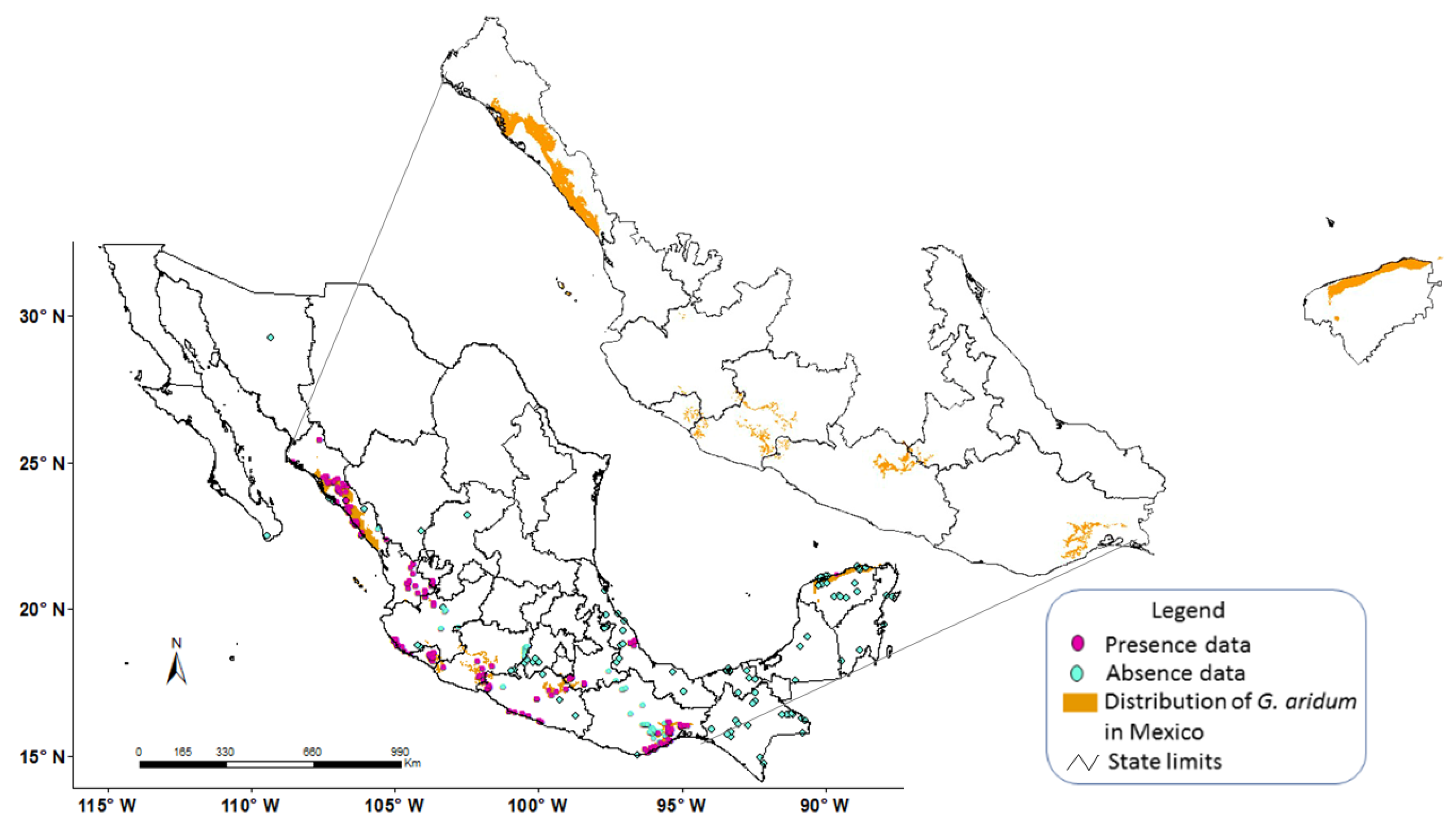
When the generated model Aridum_18 (named after the species and the base temperature) that had been constructed with the digital layers of AASW (4–76 mm year−1) and FGDD (460–580) was projected throughout Mexico (Figure 3), potential distribution areas of the species were identified in the states of Nayarit, Jalisco (border between the two states), Colima, Michoacán, Guerrero, Puebla, Oaxaca, and the northern part of Yucatán. A potential area was also detected in the four Pacific islands located off the coast of Nayarit. The largest potential areas were projected in the states of Michoacán, Guerrero, Oaxaca, and Yucatán.
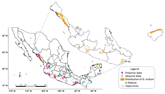
Figure 3.
Aridum_18 Model (before calibration) with presence and absence data and potential distribution of Gossypium aridum in Mexico.
From an analysis of the images that make up the model, it could be inferred that the FGDD was the primary factor in the distribution due to its lower number of pixels, leaving out a large part of the central zone of the country as well as the northeast and northwest of Mexico.
Statistical analyses of the Aridum_18 model (Figure 3) showed high values for the sensitivity test (0.70) and the negative predictive value (0.89). On the other hand, relatively low values were for overall accuracy, specificity, and positive predictive value tests, with 0.55, 0.52 and 0.24, respectively. The high value for sensitivity and low value for specificity decreased its kappa index (0.12) and odds ratio (2.45). The sensitivity and specificity values indicated extreme dimensions of the models, i.e., an excessive or else a much reduced surface. According to the information contained in the CONABIO-SNIB database, accessions of G. aridum have been collected in the states of Nayarit (central zone), Jalisco (coastal zone), and Veracruz (central zone) (Figure 3). However, the Aridum_18 model only predicted some small areas (omission error) in the border between Nayarit and Jalisco (central part) and none in Veracruz. Therefore, it can be inferred that the ranges of the variables of the Aridum_18 Model did not include the AASW and FGGD conditions in which the species G. aridum develops in these states, which apparently were very different from the areas where the species was present in the rest of the country.
3.3. Model Calibration
Five models resulted from the adjustments in the intervals of the variables of the Aridum_18 model during calibration (Table 1). The AASW variable had intervals with values of 0–210 mm year−1. CONABIO-SNIB [13] mentions that G. aridum is adapted to arid conditions and is drought tolerant [15,18]. In relation to the FGDD variable, it was observed that G. aridum also presented several intervals, with high values for the coastal areas of the states of Jalisco, Colima, and Oaxaca, and low values for the areas in the mountains of Michoacán and Guerrero (Table 1).

Table 1.
Models obtained during the calibration process to reduce omission and commission. errors in the distribution model of Gossypium aridum in Mexico.
3.4. Model Validation
Table 2 shows the results of the seven validation tests for the five models fitted with the intervals of the variables. Model 1 had the highest values in the seven tests, showing a balance between sensitivity (0.85) and specificity (0.74), which was reflected in the kappa index value (0.58). The range of variables considered in Model 1 (Table 1) extended the distribution areas of G. aridum on the coasts of Jalisco, Oaxaca, and Colima, as well as in the central part of Michoacan. However, the model did not predict areas in Nayarit and Veracruz that were covered by the variable ranges in Model 3 and Model 5 (Table 1). These two models obtained the lowest values in the specificity test (0.65), indicating that despite being able to predict distribution areas in these states, they were not selective enough for the species.

Table 2.
Results of concordance and accuracy tests.
Model 2 increased the distribution areas of the species in the coastal areas of Oaxaca and Jalisco but reduced the areas of Sinaloa, Puebla, and Guerrero. Its specificity and positive predictive power values were 0.70 and 0.66, respectively, with a kappa index of 0.53 (Table 2).
Model 4, which had the lowest values for AASW (0–77 mm year−1) but the highest for FGDD (460–860) (Table 1), and which was constructed considering the range of FGDD and AASW values of the Guerrero sites which did not fit in the intervals of other areas, reduced the distribution of the species in the areas of Sinaloa, Puebla, and part of Oaxaca. However, integrating high values of FGDD increased the distribution areas in the coastal areas of Jalisco, Colima, and Oaxaca, which was reflected in commission errors in these areas. Model 4 obtained the lowest value in the sensitivity test (0.79).
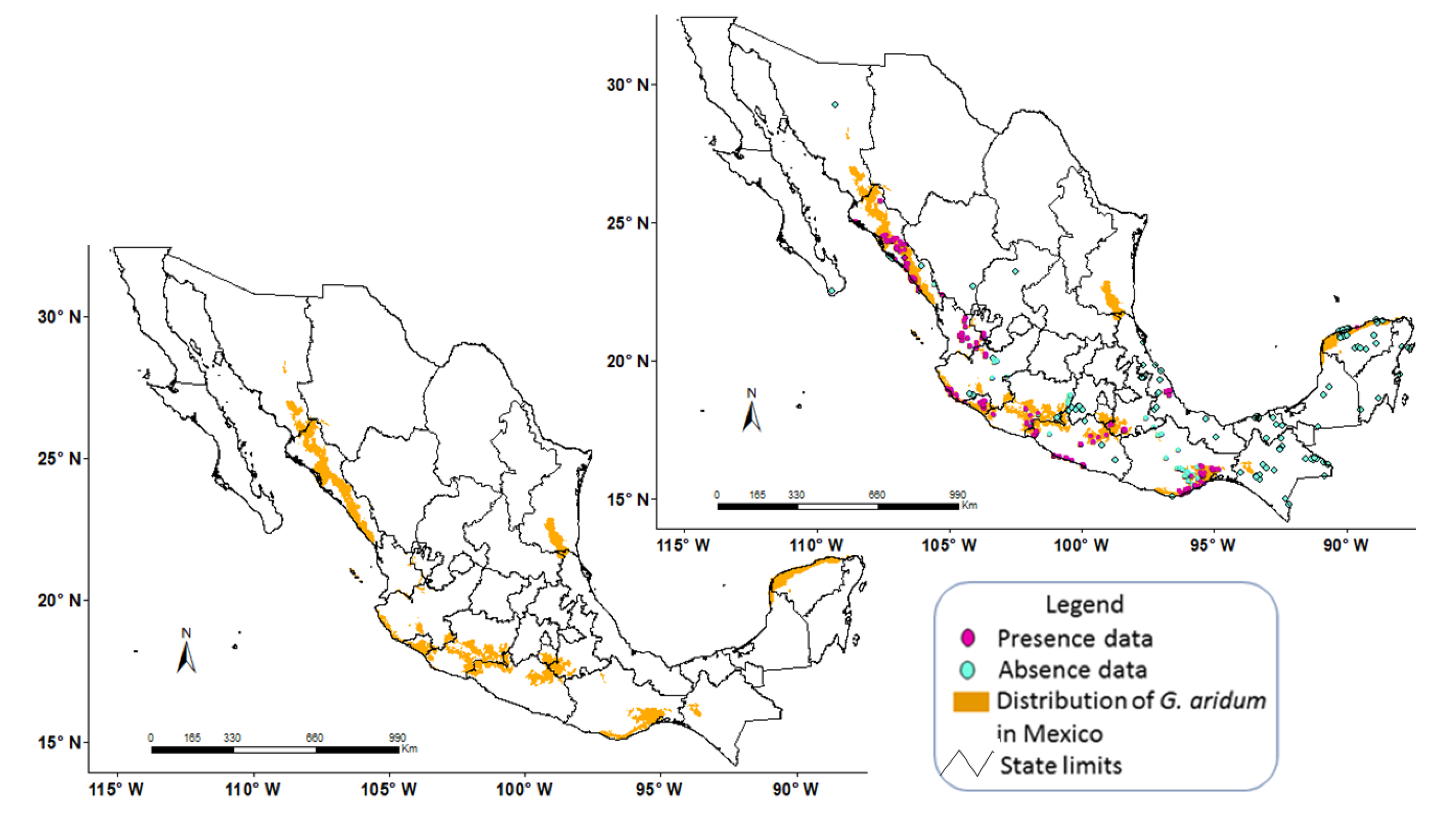
Model 1, which obtained the highest value in the kappa index and specificity test, with 0.58 and 0.74, respectively (Table 2), proved to be the most selective for the species, and best represented the distribution of G. aridum in Mexico (Figure 4).
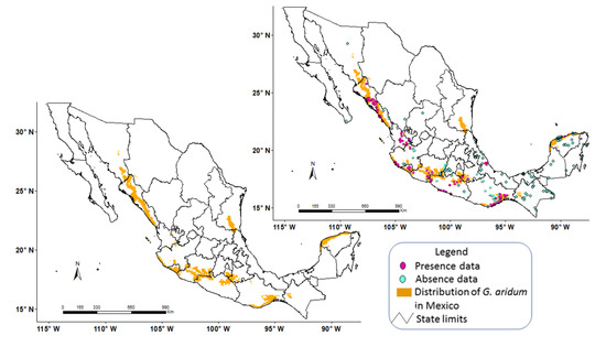
Figure 4.
Gossypium aridum Model 1 (after calibration) with presence and absence data and potential distribution of G. aridum in Mexico.
3.5. Sensitivity Analysis
To determine the climatic variable greatly influencing the distribution of the species in Mexico, four models were constructed considering the full range of intervals of the AASW and FGDD of the models tested during model validation (Table 1). In order to distinguish these four models from the previous ones, we named them using letters instead of numbers (Table 3). The results of the concordance and accuracy tests applied to these models are presented in Table 4.

Table 3.
Minimum and maximum values of variables used in the sensitivity analysis of the potential distribution of Gossypium aridum in Mexico.

Table 4.
Concordance and accuracy tests applied to the models developed in the sensitivity analysis of the potential distribution of Gossypium aridum in Mexico.
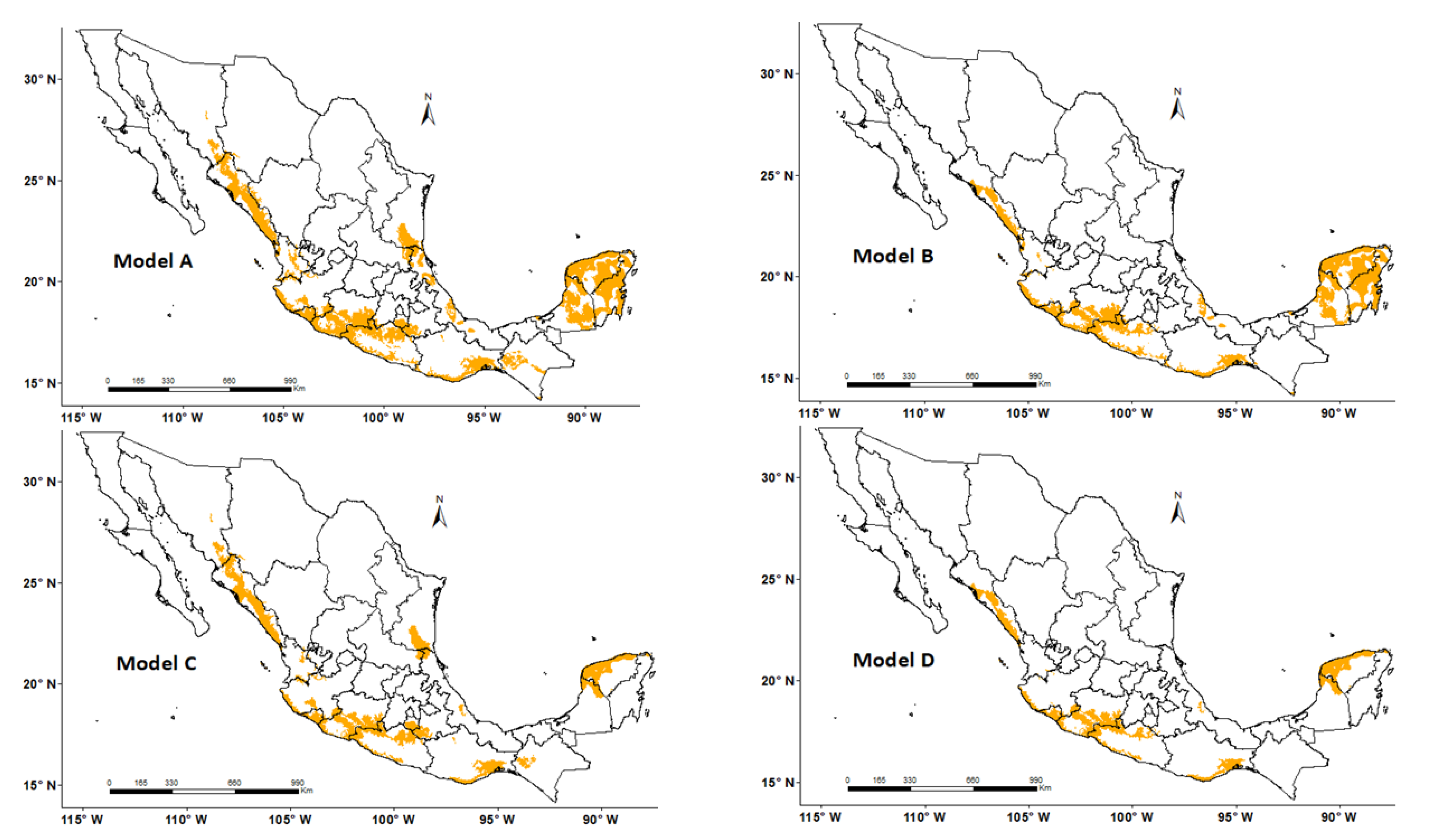
The highest values of kappa index (0.67), sensitivity (0.85), and specificity (0.82) were for Model C (Figure 5 and Table 3). The model had values of more than 0.80 in five of the non-parametric statistical tests; its kappa index value indicated a substantial level of agreement [55]. This model integrates the general range of FGDD (330–860) and AASW (4–110 mm year−1) (Table 3).
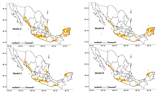
Figure 5.
Modeled potential distributions of Gossypium aridum in Mexico using four different ranges of flowering growing degree days (FGDD) and annual available soil water (AASW). Model A: 330–860 FGDD and 4–110 and 150–210 mm year−1 AASW; Model B: 460–860 FGDD and 4–110 and 150–210 mm year−1 AASW; Model C: 330–860 FGDD and 4–110 mm year−1 AASW; Model D: 460–860 FDGG and 4–110 mm year−1 AASW. Predicted areas are shaded in yellow.
Model A (pattern model) obtained similar values as Model C in three concordance and accuracy tests. A comparison of the statistical results of the two models showed that the specificity value of Model A was only 2% higher than that of Model C (0.84 vs. 0.82) but its kappa index was 3% lower than that of Model C (0.64 vs. 0.67). Models A and C differed only in the AASW variable; Model C does not contain the highest gradient (150–210 mm year−1) of this variable. Therefore, the inclusion of the two AASW gradients (Table 3) had no impact on the accuracy of the model. This is confirmed by the test values obtained by Model B, which included the two gradients of AASW (4–110 and 150–210 mm year−1) but did not include the lowest value of FGDD (i.e., 330–460). This model had the lowest values of kappa index (0.53) and specificity (0.72).
It can be concluded that FGDD is a more dominant factor than AASW for the species because it was the only variable of these two that caused changes in the distribution. According to Gertseva et al. [56] the organisms in a population can change their distribution depending on the values of the dominant factor but not in response to the values of subdominant factors.
The results of this study are similar to those of others [28,57] indicating that global temperature increases would affect cotton yield more than future changes in rainfall, thereby signaling the need to develop heat-resistant rather than drought-resistant cultivars. Reddy et al. [58] recommended breeding both heat- and cold-tolerant cultivars to cope with climate change. The use of CWRs (crop wild relatives) such as G. aridum in the development of cultivars that can stand biotic and abiotic stresses could be explored in this regard.
In order to carry out a more detailed analysis of Model A and Model C, which considered the full range of FGDD and obtained the highest values in the concordance and accuracy tests, images were generated for geographical regions covered in the present study (Figure 6 and Figure 7). Model A, by integrating all the FGDD and AASW gradients, overestimated (commission error) the hilly areas of Sinaloa and Nayarit, as well as zones in central Nayarit and coastal areas of Jalisco (Figure 6).
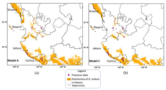
Figure 6.
Gossypium aridum potential distribution Models A (a) and C (b) with presence data of G. aridum in the states of Sinaloa, Nayarit, Jalisco and Colima in Mexico.
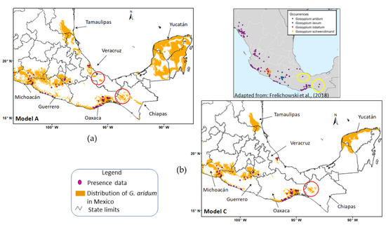
Figure 7.
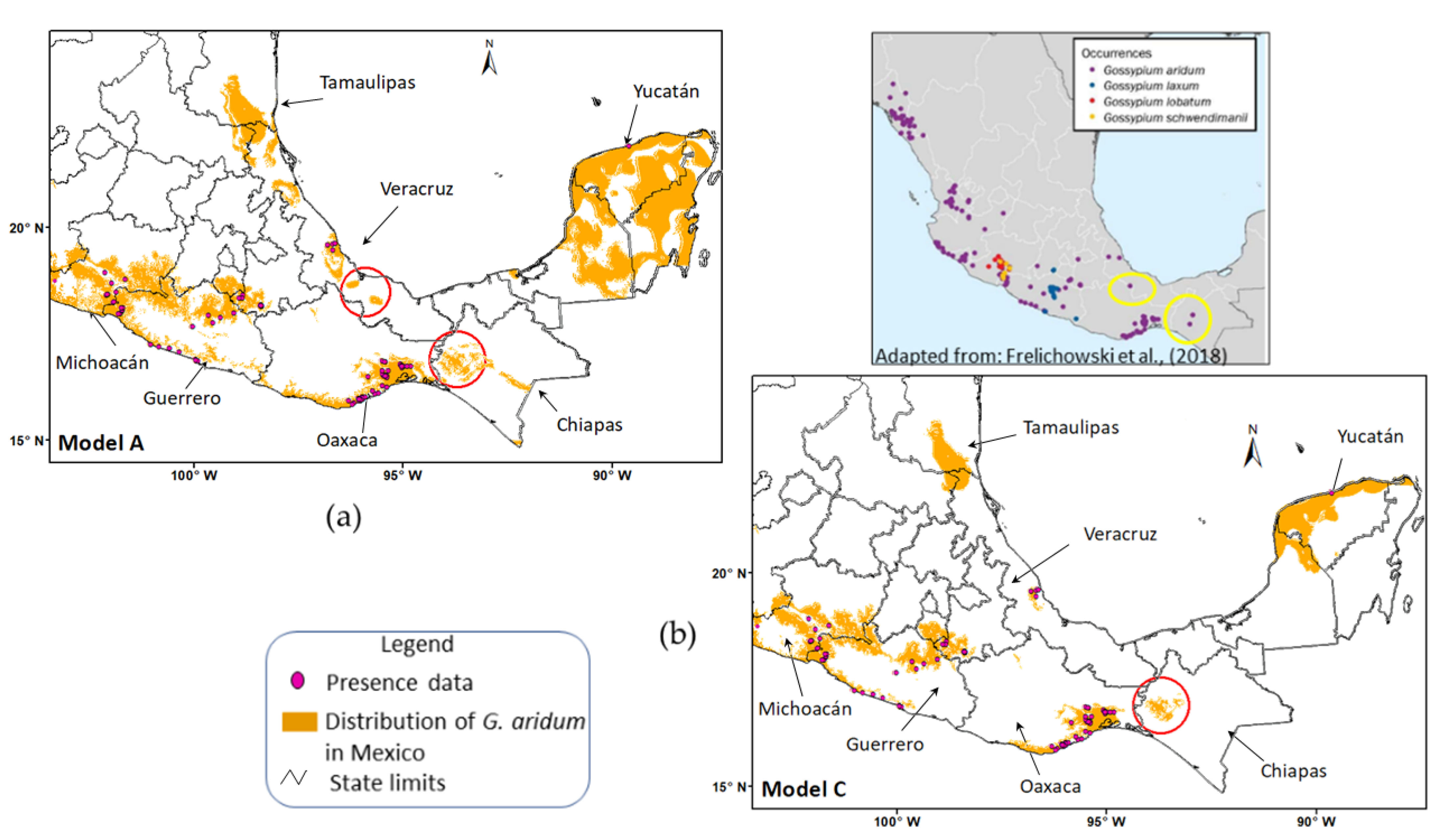
Gossypium aridum Models A (a) and C (b) showing presence data and potential distribution of G. aridum in the states of Michoacan, Guerrero, Oaxaca, Veracruz and Yucatan in Mexico. Areas encircled in red in Model A and Model C are areas overpredicted by the models. Areas encircled in yellow in the occurrence map adapted from Frelichowski et al. [19] indicate sites of occurrence of G. aridum in Veracruz and Chiapas reported in the Global Crop Wild Relatives Occurrence Database, Global Biodiversity Information Facility and the US National Cotton Germplasm Collection.
On the other hand, Model C, despite not integrating the highest values of AASW (150–210 mm year−1) and those that were detected in Nayarit, was able to predict certain areas of this state, leaving out only the area in the state’s central part. Both Model A and Model C overpredicted certain areas of distribution of the species in the vicinity of Nayarit and Jalisco. As mentioned by Raxworthy et al. [59], the regions that the model overpredicts show potential for identifying unknown distributional areas. These overpredicted areas in Nayarit and Jalisco can thus be the object of directed collection expeditions; they may also be considered as potential areas for species establishment.
For the distribution predicted by Model A and Model C in the states in the northeastern and southern regions of Mexico, Model A overpredicted some areas in the states of Tamaulipas, Veracruz, Yucatan, and Chiapas (Figure 7). On the other hand, model C overpredicted only some areas in Tamaulipas, Yucatan, and Chiapas (also Figure 7).
The results were corroborated through comparison with maps reported by Frelichowski et al. [19], Sanchez-Reyes et al. [60] and Vaca [61]. Frelichowski et al. [19] showed collection sites of G. aridum reported in the cotton database of the Global Crop Wild Relatives Occurrence Database, Global Biodiversity Information Facility, and the US National Cotton Germplasm Collection [19]. They reported some collection sites in Chiapas and Veracruz in the same areas where the models in the present study overpredicted the distribution of the species (Figure 7. red circles), thus corroborating the level of precision of Model A and Model C in predicting the potential distribution of G. aridum in Mexico. As mentioned earlier, overpredicted regions can signify unknown potential distribution areas of the species [59].
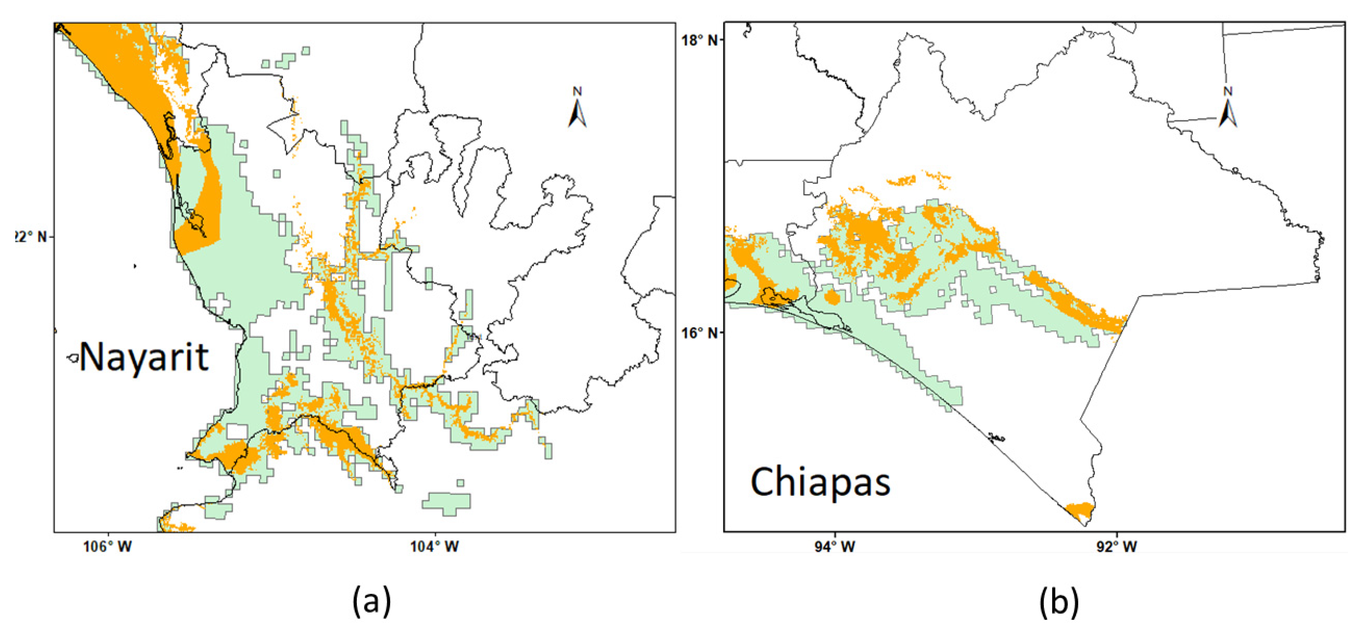
Vaca [61] modeled the potential distribution of G. aridum in Mexico using GAM (generalized additive models) and RPART (Recursive Partitioning and Regression Trees) and annual dynamics in soil moisture as a predictive variable. The comparison between distribution areas projected by Vaca vs. the present study was made by superimposing the shape files of both studies using ArcGIS. The area predicted by Vaca had larger extensions projected in the states of Nayarit, Guerrero and Oaxaca; however, no statistical tests were reported in his study. In addition, the author did not report any distribution area in Yucatan, a possible error of omission as there are records of collections made in this state contained in the CONABIO-SNIB database. On the other hand, Vaca [61] projected areas in the states of Chiapas and Veracruz similar to those in our study.
The collection sites reported by Frelichowski et al. [19] and the potential distribution determined by Vaca [61] and Sanchez-Reyes et al. [60] corroborate the areas where the distribution model constructed in the present work projects G. aridum areas, although a comparison of distributions predicted by Vaca [60] and those predicted by the present work shows a great difference in terms of area extension. An example is presented in Figure 8, where, in regions such as Nayarit and Chiapas, these differences are evident in predicted area detail. Unfortunately, as mentioned previously, Vaca [61] did not present any statistical support or additional data with which statistical and other comparisons could be made.
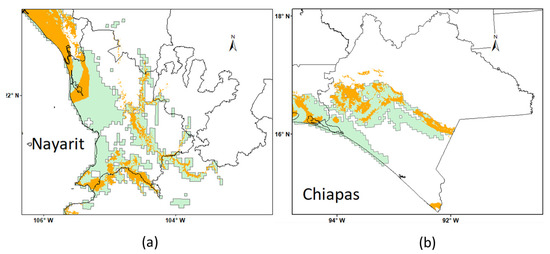
Figure 8.
Comparison of the predicted distribution of Gossypium aridum in present study (yellow area) versus the potential distribution reported by Vaca [60] (green area) in the states of Nayarit (a) and Chiapas (b), Mexico.
According to Pearson et al. [46], modeled distributions using small samples must not be interpreted as representing limits to the range of the species. Rather, they represent regions with environmental conditions similar to those in locations where the species currently have populations. The biogeographical information they yield can be useful in discovering unknown populations and species [59,62]. This is demonstrated in the distribution predicted by Models A and C in the state of Chiapas (Figure 7), which shows the presence of some areas with the environmental conditions suitable for the species. Models demonstrating significant predictive ability in jackknife tests can guide field surveys [41].
4. Conclusions
By using two environmental variables—flowering growing degree days and annual available soil water (mm year−1)—it was possible to model the observed and potential distribution of the wild species G. aridum in Mexico and identify the values of FGDD and AASW required by this species. The ranges of 330–860 FGDD and 4–110 mm year−1 AASW best described the species habitat, according to results of seven precision and accuracy statistical tests. In this study, flowering growing degree days showed greater influence on the distribution of G. aridum in Mexico.
The modeling approach developed for this study identified geographic regions in the country that present similar conditions to where the species has been observed and which are not yet registered in the cotton databases in Mexico. Some of these new locations were corroborated during comparisons with published maps generated in other studies that used information from local and international databases, thereby indicating the accuracy of the population modeling of G. aridum in the present study. Other studies, such as field surveys, are needed to further strengthen the predictive power of the generated distribution models. The modeling approach considering two basic needs for the development and survival of the wild species G. aridum, namely, the temperature requirements for its reproduction and the amount of soil water during its annual development cycle, may be applied in the modeling of other wild cotton species.
The information generated in this study can be used to guide collection expeditions for G. aridum species and to study climatic impact on the distribution of the species. It can serve as input in studies and programs designed to characterize, conserve, and sustain the diversity of genetic resources in Mexico.
Supplementary Materials
The following supporting information can be downloaded at: https://www.mdpi.com/article/10.3390/su14116383/s1. Figure S1. Collection sites of Gossypium aridum from CONABIO-SNIB and SINAREFI databases used in modeling the distribution of G. aridum in Mexico using flowering growing degree days and annual available soil water.
Author Contributions
Conceptualization, methodology and formal analysis, A.D.B.-G.; review of analysis and results, A.M.-C., M.H.R.-M., J.R.K. and M.N.M.; writing—original draft preparation, A.D.B.-G.; writing—review and editing, all authors. All authors have read and agreed to the published version of the manuscript.
Funding
This research received no external funding.
Institutional Review Board Statement
Not applicable.
Informed Consent Statement
Not applicable.
Data Availability Statement
Publicly available CONABIO datasets were analyzed in this study. The data can be found here: https://enciclovida.mx/especies/139343-gossypium (accessed on 17 September 2021). The SINAREFI datasets used in this study are not publicly available.
Acknowledgments
The authors are grateful to the Cotton Network-SINAREFI/SNICS (2010–2015), particularly Rosario Tovar-Gomez and Claudia Perez-Mendoza, for G. aridum data used in this study and to CONABIO-SNIB for making available data on G. aridum and other Gossypium species to support scientific research in Mexico. They are also grateful to Eng. Jose Luis Ramos-Gonzalez for extending technical support during each stage of the research and to Elvira Tabobo-Aranda for editing the manuscript. They extend their sincere thanks to the anonymous reviewers for their encouraging and helpful comments.
Conflicts of Interest
The authors declare no conflict of interest.
References
- Contreras-Toledo, A.R.; Cortés-Cruz, M.A.; Costich, D.; de Lourdes Rico-Arce, M.; Brehm, J.M.; Maxted, N. A crop wild relative inventory for Mexico. Crop Sci. 2018, 58, 1292–1305. [Google Scholar] [CrossRef]
- Goettsch, B.; Urquiza-Haas, T.; Koleff, P.; Acevedo Gasman, F.; Aguilar-Meléndez, A.; Alavez, V.; Alejandre-Iturbide, G.; Aragon Cuevas, F.; Azurdia Pérez, C.; Carr, J.A.; et al. Extinction risk of Mesoamerican crop wild relatives. Plants People Planet 2021, 3, 775–795. [Google Scholar] [CrossRef]
- Hossain, A.; Maitra, S.; Pramanick, B.; Bhutia, K.L.; Ahmad, Z.; Moulik, D.; Syed, M.A.; Shankar, T.; Adeel, M.; Hassan, M.M.; et al. Wild relatives of plants as sources for the development of abiotic stress tolerance in plants. In Plant Perspectives to Global Climate Changes Developing Climate-Resillient Plants, 1st ed.; Aftab, T., Roychoudhury, A., Eds.; Elsevier: Amsterdam, The Netherlands, 2022; pp. 471–518. [Google Scholar]
- EL Sabagh, A.; Hossain, A.; Islam, M.; Barutcular, C.; Ratnasekera, D.; Gormus, O.; Amanet, K.; Mubeen, M.; Nasim, W.; Fahad, S.; et al. Drought and heat stress in cotton (Gossypium hirsutum L.): Consequences and their possible mitigation strategies. In Agronomic Crops; Springer: Singapore, 2020; pp. 613–634. [Google Scholar] [CrossRef]
- Gechev, T.; Petrov, V. Reactive oxygen species and abiotic stress in plants. Int. J. Mol. Sci. 2020, 21, 7433. [Google Scholar] [CrossRef] [PubMed]
- Majeed, S.; Chaudhary, M.T.; Hulse-Kemp, A.M.; Azhar, M.T. Introduction: Crop Wild Relatives in Plant Breeding. In Wild Germplasm for Genetic Improvement in Crop Plants; Azhar, M.T., Wani, S.H., Eds.; Elsevier Inc.: Amsterdam, The Netherlands, 2021; pp. 1–18. [Google Scholar]
- Burgeff, C.; Huerta, E.; Acevedo, F.; Sarukhán, J. How much can GMO and non-GMO cultivars coexist in a megadiverse country? AgBioForum 2014, 17, 90–101. [Google Scholar]
- Rocha-Munive, M.G.; Soberón, M.; Castañeda, S.; Niaves, E.; Scheinvar, E.; Eguiarte, L.E.; Mota-Sánchez, D.; Rosales-Robles, E.; Nava-Camberos, U.; Martínez-Carrillo, J.L.; et al. Evaluation of the impact of genetically modified cotton after 20 years of cultivation in Mexico. Front. Bioeng. Biotechnol. 2018, 6, 82. [Google Scholar] [CrossRef]
- Wendel, J.F.; Grover, C.E. Taxonomy and evolution of the cotton genus, Gossypium. Cotton 2015, 57, 25–44. [Google Scholar]
- Perez-Mendoza, C.; Tovar-Gomez, M.R.; Baez-Gonzalez, A.D.; Flores-Zarate, M. Recolección de germoplasma del género Gossypium en el estado de Guerrero. In Foro de Estudios Sobre Guerrero; COCYTIEG (Consejo de Ciencia y Tecnologia en Innovacion del Estado de Guerrero): Iguala, Mexico, 2016; pp. 1043–1047. [Google Scholar]
- Ulloa, M.; Stewart, J.M.; Acosta, N.S. Cotton genetic resources in the western states of Mexico: In situ conservation status and germplasm collection for ex situ preservation. Genet. Resour. Crop Evol. 2006, 5, 653–668. [Google Scholar] [CrossRef]
- Álvarez, I.; Wendel, J.F. Cryptic interspecific introgression and genetic differentiation within Gossypium aridum (Malvaceae) and its relatives. Evolution 2006, 60, 505–517. [Google Scholar] [CrossRef][Green Version]
- CONABIO-SNIB. Comisión Nacional Para el Conocimiento y Uso de la Biodiversidad-Sistema Nacional de Información Sobre Biodiversidad. Gossypium. Available online: https://enciclovida.mx/especies/139343-gossypium (accessed on 17 September 2021).
- Zeng, L.; Stetina, S.R.; Erpelding, J.E.; Bechere, E.; Turley, R.B.; Scheffler, J. History and current research in the USDA-ARS cotton breeding program at Stoneville, MS. J. Cotton Sci. 2018, 22, 24–35. [Google Scholar]
- Shim, J.; Mangat, P.K.; Angeles-Shim, R.B. Natural variation in wild Gossypium species as a tool to broaden the genetic base of cultivated cotton. J. Plant Sci. Curr. Res 2018, 2. [Google Scholar] [CrossRef]
- Guo, Q.; Zhao, L.; Fan, X.; Xu, P.; Xu, Z.; Zhang, X.; Meng, S.; Shen, X. Transcription factor GarWRKY5 is involved in salt stress response in diploid cotton species (Gossypium aridum L.). Int. J. Mol. Sci. 2019, 20, 5244. [Google Scholar] [CrossRef] [PubMed]
- Hu, G.; Grover, C.E.; Yuan, D.; Dong, Y.; Miller, E.; Conover, J.L.; Wendel, J.F. Evolution and Diversity of the Cotton Genome. In Cotton Precision Breeding, 1st ed.; Rahman, M., Zafar, Y., Zhang, T., Eds.; Springer: Cham, Switzerland, 2021; pp. 25–78. [Google Scholar]
- Saleem, H.; Tanees, C.M.; Shakeel, A.; Hussain, W.S.; Du, X.; Tehseen, A.M. Wild Cotton Genepool: An Unopened Treasure. In Wild Germplasm for Genetic Improvement in Crop Plants, 1st ed.; Azhar, M.T., Wani, S.H., Eds.; Elsevier Inc.: Amsterdam, The Netherlands, 2021; pp. 19–53. [Google Scholar]
- Frelichowski, J.; Jenderek, M.M.; Greene, S.; Hinze, L.L.; Love, J. Conservation of Crop Wild Relatives of Cotton (Gossypium hirsutum L.) Originating from the USA and Mexico. In Proceedings of the ASA, CSSA, and CSA International Annual Meeting, Baltimore, MD, USA, 4 November 2018. [Google Scholar]
- SINAREFI (Sistema Nacional de Recursos Fitogeneticos para la Alimentación y la Agricultura). Red de Algodón: Datos de Pasaporte de Accesiones de Algodon (2010–2015) para los Recursos Fitogenéticos para la Alimentación y la Agricultura (RFAA). D.F. México, 2015 SAGARPA/SNICS/SINAREFI.
- INEGI. Instituto Nacional de Informacion Estadistica y Geografía. Climatología. 2007. Available online: https://www.inegi.org.mx/temas/climatologia/ (accessed on 29 August 2021).
- Sharma, A.; Deepa, R.; Sankar, S.; Pryor, M.; Stewart, B.; Johnson, E.; Anandhi, A. Use of growing degree indicator for developing adaptive responses: A case study of cotton in Florida. Ecol. Indic. 2021, 124, 107383. [Google Scholar] [CrossRef]
- Fraisse, C.W.; Paula-Moraes, S.V. Degree Days: Heating, Cooling, and Growing. Agricultural and Biological Engineering Department, Florida Cooperative Extension Service, Institute of Food and Agricultural Sciences, University of Florida. Available online: http://edis.ifas.ufl.edu (accessed on 3 September 2021).
- Gudadhe, N.N.; Kumar, N.; Pisal, R.R.; Mote, B.M.; Dhonde, M.B. Evaluation of agrometeorological indices in relation to crop phenology of cotton (Gossipium spp.) and chickpea (Cicer aritinum L.) at Rahuri region of Maharashtra. Trends Biosci. 2013, 6, 246–250. [Google Scholar]
- Casenave, E.C.; Toselli, M.E. Hydropriming as a pre-treatment for cotton germination under thermal and water stress conditions. Seed Sci. Technol. 2007, 35, 88–98. [Google Scholar] [CrossRef]
- Maeda, A.B.; Wells, L.W.; Sheehan, M.A.; Dever, J.K. Stories from the Greenhouse—A Brief on Cotton Seed Germination. Plants 2021, 10, 2807. [Google Scholar] [CrossRef] [PubMed]
- Harrison, P.A. Climate Change Impacts on Agriculture in Europe: Spatial Modelling of Winter Wheat. Ph.D. Thesis, University of Oxford, Oxford, UK, 1999. [Google Scholar]
- Mudassir, M.A.; Rasul, F.; Khaliq, T.; Yaseen, M. Conformance of sowing dates for maximizing heat use efficiency and seed cotton yield in arid to semi-arid cotton zone of Pakistan. Environ. Sci. Pollut. Res. 2021, 29, 11359–11373. [Google Scholar] [CrossRef]
- Pearson, R.G.; Dawson, T.P.; Berry, P.M.; Harrison, P.A. SPECIES: A Spatial Evaluation of Climate Impact on the Envelope of Species. Ecol. Model. 2002, 154, 289–300. [Google Scholar] [CrossRef]
- Andréassian, V.; Sari, T. Technical Note: On the puzzling similarity of two water balance formulas–Turc–Mezentsev vs. Tixeront–Fu. Hydrol. Earth Syst. Sci. 2019, 23, 2339–2350. [Google Scholar] [CrossRef]
- Sanchez San Roman, F.J. Evapotranspiracion.Depto. Geologia Universidad de Salamanca. Available online: https://hidrologia.usal.es/ (accessed on 22 November 2021).
- Reddy, K.R.; Hodges, H.F.; McKinion, J.M.; Wall, G.W. Temperature effects on Pima cotton growth and development. Agron. J. 1992, 84, 237–243. [Google Scholar] [CrossRef]
- Fraisse, C.W.; Bellow, J.; Brown, C. Degree Days: Heating, Cooling, and Growing; IFAS Extension; ABE 381; 1-7EDIS; University of Florida: Gainesville, FL, USA, 2007. [Google Scholar]
- Supak, J.R. Understanding and Using Heat Units in Cotton Production Systems. In Summary of Proceedings-Western Cotton Producers Conference (USA). Available online: http://cotton.tamu.edu/General%20Production/arch-understandingandusingheat.pdf (accessed on 12 December 2021).
- Tcach, N.; Paytas, M. Incidencia de altas temperaturas durante el reproductivo sobre el rendimiento de algodón (Gossypium hirsutum) cultivado en diferentes distanciamientos entre surcos. RIA. Rev. Investig. Agropecu. 2020, 46, 56–65. [Google Scholar]
- Reddy, K.R.; Kakanl, V.G.; Zhao, D.; Kotl, S.; Gao, W. Interactive effects of ultraviolet-B radiation and temperature on cotton physiology, growth, development and hyperspectral reflectance. Photochem. Photobiol. 2004, 79, 416–427. [Google Scholar] [CrossRef] [PubMed]
- Harrison, P.A.; Porter, J.R.; Downing, T.E. Scaling-up the AFRCWHEAT2 model to assess phenological development for wheat in Europe. Agric. For. Meteorol. 2000, 101, 167–186. [Google Scholar] [CrossRef]
- Caldow, R.W.G.; Racey, P.A. Introduction: Largescale processes in ecology and hydrology. J. Appl. Ecol. 2000, 37, 6–12. [Google Scholar] [CrossRef]
- Pearson, R.G.; Dawson, T.P. Predicting the impacts of climate change on the distribution of species: Are bioclimate envelope models useful? Glob. Ecol. Biogeogr. 2003, 12, 361–371. [Google Scholar] [CrossRef]
- Guarino, L.; Jarvis, A.; Hijmans, R.J.; Maxted, N. Geographic Information Systems (GIS) and the Conservation and Use of Plant Genetic Resources. In Managing Plant Genetic Resources; Engels, J.M.M., Rao, V.R., Brown, A.H.D., Jackson, M.T., Eds.; IPGRI: Rome, Italy, 2002; pp. 387–404. [Google Scholar]
- Richardson, J.; Berish, C. Data and information issues in modeling for resource management decision making: Communication is the key. In Ecological Modeling for Resource Management, 1st ed.; Dale, V.H., Ed.; Springer: New York, NY, USA, 2003; pp. 167–179. [Google Scholar]
- Peterson, A.T.; Benz, B.W.; Papes, M. Highly pathogenic H5N1 avian influenza: Entry pathways into North America via bird migration. PLoS ONE 2007, 2, e261. [Google Scholar] [CrossRef] [PubMed]
- Ferrier, S.; Watson, G.; Pearce, J.; Drielsma, M. Extended statistical approaches to modelling spatial pattern in biodiversity in northeast New South Wales. I. Species-level modelling. Biodivers. Conserv. 2002, 11, 2275–2307. [Google Scholar] [CrossRef]
- Engler, R.; Guisan, A.; Rechsteiner, L. An improved approach for predicting the distribution of rare and endangered species from occurrence and pseudo-absence data. J. Appl. Ecol. 2004, 41, 263–274. [Google Scholar] [CrossRef]
- Saltelli, A. What is sensitivity analysis? In Sensitivity Analysis, 1st ed.; Saltelli, A., Chan, K., Scott, E.M., Eds.; John Wiley and Sons: West Sussex, UK, 2005; pp. 3–14. [Google Scholar]
- Pearson, R.G.; Raxworthy, C.J.; Nakamura, M.; Peterson, T.A. Predicting species distributions from small numbers of occurrence records: A test case using cryptic geckos in Madagascar. J. Biogeogr. 2007, 34, 102–117. [Google Scholar] [CrossRef]
- Fielding, A.H.; Bell, J.F. A review of methods for the assessment of prediction errors in conservation presence/absence models. Environ. Conserv. 1997, 24, 38–49. [Google Scholar] [CrossRef]
- Buckland, S.T.; Elston, D.A. Empirical models for the spatial distribution of wildlife. J. Appl. Ecol. 1993, 30, 478–495. [Google Scholar] [CrossRef]
- Fielding, A. How should accuracy be measured? In Machine Learning Methods for Ecological Applications; Springer: Boston, MA, USA, 1999; pp. 209–223. [Google Scholar]
- Forbes, A.D. Classification-algorithm evaluation: Five performance measures based on confusion matrices. J. Clin. Monit. 1995, 11, 189–206. [Google Scholar] [CrossRef] [PubMed]
- Sim, J.; Wright, C.C. The Kappa statistic in reliability studies: Use, interpretation, and sample size requirements. Phys. Ther. 2005, 85, 257–268. [Google Scholar] [CrossRef] [PubMed]
- Manel, S.; Williams, H.C.; Ormerod, S.J. Evaluating presence–absence models in ecology: The need to account for prevalence. J. Appl. Ecol. 2001, 38, 921–931. [Google Scholar] [CrossRef]
- Advancing Cotton Education. Growth and Development of a Cotton Plant. National Cotton Council of America. Available online: https://www.cotton.org/tech/ace/growth-and-development.cfm (accessed on 18 February 2022).
- Fryxell, P.A. The Natural History of the Cotton Tribe (Malvaceae, Tribe Gossypieae); Texas A & M University Press: Collage Station, TX, USA, 1979; p. 264. [Google Scholar]
- Landis, J.R.; Koch, G.G. The measurement of observer agreement for categorical data. Biometrics 1977, 33, 159–174. [Google Scholar] [CrossRef]
- Gertseva, V.; Gertsev, V.; Ponomarev, N.Y. Integrative model of a population distribution in a habitat. Ecol. Model. 2005, 193, 575–588. [Google Scholar] [CrossRef]
- Diarra, A.; Barbier, B.; Zongo, B.; Yacouba, H. Impact of climate change on cotton production in Burkina Faso. Afr. J. Agric. Res. 2017, 12, 494–501. [Google Scholar]
- Reddy, K.R.; Doma, P.R.; Mearns, L.O.; Boone, M.Y.L.; Hodges, H.F.; Richardson, A.G.; Kakani, V.G. Simulating the impacts of climate change on cotton production in the Mississippi Delta. Clim. Res. 2002, 22, 271–281. [Google Scholar] [CrossRef]
- Raxworthy, C.J. Introduction to the reptiles. In The Natural History of Madagascar; Goodman, S.M., Benstead, J.P., Eds.; University of Chicago Press: Chicago, IL, USA, 2003; pp. 934–949. [Google Scholar]
- Sánchez-Reyes, U.J.; Jones, R.W.; Raszick, T.J.; Ruiz-Arce, R.; Sword, G.A. Potential Distribution of Wild Host Plants of the Boll Weevil (Anthonomus grandis) in the United States and Mexico. Insects 2022, 30, 337. [Google Scholar] [CrossRef]
- Vaca, R.A. ‘Gossypium aridum. Distribución Potencial’, Escala: 1:5,000,000. Comisión Nacional para el Conocimiento y Uso de la Biodiversidad (CONABIO). 2020. Available online: http://www.conabio.gob.mx/informacion/gis/ (accessed on 2 March 2022).
- Bourg, N.A.; McShea, W.J.; Gill, D.E. Putting a CART before the search: Successful habitat prediction for a rare forest herb. Ecology 2005, 86, 2793–2804. [Google Scholar] [CrossRef]
Publisher’s Note: MDPI stays neutral with regard to jurisdictional claims in published maps and institutional affiliations. |
© 2022 by the authors. Licensee MDPI, Basel, Switzerland. This article is an open access article distributed under the terms and conditions of the Creative Commons Attribution (CC BY) license (https://creativecommons.org/licenses/by/4.0/).

