3.1. Case Studies for the Comparative Study
This paper proposes a calculus for the safety factor and the slip centre for three slopes with particular geometry (
Figure 5) and four types of homogeneous soils with specific properties (
Table 1) using, on the one hand, various limit equilibrium methods and the upper-bound limit method and, on the other hand, numerical calculations using FEM software. The selected cohesive soils provide varied strength characteristics ranging from almost non-plastic clayey sands to cohesive clays. The cohesion parameter for the cohesionless sand is considered to be as small as near zero to avoid numerical errors [
16]. In all cases, there is no external load other than the gravitational force, i.e., body force.
Motivation for choosing the four types of soils: The four types of soils are clayey silt, sandy-clayey silt, sandy-silty clay, and clay, as given in
Table 2. These types of soils are considered to model different types of soil shear strengths.
Table 2 summarises the geotechnical parameters of various soil types. The slip surface of slopes for homogeneous soils can approach a circular cylinder.
Motivation for choosing the three slope angles (gradients): To reveal that, when Varying the slope angle gradually and keeping the height of the slope and the soil parameters constant, the factor of safety increases as the slope angle decreases. The decrease in slope increases the factor of safety almost linearly. There is a strong and opposite relation between slope angle and factor of safety for the four types of soils considered.
Motivation for choosing the two heights (8 m and 3 m, respectively): Results presented in the paper show that the FoS (stability, implicitly) is not independent of the slope height, even in the case of homogeneous slopes. The factor of safety increases as the slope height decreases, as the pair of
Table 3,
Table 4,
Table 5,
Table 6,
Table 7 and
Table 8 show for the same type of soil and gradient. Results are similar for all the four types of soils investigated and using any method. This indicates a strong relationship between the slope height and the factor of safety.
Additionally, at a lower height, i.e., 3 m height, the failure mode in clays (S4) tends to be base slide for all three gradients, while at 8 m height, the failure mode tends to be toe slide. On sandy soils, the failure mode tends to be toe slide for either 3 m height or 8 m.
The reason why the study presents the stability results at 3 m height derives from the paper carried out by [
41], which indicates a lower rate of decrease in the factor of safety for slopes higher than 3 m. For slope heights less than 3 m, the factor of safety increases at a higher rate.
Slope height and slope angle can be optimized to maximize the slope factor of safety. The above tables show that the influence of decreasing slope height and angle simultaneously can also be studied.
For the limit equilibrium method (LEM), the Slide2 Rocscience Program performed the analysis, while the PLAXIS software performed the FEM analysis.
The Slide2 Rocscience Program simplifies the process of finding the safety factor and the critical slip surface on the strength of limit equilibrium methods. The software enables the study of the uncertainties regarding the slope geometry and properties of various soils, the potential failure surfaces, and the use of accurate static methods. It allows for narrowing the range of acceptable solutions and assesses the errors involved in slice methods [
8]. The LE methods used in this paper using the Slide2 Rocscience Program are the Fellenius/Petterson method, Bishop method, Janbu method, Morgenstern–Price method, and Spencer method, considering circular slip surfaces. The geometric model was nested into the Slide2 Rocscience Program software, assigning the soil properties for the specified interface [
42,
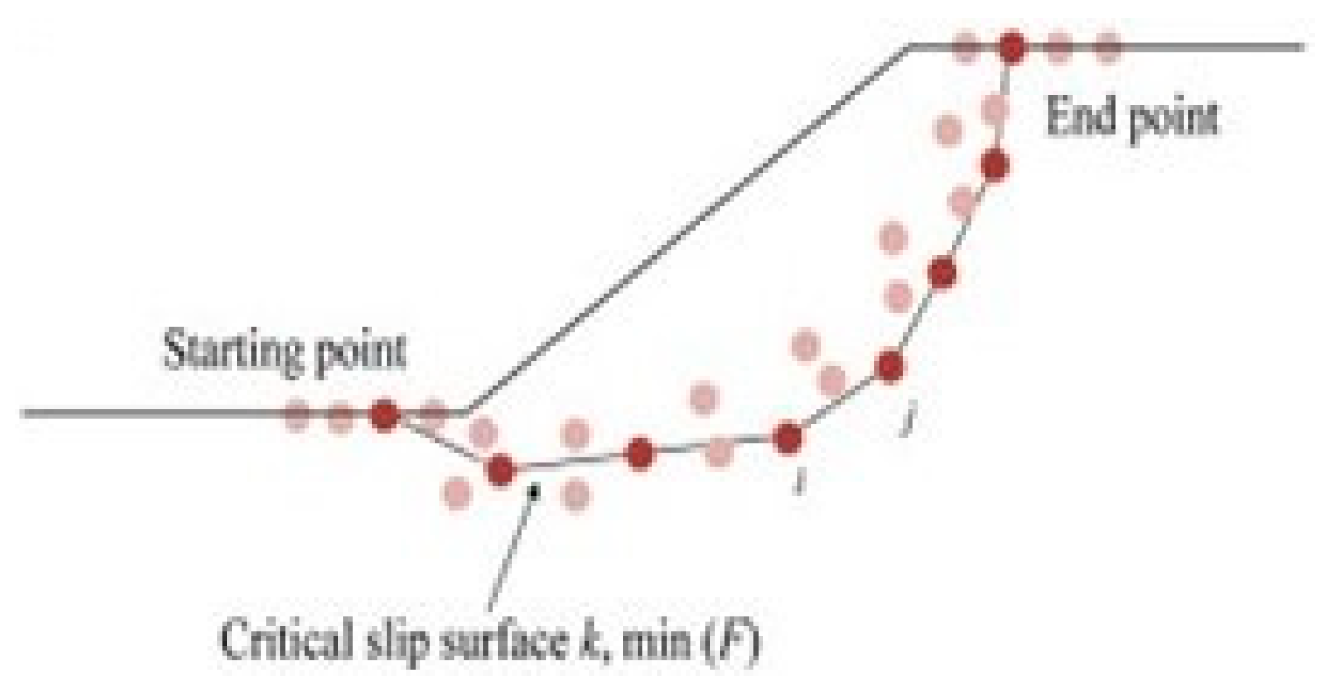
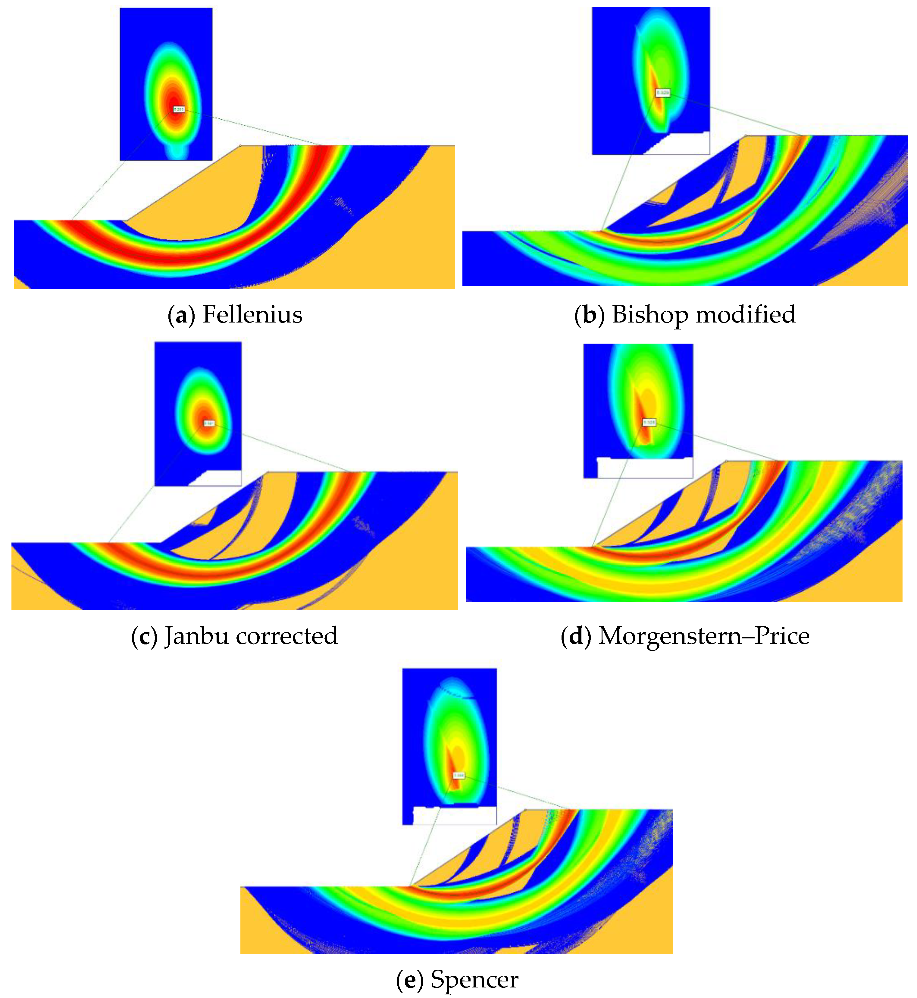
43]. In the analysis stage, a circular slip surface was in use. The limit equilibrium method of slices required iterative techniques to solve the nonlinear factor of safety equations and find the coordinates of the slip surface. In Slide2 Rocscience Program, the Grid Search Method was used for locating the Global Minimum safety factor for circular slip surfaces (
Figure 6a–e). The slip centre grid specifies the number of grid intervals in the X (80) and Y (100) directions, creating a regular grid of slip centres. Each centre in the slip centre grid represents the centre of rotation of a series of slip circles. Slide2 uses Slope Limits and Radius Increment to generate the circle’s radii at each point.
The numerical analysis used PLAXIS (2D), which is a FEM-based software. The slope divides into small elements, and a stress–strain relationship defines each case. The mesh refinement and the number of elements strongly affect the computed FoS.
The selection of the numerical model imposes large enough horizontal and vertical dimensions to not impact the results of the slope stability analysis. In the example illustrated in
Figure 7, the lateral dimensions are large, and the model maintains a similar principle regarding the depth to ensure that there is no boundary perturbation. The study considers 50 × 30 m dimensions for the model, foreseeing a slight decrease in the FoS.
All cases analysed operate with plane strains and 15-node triangular elements.
To limit the number of elements, although four polygons were constructed, only the central one had a particularly dense mesh around the slip surface (
Figure 8), ten times thicker than the other three polygons, which had moderately dense meshes. The purpose of using a fine mesh is to achieve good accuracy concerning the picked-up points according to the procedure specified in
Section 2.3.
A very dense mesh around the sloping area is an important matter. The finer the mesh, the closer the results will be to each other. However, if the “classical” mesh is maintained, FoS will not decrease dramatically. The analyses used the Mohr–Coulomb failure criterion and a perfect plastic flow with no plastic dilatancy.
3.2. Results
In most of the cases examined, the predicted failure surface passes through the toe of the slope and does not extend below this point. However, in the cases of the 1:1.5, H = 3 m, S4 slope and 1:1, H = 8 m, S1 slope, a base failure occurs, i.e., the failure surface passes below the toe.
The mesh refinement and the number of picked-up elements strongly affect the computed FoS. Furthermore, the adaptive mesh refinement influences the error margin between the upper and lower bounds.
For the cases where the safety factor is greater than 1, the slope yields through the phi-c reduction procedure. In this case, there is no difference between the diagram for total deformation (Phase 1) and that for incremental deformation (Initial Phase) (
Figure 9,
Figure 10,
Figure 11 and
Figure 12a–h).
If the stability factor is less than 1.00 (Slope 1:1, H = 8.00 m, S1; Slope 2:1, H = 8.00 m, S1; Slope 2:1, H = 8.00 m, S2), the slope yields from gravitational loading (Initial Phase).
Figure 13 shows the plastic points for the Slope 1:1, H = 8.00 m, S1, and
Figure 14 shows the result for the total deformation, a representation that cannot be useful for determining the slip surface.
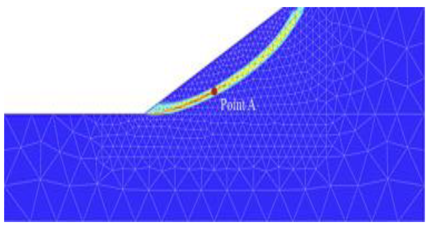
In these cases, the problem reduces to extracting from the diagram of incremental deformations that follow the slip surface (yielding surface) those points on the band of “0” (
Figure 15).
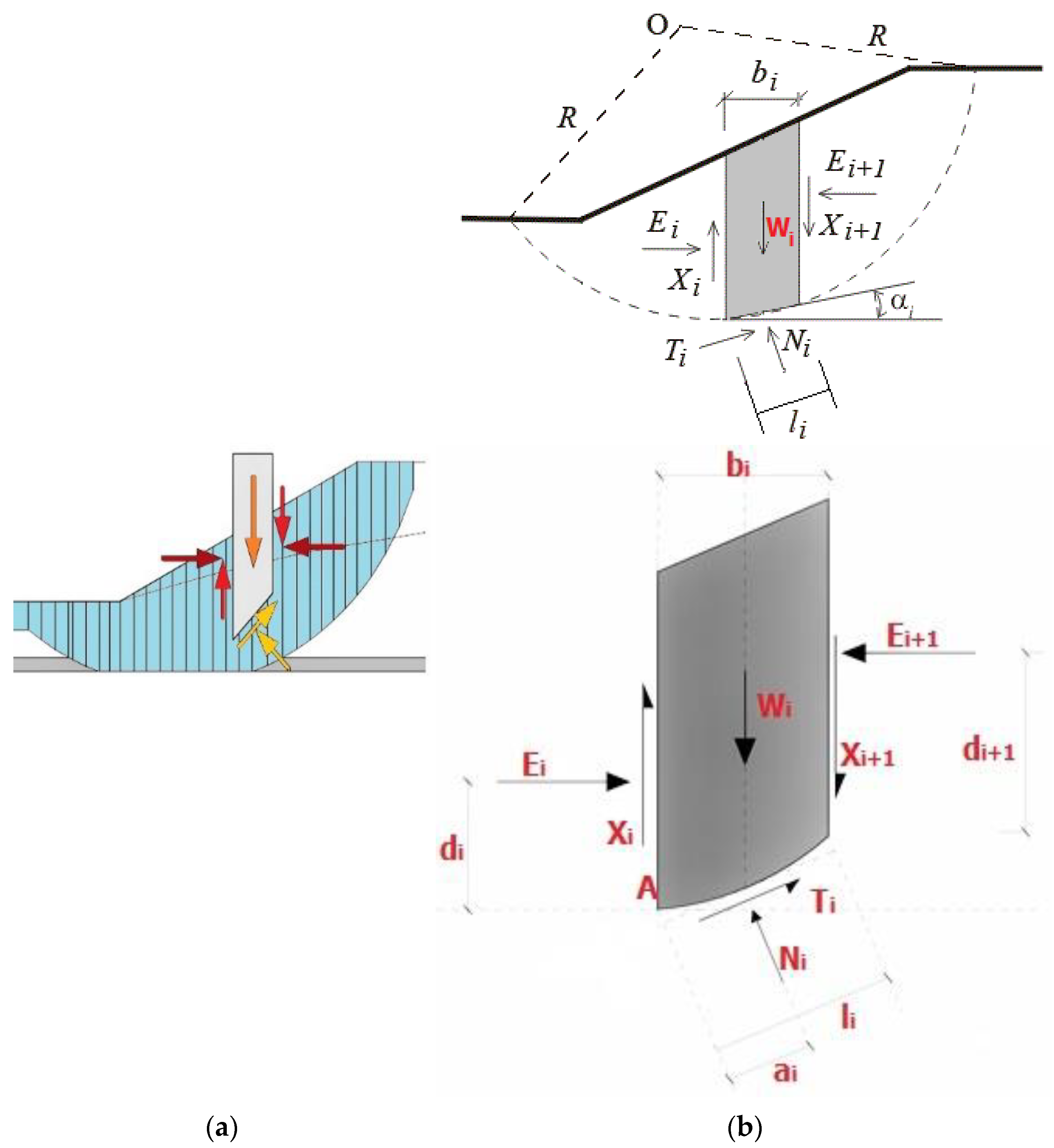
Since the block slips, the boundaries slip. Therefore, the slip surface consists of the sum points that (1) develop very slight displacements compared to the slip block and (2) are near the points with large displacements.
Picking up some of the points with a displacement very close to zero from all those points along the line separating the slip block from the unmoving soil mass, reading their coordinates, and then writing their coordinates to an Excel file required creating a table consisting of enough points supposed to define the slip surface. However, the coordinates of the centre of the circular slip surface (if it is a circle) were not yet obtained. The programme found (Xc, Yc).
Three points are enough to define a circle if all three are eligible for selection, and the surface is a circle. However, since there were errors in picking up the points (because of both the mesh and the subjective interpretation of the so-called “close to zero points”), an adjustment of the perfect circle was needed, which was achieved by applying the least-squares method.
The objective consisted of adjusting the parameters of the chosen model function to best fit data sets. The data set used in this study consists of “n” picked-up points for each case (data pairs) (xi, yi), i = 1, …, n, where ”x” is an independent variable, and ”y” is a dependent variable, with the values found by observation. The fitting of the model distribution to a data point was measured by its residual, which is defined as the difference between the observed value of the dependent variable and the fitting value predicted by the model used on the result of each equation. The least-squares method approximated the solutions, finding the optimal parameter values by minimizing the sum of squared residuals.
Table 3,
Table 4,
Table 5,
Table 6,
Table 7 and
Table 8 and
Figure 16,
Figure 17,
Figure 18,
Figure 19,
Figure 20 and
Figure 21 present the safety factors resulting from five LE methods (Slope2 Rocscience) [
3] and FEM (PLAXIS 2D). All regarded LE methods consider the slip surface to be circular. The comparative results between FEM, also considering circular slip surfaces (the benchmark), and LEM found that, commonly, the FoS are similar.
Table 3.
Results for Slope 1:1.5, H = 3.0 m, S1–S4.
Table 3.
Results for Slope 1:1.5, H = 3.0 m, S1–S4.
| Soil Type | S1 | S2 |
|---|
| Method | FoS | XC | YC | R | FoS | XC | YC | R |
|---|
| LEM (Slide) | Fellenius | 1.994 | 1.600 | 4.296 | 4.711 | 2.602 | 1.646 | 4.357 | 4.741 |
| Bishop simplified | 2.081 | 1.508 | 5.210 | 5.432 | 2.698 | 1.600 | 4.966 | 5.216 |
| Janbu corrected | 2.102 | 1.554 | 4.783 | 5.094 | 2.743 | 1.646 | 4.783 | 5.062 |
| Spencer | 2.079 | 1.508 | 5.210 | 5.432 | 2.696 | 1.600 | 4.905 | 5.170 |
| Morgenstern–Price | 2.077 | 1.508 | 5.210 | 5.432 | 2.695 | 1.600 | 4.905 | 5.170 |
| FEM (Plaxis)—circular | 2.063 | 1.374 | 5.626 | 5.919 | 2.689 | 1.558 | 5.598 | 6.048 |
| Soil Type | S3 | S4 |
| Method | FoS | XC | YC | R | FoS | XC | YC | R |
| LEM (Slide) | Fellenius | 3.314 | 1.692 | 4.357 | 4.726 | 5.203 | 1.866 | 4.513 | 6.110 |
| Bishop simplified | 3.431 | 1.646 | 4.783 | 5.062 | 5.329 | 1.720 | 4.513 | 4.834 |
| Janbu corrected | 3.495 | 1.646 | 4.783 | 5.062 | 5.521 | 1.866 | 5.123 | 6.539 |
| Spencer | 3.429 | 1.646 | 4.783 | 5.062 | 5.330 | 1.720 | 4.513 | 4.834 |
| Morgenstern–Price | 3.427 | 1.646 | 4.783 | 5.062 | 5.328 | 1.720 | 4.513 | 4.834 |
| FEM (Plaxis)—circular | 3.423 | 1.564 | 5.366 | 5.908 | 5.282 | 1.986 | 5.417 | 6.793 |
Figure 16.
FoS for Slope 1:1.5, H = 3.00 m, S1–S4.
Figure 16.
FoS for Slope 1:1.5, H = 3.00 m, S1–S4.
Table 4.
Results for slope 1:1.5, H = 8.0 m, S1 = S4.
Table 4.
Results for slope 1:1.5, H = 8.0 m, S1 = S4.
| Soil Type | S1 | S2 |
|---|
| Method | FoS | XC | YC | R | FoS | XC | YC | R |
|---|
| LEM (Slide) | Fellenius | 1.170 | 2.270 | 13.973 | 14.159 | 1.464 | 2.710 | 13.364 | 13.638 |
| Bishop simplified | 1.224 | 1.390 | 15.040 | 15.104 | 1.532 | 1.976 | 14.354 | 14.490 |
| Janbu corrected | 1.223 | 1.976 | 14.354 | 14.490 | 1.532 | 2.563 | 13.592 | 13.830 |
| Spencer | 1.222 | 1.390 | 15.040 | 15.104 | 1.528 | 1.976 | 14.354 | 14.490 |
| Morgenstern–Price | 1.221 | 1.390 | 15.040 | 15.104 | 1.528 | 1.976 | 14.354 | 14.490 |
| FEM (Plaxis) | 1.195 | 1.161 | 17.484 | 17.706 | 1.509 | 1.859 | 16.742 | 17.024 |
| Soil Type | S3 | S4 |
| Method | FoS | XC | YC | R | FoS | XC | YC | R |
| LEM (Slide) | Fellenius | 1.844 | 2.930 | 13.059 | 13.381 | 2.513 | 3.957 | 11.230 | 11.912 |
| Bishop simplified | 1.930 | 2.050 | 14.278 | 14.422 | 2.601 | 3.737 | 11.687 | 12.270 |
| Janbu corrected | 1.931 | 2.563 | 13.592 | 13.830 | 2.655 | 3.664 | 11.840 | 12.390 |
| Spencer | 1.925 | 2.050 | 14.278 | 14.422 | 2.599 | 3.590 | 11.992 | 12.510 |
| Morgenstern–Price | 1.925 | 2.050 | 14.278 | 14.422 | 2.597 | 3.737 | 11.687 | 12.270 |
| FEM (Plaxis) | 1.844 | 2.930 | 13.059 | 13.381 | 2.604 | 3.915 | 14.845 | 15.915 |
Figure 17.
FoS for Slope 1:1.5, H = 8.00 m, S1–S4.
Figure 17.
FoS for Slope 1:1.5, H = 8.00 m, S1–S4.
Table 5.
Results for slope 1:1, H = 3.0 m.
Table 5.
Results for slope 1:1, H = 3.0 m.
| Soil Type | S1 | S2 |
|---|
| Method | FoS | XC | YC | R | FoS | XC | YC | R |
|---|
| LEM (Slide) | Fellenius | 1.752 | 0.565 | 4.864 | 4.897 | 2.298 | 0.703 | 4.620 | 4.674 |
| Bishop simplified | 1.785 | 0.382 | 5.169 | 5.183 | 2.338 | 0.382 | 5.169 | 5.183 |
| Janbu corrected | 1.851 | 0.382 | 5.169 | 5.183 | 2.440 | 0.382 | 5.169 | 5.183 |
| Spencer | 1.784 | 0.382 | 5.169 | 5.183 | 2.338 | 0.382 | 5.169 | 5.183 |
| Morgenstern–Price | 1.784 | 0.382 | 5.169 | 5.183 | 2.337 | 0.382 | 5.169 | 5.183 |
| FEM (Plaxis) | 1.678 | 0.113 | 5.237 | 5.260 | 2.210 | 0.283 | 5.183 | 5.225 |
| Soil Type | S3 | S4 |
| Method | FoS | XC | YC | R | FoS | XC | YC | R |
| LEM (Slide) | Fellenius | 2.931 | 0.703 | 4.620 | 4.674 | 4.707 | 0.978 | 4.071 | 4.190 |
| Bishop simplified | 2.980 | 0.565 | 4.864 | 4.897 | 4.738 | 0.978 | 4.071 | 4.190 |
| Janbu corrected | 3.116 | 0.382 | 5.169 | 5.183 | 5.106 | 0.565 | 4.864 | 4.897 |
| Spencer | 2.980 | 0.565 | 4.864 | 4.897 | 4.878 | 0.290 | 5.291 | 5.306 |
| Morgenstern–Price | 2.978 | 0.565 | 4.864 | 4.897 | 4.794 | 0.428 | 5.108 | 5.121 |
| FEM (Plaxis) | 2.821 | 0.334 | 5.159 | 5.195 | 4.489 | 0.782 | 5.210 | 5.325 |
Figure 18.
FoS for Slope 1:1, H = 3.00 m, S1–S4.
Figure 18.
FoS for Slope 1:1, H = 3.00 m, S1–S4.
Table 6.
Results for slope 1:1, H = 8.0 m.
Table 6.
Results for slope 1:1, H = 8.0 m.
| Soil Type | S1 | S2 |
|---|
| Method | FoS | XC | YC | R | FoS | XC | YC | R |
|---|
| LEM (Slide) | Fellenius | 0.962 | −0.754 | 12.235 | 12.255 | 1.222 | −0.020 | 11.778 | 11.771 |
| Bishop simplified | 0.994 | −1.047 | 12.388 | 12.431 | 1.258 | −0.387 | 12.007 | 12.011 |
| Janbu corrected | 1.011 | −0.901 | 12.311 | 12.343 | 1.287 | −0.387 | 12.007 | 12.011 |
| Spencer | 0.992 | −1.047 | 12.388 | 12.431 | 1.256 | −0.387 | 12.007 | 12.011 |
| Morgenstern−Price | 0.992 | −0.974 | 12.388 | 12.413 | 1.255 | −0.460 | 12.083 | 12.081 |
| FEM (Plaxis) | 0.947 | −2.204 | 15.199 | 15.376 | 1.190 | −1.716 | 14.472 | 14.705 |
| Soil Type | S3 | S4 |
| Method | FoS | XC | YC | R | FoS | XC | YC | R |
| LEM (Slide) | Fellenius | 1.545 | −0.020 | 11.778 | 11.771 | 2.193 | 1.464 | 10.518 | 11.016 |
| Bishop simplified | 1.589 | −0.387 | 12.007 | 12.011 | 2.227 | 0.950 | 10.975 | 11.016 |
| Janbu corrected | 1.630 | −0.387 | 12.007 | 12.011 | 2.353 | 0.143 | 14.785 | 14.786 |
| Spencer | 1.588 | −0.387 | 12.007 | 12.011 | 2.222 | 1.317 | 10.670 | 10.736 |
| Morgenstern−Price | 1.586 | −0.387 | 12.007 | 12.011 | 2.227 | 0.950 | 10.975 | 11.016 |
| FEM (Plaxis) | 1.501 | −1.315 | 13.789 | 13.944 | 2.130 | 0.032 | 14.438 | 14.537 |
Figure 19.
FoS for Slope 1:1, H = 8.00 m, S1–S4.
Figure 19.
FoS for Slope 1:1, H = 8.00 m, S1–S4.
Table 7.
Results for slope 2:1, H = 3.0 m.
Table 7.
Results for slope 2:1, H = 3.0 m.
| Soil Type | S1 | S2 |
|---|
| Method | FoS | XC | YC | R | FoS | XC | YC | R |
|---|
| LEM (Slide) | Fellenius | 1.405 | −1.350 | 4.681 | 4.866 | 1.869 | −1.029 | 4.437 | 4.554 |
| Bishop simplified | 1.396 | −1.350 | 4.681 | 4.866 | 1.853 | −1.029 | 4.437 | 4.554 |
| Janbu corrected | 1.512 | −1.625 | 4.864 | 5.122 | 2.034 | −1.533 | 4.803 | 5.036 |
| Spencer | 1.639 | −2.166 | 7.790 | 7.873 | 2.203 | −0.799 | 7.729 | 7.768 |
| Morgenstern−Price | 1.631 | −1.212 | 7.790 | 7.881 | 2.186 | 0.576 | 2.365 | 2.672 |
| FEM (Plaxis) | 1.389 | −1.473 | 5.429 | 5.666 | 1.860 | −1.267 | 5.293 | 5.481 |
| Soil Type | S3 | S4 |
| Method | FoS | XC | YC | R | FoS | XC | YC | R |
| LEM (Slide) | Fellenius | 2.392 | −1.029 | 4.437 | 4.554 | 3.985 | −0.799 | 4.254 | 4.328 |
| Bishop simplified | 2.371 | −1.029 | 4.437 | 4.554 | 3.941 | −0.249 | 3.767 | 3.772 |
| Janbu corrected | 2.610 | −1.441 | 4.742 | 4.951 | 4.421 | −1.808 | 7.851 | 8.052 |
| Spencer | 2.812 | 0.668 | 2.243 | 2.565 | 4.752 | −0.020 | 7.546 | 7.549 |
| Morgenstern−Price | 2.790 | 0.622 | 2.304 | 2.618 | 4.635 | 0.255 | 1.938 | 2.702 |
| FEM (Plaxis) | 2.379 | −1.268 | 5.424 | 5.612 | 3.970 | −0.535 | 4.955 | 5.106 |
Figure 20.
FoS for Slope 2:1, H = 3.00 m, S1–S4.
Figure 20.
FoS for Slope 2:1, H = 3.00 m, S1–S4.
Table 8.
Results for slope 2:1, H = 8.0 m.
Table 8.
Results for slope 2:1, H = 8.0 m.
| Soil Type | S1 | S2 |
|---|
| Method | FoS | XC | YC | R | FoS | XC | YC | R |
|---|
| LEM (Slide) | Fellenius | 0.745 | −4.059 | 10.172 | 10.951 | 0.961 | −3.619 | 10.324 | 10.934 |
| Bishop simplified | 0.741 | −2.959 | 8.724 | 9.211 | 0.951 | −2.812 | 8.724 | 9.160 |
| Janbu corrected | 0.792 | −4.573 | 11.544 | 12.404 | 1.022 | −4.426 | 11.620 | 12.433 |
| Spencer | 0.762 | −4.206 | 11.848 | 12.544 | 1.007 | −3.106 | 12.382 | 12.759 |
| Morgenstern−Price | 0.766 | −3.986 | 11.925 | 12.565 | 1.009 | −3.106 | 12.458 | 12.806 |
| FEM (Plaxis) | 0.598 | −7.835 | 17.389 | 19.126 | 0.886 | −7.202 | 16.031 | 17.663 |
| Soil Type | S3 | S4 |
| Method | FoS | XC | YC | R | FoS | XC | YC | R |
| LEM (Slide) | Fellenius | 1.219 | −4.426 | 11.620 | 12.433 | 1.803 | −1.749 | 10.461 | 10.605 |
| Bishop simplified | 1.206 | −2.739 | 8.724 | 9.134 | 1.762 | −1.162 | 8.327 | 8.407 |
| Janbu corrected | 1.299 | −4.426 | 11.620 | 12.433 | 1.956 | −2.996 | 12.442 | 12.788 |
| Spencer | 1.290 | −2.812 | 12.534 | 12.833 | 2.038 | 0.085 | 13.509 | 13.504 |
| Morgenstern−Price | 1.285 | −2.886 | 12.534 | 12.838 | 2.015 | −0.135 | 13.509 | 13.487 |
| FEM (Plaxis) | 1.171 | −7.384 | 15.778 | 17.502 | 1.786 | −3.974 | 14.841 | 15.487 |
Figure 21.
FoS for Slope 2:1, H = 8.00 m, S1–S4.
Figure 21.
FoS for Slope 2:1, H = 8.00 m, S1–S4.
Knowledge of the critical slip surface profile beneath the landslide is essential for stability analysis and design of remedial works. Hence, the study selected different models for the slip surface and utilized the measurements of displacements performed in FEM to forecast the position and shape of the slip surface, accepting that this surface is not necessarily circular.
By observation, the study selected three distinct models for the potential slip surface, i.e., a damped sinusoid, a second-degree parabola, and a logarithmic spiral determined by both polar and Cartesian coordinates, by using the same picked-up points as for the circular slip surfaces already defined in each case investigated, which were considered benchmarks for these models.
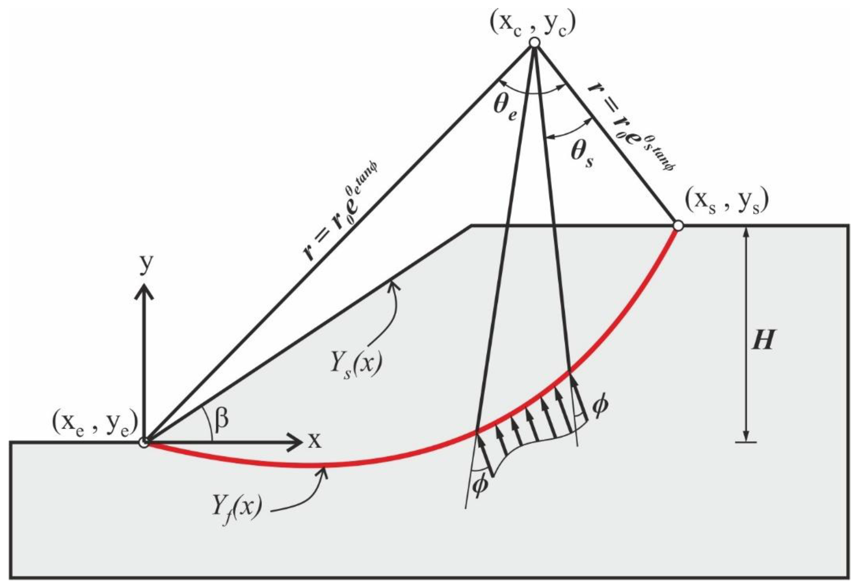
Figure 22 shows a log-spiral failure curve and the associated parameters used in the current characterization. Functions Y
s(x) and Y
f(x) describe slope surface and failure surface, respectively. Y
f(x) corresponds to a log spiral, described by ‘r’ in polar coordinates. Coordinates (Xc, Yc) represent the pole of the log spiral of the Cartesian system with the origin at the toe of the slope. That is the reason why (Xs, Ys) and (Xe, Ye) are the coordinates at which the failure surface intersects the slope surface, associated with angles θs and θe of polar coordinates [
33]. The log-spiral failure surface predicts the critical failure surface of different 2D slope geometries studied using an optimization process.
The equations corresponding to the three types of slip surface models are the following:
where r is the spiral radius (i.e., distance from the pole to the failure surface),
is the radius value for = 0°, and
is the friction angle of the material.
The most efficient approach for finding coefficients that minimize the error for these models was also to use least-squares optimization.
Table 9 presents the fitting parameters for the damped sinusoid and second-degree parabola for all cases considered, necessary to plot a potential critical slip surface as close as possible to that determined by the picked-up points.
Then, the study found the fitting parameters for the log spiral using the same optimization method, with slight differences in the results achieved in polar coordinates compared to those obtained in the Cartesian system in all cases. Then, the study compared the values of the fitting errors for each type of slip surface investigated with the fitting errors of the classical circular benchmark slip surface calculated above (
Table 10).
Figure 23a–c shows the graphs of the regression curves for five distinct shapes of the potential slip surface, including the benchmark (the circular slip surface) for three different slope gradients and H = 3, S1.
The results in
Figure 23 show that, as expected, the logarithmic spiral seems to fit best for 1:1.5 and 1:1 slopes, while, unexpectedly, the optimal shape for 2:1 steep slopes is a damped sinusoid. However, the parabola seems to verify some cases quite well. The circular surface does not seem to confirm any case taken into account.


