
Optimization Models of Actuated Control Considering Vehicle Queuing for Sustainable Operation


Abstract
:1. Introduction
2. Literature Review
3. Vehicle Queuing Model Based on Improved Traffic Wave Model
3.1. Improved Traffic Wave Model
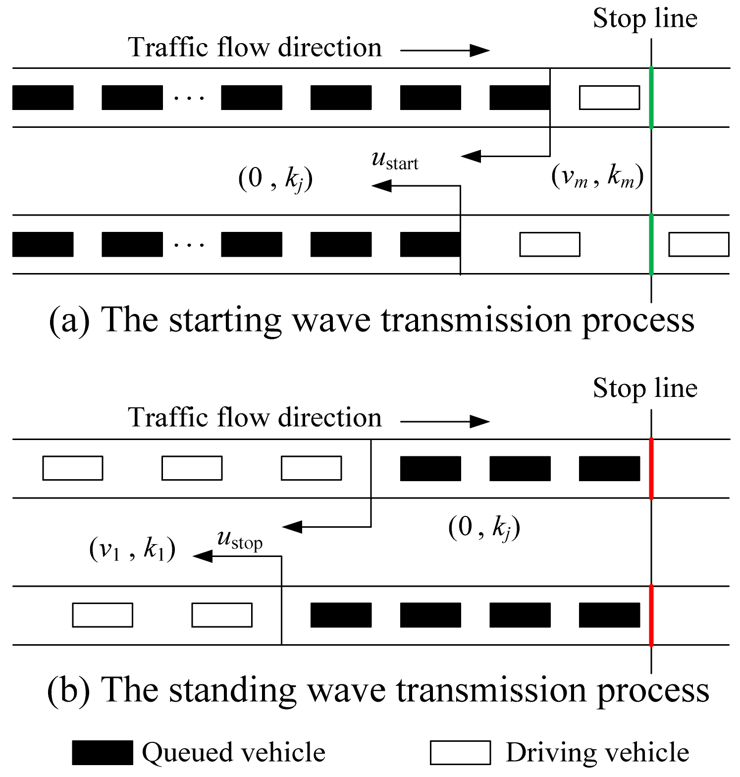
3.2. Vehicle Queuing and Dispersion Process
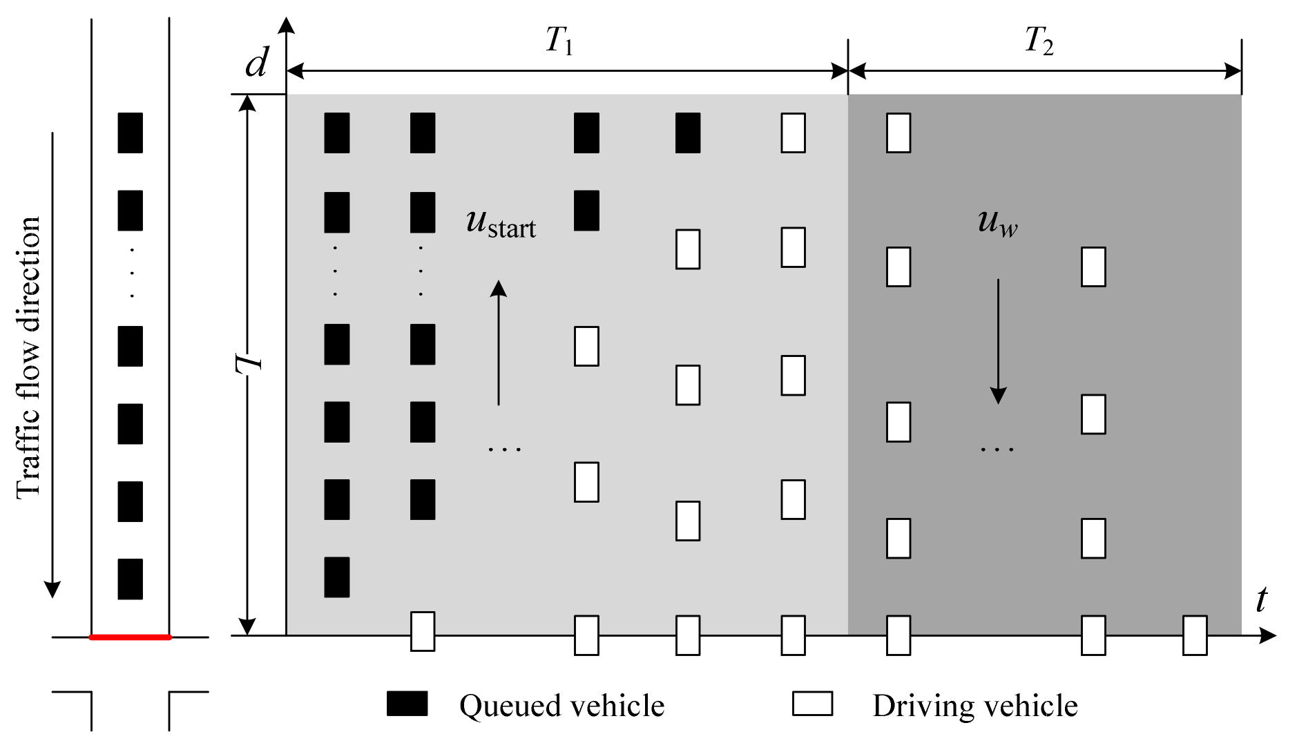
3.2.1. Vehicle Queuing Process
3.2.2. Vehicle Dispersion Process
3.3. Vehicle-Queuing Model
4. Optimization Models of Basic Parameters
4.1. Minimal Green Time Optimization Model
4.2. Maximal Green Time Optimization Model
5. Solving Algorithm for the Optimization Model
5.1. Variable Coding
5.2. Fitness Function
5.3. Genetic Manipulation
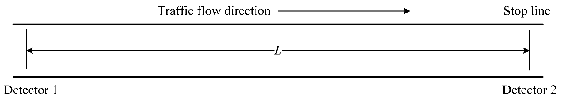
6. Verification
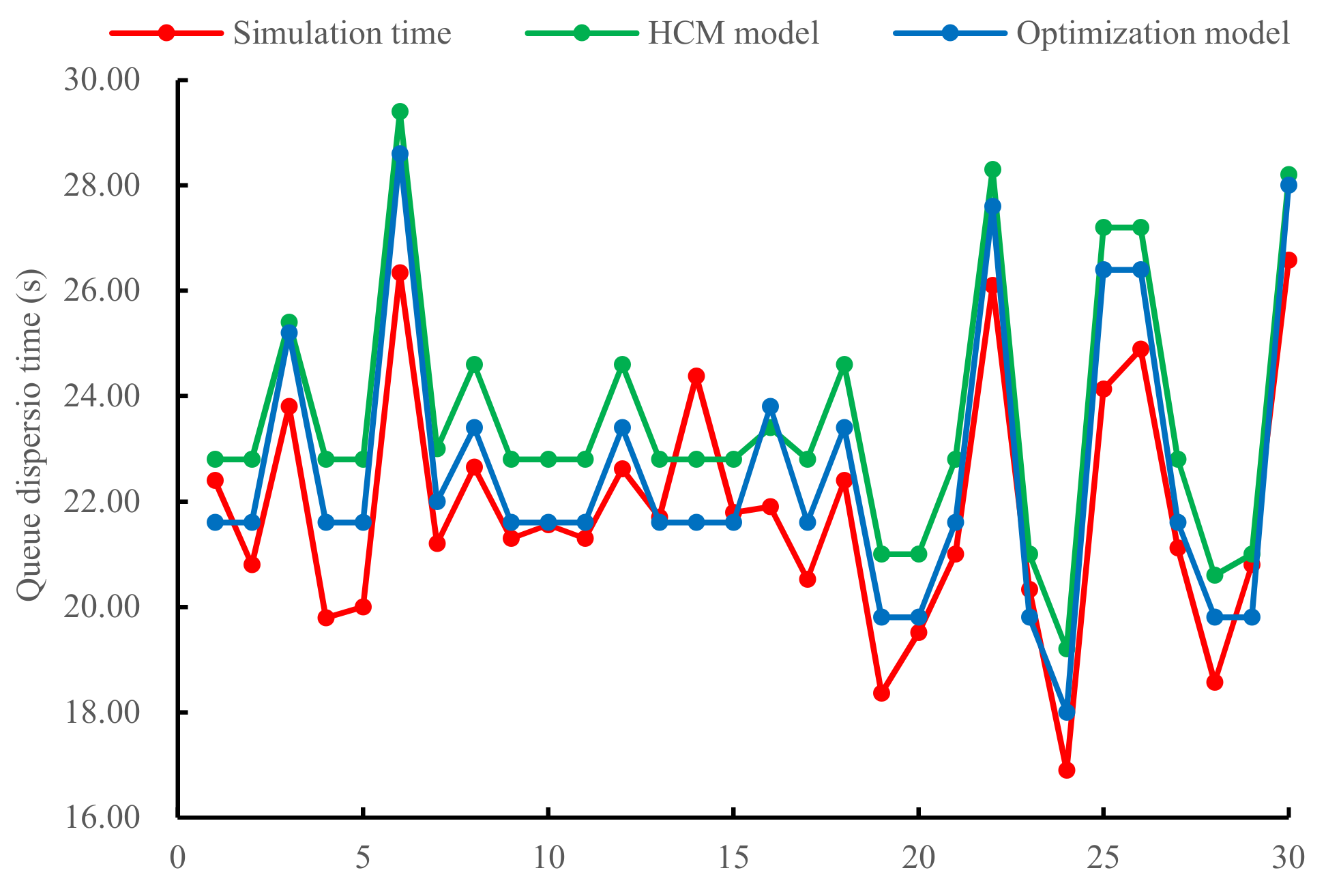
6.1. Verification of Minimal Green Time Calculation Model
6.2. Verification of Maximal Green Time Calculation Model
7. Conclusions
Author Contributions
Funding
Institutional Review Board Statement
Informed Consent Statement
Data Availability Statement
Conflicts of Interest
References
- Downs, A. The law of peak-hour expressway congestion. Traffic 1962, 33, 347–362. [Google Scholar]
- Wang, Z.L. Multimodal Traffic Adaptive Signal Control Based on Deep Reinforcement Learning. Ph.D. Thesis, Southeast University, Nanjing, China, 2021. [Google Scholar]
- Han, Y. Research on Signal Optimization in Controlled Intersections Based on Deep Reinforcement Learning. Master’s Thesis, Beijing Jiaotong University, Beijing, China, 2021. [Google Scholar]
- Liu, J.J.; Zuo, X.Q. Research on fuzzy control and optimization for traffic lights at signal intersection. J. Syst. Simul. 2020, 32, 2401–2408. [Google Scholar]
- Xing, Y.; Hao, Y.Q.; Gao, Z.J.; Liu, W.D.; Li, Z.Z. Signal timing optimization of signal intersection based on fuzzy logic. China Sci. Pap. 2021, 16, 890–894. [Google Scholar]
- Cao, Y. Optimization of adaptive signal control using simulated annealing algorithm. J. Transp. Eng. Inf. 2018, 16, 49–55+60. [Google Scholar]
- Yan, L.P.; Zhang, M.K.; Guo, C.Y.; Zhu, L.L. Real time multi-intersection signal control based on quantum particle swarm optimization. Comput. Simul. 2021, 38, 180–184. [Google Scholar]
- AMAP. 2020 Traffic Analysis Report of China’s Major Cities. 2020. Available online: https://recordtrend.com/research-report/2020-traffic-analysis-report-of-major-cities-in-china-from-gaud-map/ (accessed on 16 November 2021).
- Zhou, T.M. Research on optimal design of intersection actuated signal control. J. Chin. People’s Public Secur. Univ. 2001, 2, 34–37. [Google Scholar]
- Webster, F.V. Traffic signal settings. In Road Research Technical Paper; HM Stationery Office: London, UK, 1958. [Google Scholar]
- Pappis, C.P.; Mamdani, E.H. A fuzzy logic controller for a traffic junction. IEEE Trans. Syst. Man Cybern. 1977, 7, 707–717. [Google Scholar] [CrossRef]
- Murat, Y.S.; Gedizioglu, E. A fuzzy logic multi-phase signal control model for isolate junctions. Transp. Res. Part C 2005, 13, 19–36. [Google Scholar] [CrossRef]
- Cowan, R. An improved model for signalized intersections with vehicle-actuated control. J. Appl. Probab. 1978, 15, 384–396. [Google Scholar] [CrossRef]
- Akcelik, R. Estimation of green times and cycle time for vehicle-actuated signals. Transp. Res. Rec. J. Transp. Res. Board 1994, 1457, 63–72. [Google Scholar]
- Furth, P.; Cesme, B.; Muller, T. Lost time and cycle length for actuated traffic signal. Transp. Res. Rec. J. Transp. Res. Board 2009, 2128, 152–160. [Google Scholar] [CrossRef] [Green Version]
- Viti, F.; van Zuylen, H.J. A Probabilistic model for traffic at actuated control signals. Transp. Res. Part C 2010, 8, 299–310. [Google Scholar] [CrossRef]
- Moghimi, B.; Safikhani, A.; Kamga, C.; Hao, W. Cycle-length prediction in actuated traffic-signal control using ARIMA model. J. Comput. Civ. Eng. 2018, 32, 04017083. [Google Scholar] [CrossRef]
- Shiri, M.; Maleki, H. Maximum green time settings for traffic-actuated signal control at isolated intersections using fuzzy logic. Int. J. Fuzzy Syst. 2017, 19, 247–256. [Google Scholar] [CrossRef]
- Jing, T. Research on Optimization of Single Intersection Actuated Control under Stochastic Conditions. Master’s Thesis, Lanzhou Jiaotong University, Lanzhou, China, 2014. [Google Scholar]
- Hao, P.; Wu, G.; Boriboonsomsin, K.; Barth, M.J. Developing a framework of eco-approach and departure application for actuated signal control. In Proceedings of the 2015 IEEE Intelligent Vehicles Symposium (IV), Seoul, Korea, 28 June–1 July 2015. [Google Scholar]
- Bao, L.J. Traffic Signal Actuation Strategy Based on RFID. Master’s Thesis, Shanghai Institute of Technology, Shanghai, China, 2016. [Google Scholar]
- Jauregui, C.; Torres, M.; Silvera, M.; Campos, F. Improving people’s accessibility through a fully actuated signal control at intersections with high density of pedestrians. In Proceedings of the 2020 Congreso Internacional de Innovación y Tendencias en Ingeniería (CONIITI), Bogota, Colombia, 30 September–2 October 2020. [Google Scholar]
- Wang, M.; Zhang, Y.; Ding, H. Research on real-time actuated signal control of intersection based on Internet of things technology. J. Gansu Sci. 2021, 33, 98–103. [Google Scholar]
- Wu, X.; Adhikari, B.; Chiu, S.; Yang, H.; Sajjadi, S.; Roy, U. Volume-occupancy-based actuated signal control system: Design and implementation to diamond interchanges in Houston. Int. J. Civ. Eng. 2022, 20, 337–348. [Google Scholar] [CrossRef]
- Gartner, N.H.; Messer, C.J.; Rathi, A.K. Revised Monograph on Traffic Flow Theory: A State-of-the-Art Report; The Federal Highway Administration (FHWA): Washington, DC, USA, 2005. [Google Scholar]
- Zhang, H.M. A theory of nonequilibrium traffic flow. Transp. Res. Part B 1998, 32, 485–498. [Google Scholar] [CrossRef]
- Lighthill, M.J.; Whitham, G.B. On kinematic waves I: Flow movement in long rivers. Proc. R. Soc. London. Ser. A Math. Phys. Sci. 1995, 229, 281–316. [Google Scholar]
- Lighthill, M.J.; Whitham, G.B. On kinematic waves II: A theory of traffic flow on long crowded roads. Proc. R. Soc. London. Ser. A Math. Phys. Sci. 1995, 22, 317–345. [Google Scholar]
- Xu, H.F.; Liu, S.; Zhang, D.; Zheng, Q.M. Configuring parameters of fully actuated control at isolated signalized intersections. J. Jilin Univ. Eng. Technol. Ed. 2019, 49, 45–52. [Google Scholar]
- Feng, S.L. Research on Signal Timing Optimization of Isolated Intersection Based on Multi-Phase Variable Phase Sequence. Master’s Thesis, Lanzhou Jiaotong University, Lanzhou, China, 2014. [Google Scholar]
- NEMA. NEMA Standards Publication TS-2; NEMA: Nairobi, Kenya, 2003. [Google Scholar]
- Cao, C.T.; Xu, J.M. Multi-object traffic signal control method for single intersection. Comput. Eng. Appl. 2010, 46, 20–22. [Google Scholar]


| Phase Schemes | Schematic Diagrams |
|---|---|
| F1 |  |
| F2 | 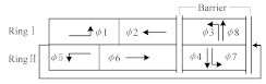 |
| F3 | 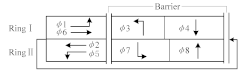 |
| F4 | 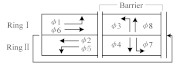 |
| Phase Schemes | Objective Function and Constraints | |
|---|---|---|
| F1 | Delay | |
| Capacity | ||
| Constraints | ||
| F2 | Delay | |
| Capacity | ||
| Constraints | ||
| F3 | Delay | |
| Capacity | ||
| Constraints | ||
| F4 | Delay | |
| Capacity | ||
| Constraints | ||
| Index | Simulation Time (s) | HCM Model (s) | Relative Error | Optimization Model (s) | Relative Error |
|---|---|---|---|---|---|
| 1 | 22.40 | 22.80 | 1.79% | 21.60 | 3.57% |
| 2 | 20.80 | 22.80 | 9.62% | 21.60 | 3.85% |
| 3 | 23.80 | 25.40 | 6.72% | 25.20 | 5.88% |
| 4 | 19.79 | 22.80 | 15.21% | 21.60 | 9.15% |
| 5 | 20.00 | 22.80 | 14.00% | 21.60 | 8.00% |
| 6 | 26.34 | 29.40 | 11.62% | 28.60 | 8.58% |
| 7 | 21.20 | 23.00 | 8.49% | 22.00 | 3.77% |
| 8 | 22.65 | 24.60 | 8.61% | 23.40 | 3.31% |
| 9 | 21.30 | 22.80 | 7.04% | 21.60 | 1.41% |
| 10 | 21.56 | 22.80 | 5.75% | 21.60 | 0.19% |
| 11 | 21.30 | 22.80 | 7.04% | 21.60 | 1.41% |
| 12 | 22.62 | 24.60 | 8.75% | 23.40 | 3.45% |
| 13 | 21.70 | 22.80 | 5.07% | 21.60 | 0.46% |
| 14 | 24.38 | 22.80 | 6.48% | 21.60 | 11.40% |
| 15 | 21.79 | 22.80 | 4.64% | 21.60 | 0.87% |
| 16 | 21.90 | 23.40 | 6.85% | 23.80 | 8.68% |
| 17 | 20.52 | 22.80 | 11.11% | 21.60 | 5.26% |
| 18 | 22.40 | 24.60 | 9.82% | 23.40 | 4.46% |
| 19 | 18.36 | 21.00 | 14.38% | 19.80 | 7.84% |
| 20 | 19.51 | 21.00 | 7.64% | 19.80 | 1.49% |
| 21 | 21.00 | 22.80 | 8.57% | 21.60 | 2.86% |
| 22 | 26.10 | 28.30 | 8.43% | 27.60 | 5.75% |
| 23 | 20.33 | 21.00 | 3.30% | 19.80 | 2.61% |
| 24 | 16.90 | 19.20 | 13.61% | 18.00 | 6.51% |
| 25 | 24.13 | 27.20 | 12.72% | 26.40 | 9.41% |
| 26 | 24.89 | 27.20 | 9.28% | 26.40 | 6.07% |
| 27 | 21.12 | 22.80 | 7.95% | 21.60 | 2.27% |
| 28 | 18.57 | 20.60 | 10.93% | 19.80 | 6.62% |
| 29 | 20.80 | 21.00 | 0.96% | 19.80 | 4.81% |
| 30 | 26.58 | 28.20 | 6.09% | 28.00 | 5.34% |
| Queue Length (m) | Simulation Time (s) | HCM Model | Optimization Model | ||
|---|---|---|---|---|---|
| Time (s) | Relative Error | Time (s) | Relative Error | ||
| 25 | 9.92 | 11.56 | 18.13% | 10.06 | 3.90% |
| 35 | 12.01 | 13.20 | 10.41% | 12.13 | 3.39% |
| 45 | 18.41 | 19.73 | 7.29% | 19.13 | 3.83% |
| 55 | 21.82 | 23.54 | 8.42% | 22.53 | 4.84% |
| 65 | 24.54 | 26.17 | 7.94% | 25.22 | 4.91% |
| Average relative error | 10.44% | 4.18% | |||
| Traffic Flow Direction | Traffic Volume (pcu/h) | Saturated Flow (pcu/h) | Ratio | |
|---|---|---|---|---|
| SB | TH | 912 | 2750 | 0.33 |
| LT | 356 | 1550 | 0.23 | |
| NB | TH | 832 | 2750 | 0.30 |
| LT | 144 | 1550 | 0.09 | |
| WB | TH | 288 | 2450 | 0.08 |
| LT | 428 | 2150 | 0.20 | |
| EB | TH | 248 | 2750 | 0.09 |
| LT | 216 | 1550 | 0.14 | |
| Phase Schemes | Index | WB LT (s) | B TH (s) | NB LT (s) | SB TH (s) | EB LT (s) | WB TH (s) | SB LT (s) | NB TH (s) |
|---|---|---|---|---|---|---|---|---|---|
| F1 | ① | 32 | 15 | 37 | 54 | 32 | 15 | 37 | 54 |
| ② | 18 | 22 | 20 | 53 | 17 | 23 | 20 | 53 | |
| F2 | ① | 24 | 10 | 39 | 39 | 24 | 10 | 39 | 39 |
| ② | 25 | 15 | 36 | 36 | 14 | 26 | 36 | 36 | |
| F3 | ① | 16 | 16 | 18 | 24 | 16 | 16 | 18 | 24 |
| ② | 13 | 13 | 12 | 36 | 13 | 13 | 22 | 26 | |
| F4 | ① | 12 | 12 | 20 | 20 | 12 | 12 | 20 | 20 |
| ② | 10 | 10 | 22 | 22 | 10 | 10 | 22 | 22 |
| Phase Schemes | Index | Average Vehicle Delay (s) | Traffic Capacity (pcu/h) | Optimization Ratio |
|---|---|---|---|---|
| F1 | ① | 59.62 | 4279 | / |
| ② | 42.69 | 4472 | 12.79% | |
| F2 | ① | 24.75 | 3185 | / |
| ② | 24.15 | 3742 | 10.75% | |
| F3 | ① | 26.07 | 3328 | / |
| ② | 22.57 | 3741 | 11.45% | |
| F4 | ① | 7.84 | 7733 | / |
| ② | 7.57 | 7668 | 2.10% | |
| Average optimization ratio | 9.27% | |||
Publisher’s Note: MDPI stays neutral with regard to jurisdictional claims in published maps and institutional affiliations. |
© 2022 by the authors. Licensee MDPI, Basel, Switzerland. This article is an open access article distributed under the terms and conditions of the Creative Commons Attribution (CC BY) license (https://creativecommons.org/licenses/by/4.0/).
Share and Cite
Wang, X.; Wu, X.; Liu, J. Optimization Models of Actuated Control Considering Vehicle Queuing for Sustainable Operation. Sustainability 2022, 14, 8998. https://doi.org/10.3390/su14158998
Wang X, Wu X, Liu J. Optimization Models of Actuated Control Considering Vehicle Queuing for Sustainable Operation. Sustainability. 2022; 14(15):8998. https://doi.org/10.3390/su14158998
Chicago/Turabian StyleWang, Xinyue, Xianyu Wu, and Jiarui Liu. 2022. "Optimization Models of Actuated Control Considering Vehicle Queuing for Sustainable Operation" Sustainability 14, no. 15: 8998. https://doi.org/10.3390/su14158998