

Temporal Segmentation for the Estimation and Benchmarking of Heating and Cooling Energy in Commercial Buildings in Seoul, South Korea

Abstract
:1. Introduction
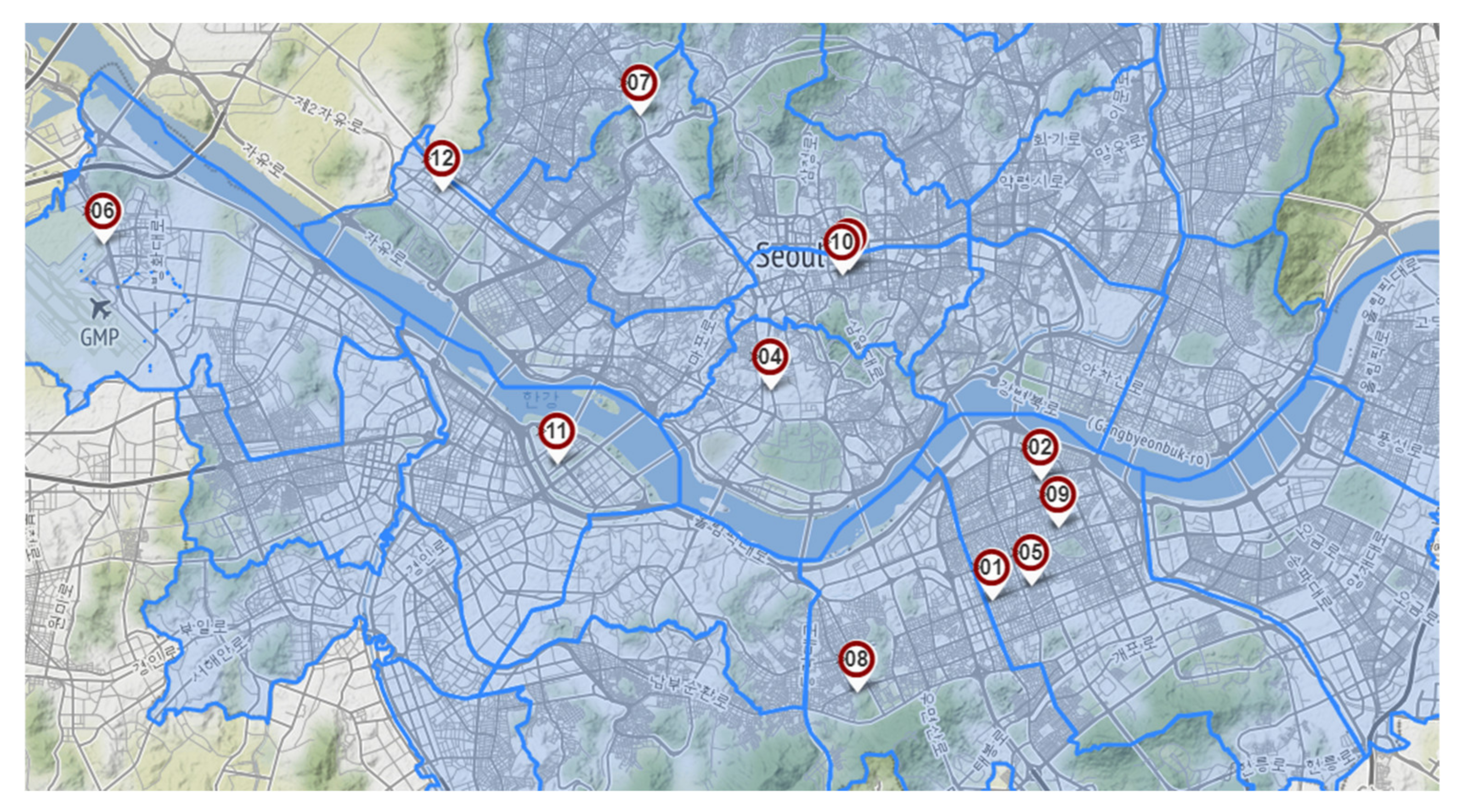
2. Data
- Cooling energy (Cool): energy used for space cooling in the building through central cooling sources (e.g., chiller, cooling tower), pumps involved in cooling, individual cooling systems (e.g., electric heat pumps, gas heat pumps), and their operation and control.
- Heating energy (Heat): energy used for space heating in the building through central heating sources (e.g., boiler), pumps involved in heating, individual heating systems (e.g., electric heat pumps, gas heat pumps), and their operation and control.
- Hot water supply (Shw): energy used to produce and transport hot water for building domestic water services by central hot water sources (e.g., boilers) and pumps carrying hot water.
- Lighting (Light): Energy used by the main lighting equipment composed of separated branch circuits.
- Air movement by fan (Vent): energy used for cooling, heating, ventilation, and air circulation by fans in mechanical systems (e.g., air handling unit, outdoor unit, fan coil unit).
- Appliances (App): energy used by office appliances, auxiliary heaters, electric fans, water purifiers, and non-identifiable energy use in circuits.
- Indoor transportation (Trans): energy used by indoor transportation devices (e.g., escalators, lifts, etc.)
- Auxiliary devices (Aux): energy used by main pumps for water supply.
3. Methods
3.1. Information Gain-Based Temporal Segmentation (IGTS)
3.2. Estimation of Cooling and Heating Energy
4. Results
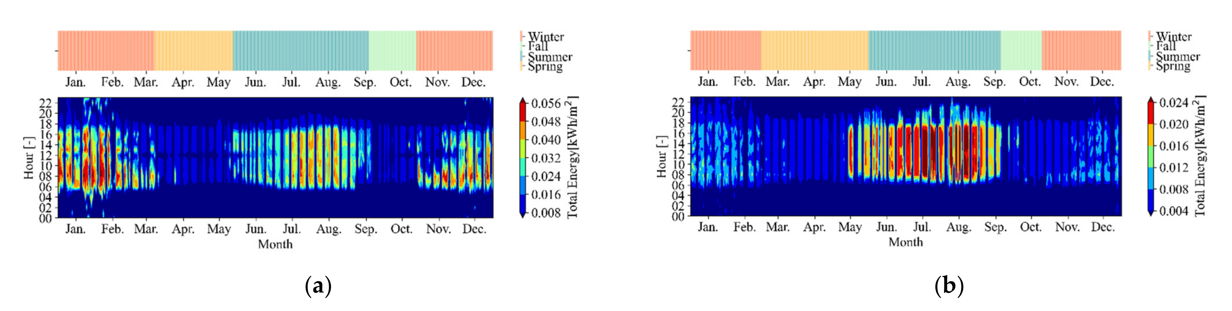
4.1. Temporal Segmentation for Estimation of Heating and Cooling Energy
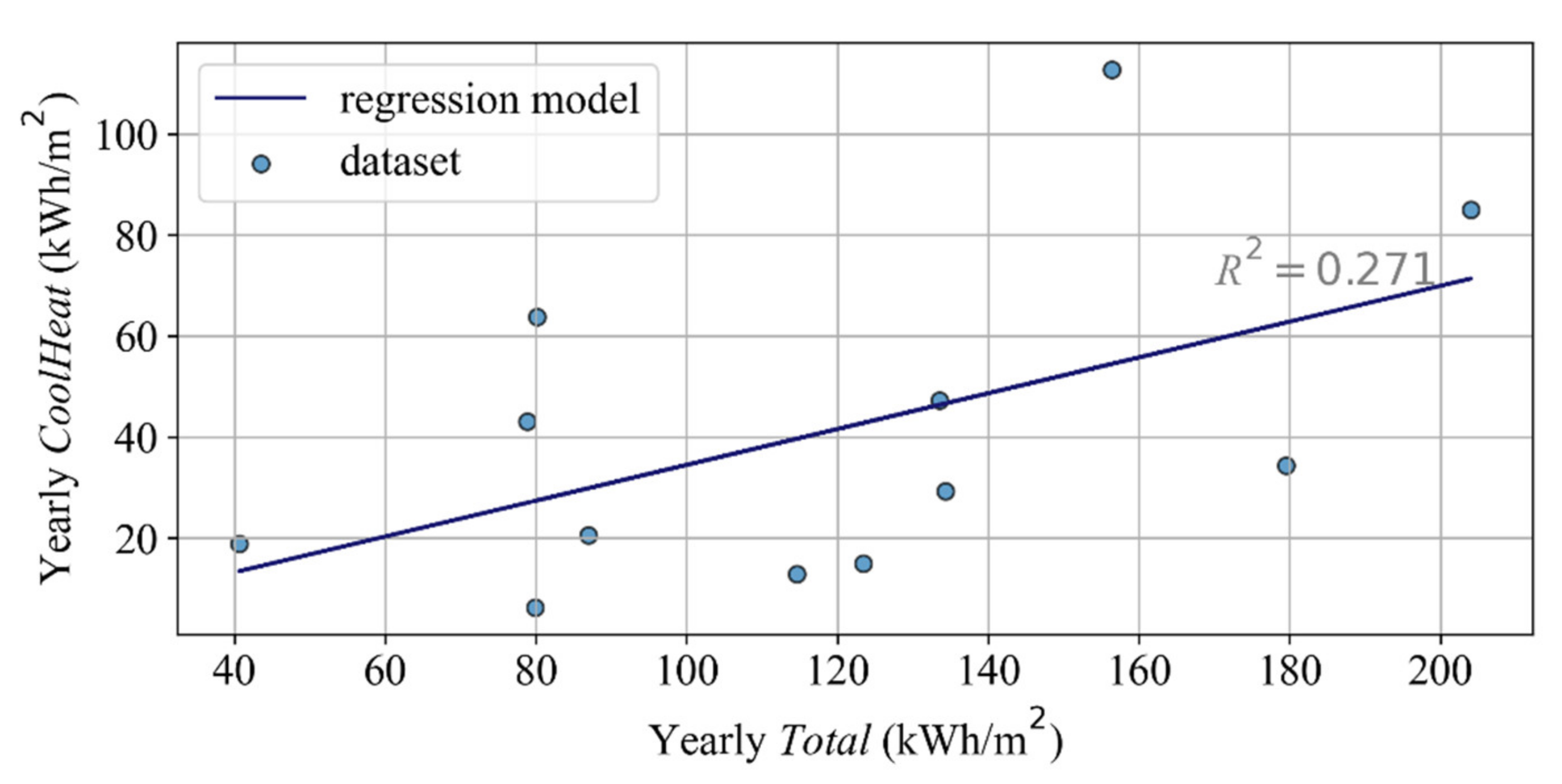
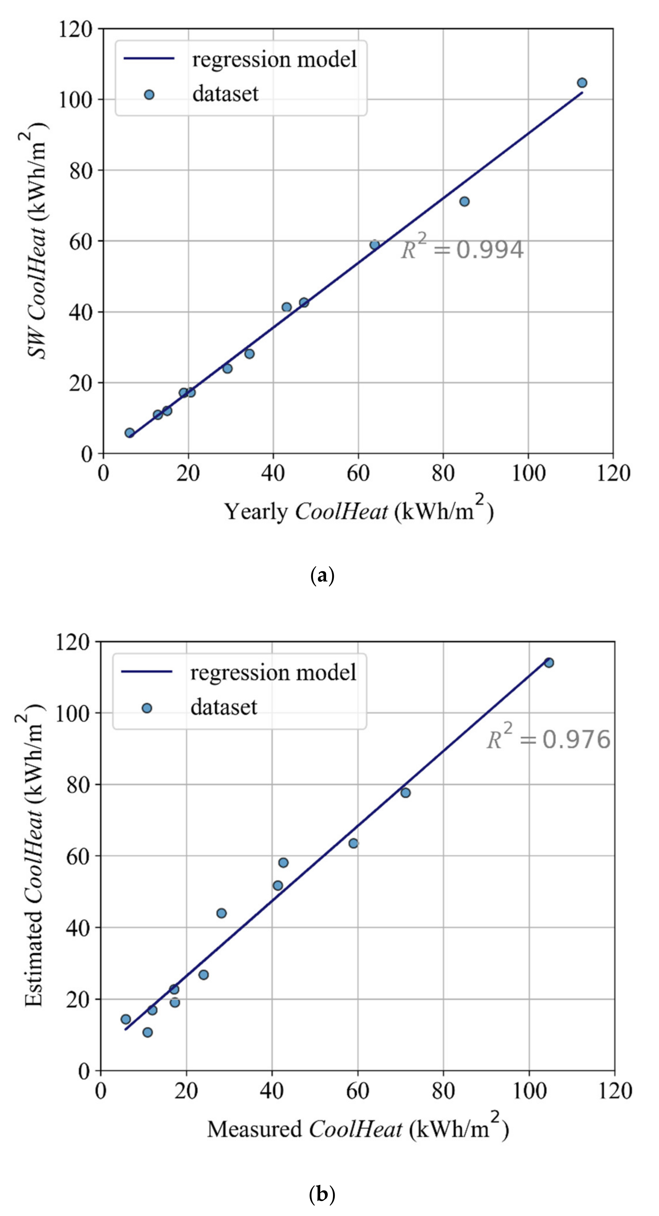
4.2. Benchmarking Based on Estimated Heating and Cooling Energy
5. Limitations
6. Conclusions
Author Contributions
Funding
Institutional Review Board Statement
Data Availability Statement
Conflicts of Interest
References
- Kim, D.W.; Kim, Y.M.; Lee, S.E. Development of an energy benchmarking database based on cost-effective energy performance indicators: Case study on public buildings in South Korea. Energy Build 2019, 191, 104–116. [Google Scholar] [CrossRef]
- Korea.net. Available online: https://www.korea.net/NewsFocus/policies/view?articleId=205222 (accessed on 9 June 2022).
- Korea.kr. Available online: https://www.korea.kr/news/policyNewsView.do?newsId=148894861 (accessed on 9 June 2022).
- Chung, W.; Hui, Y.V.; Lam, M. Benchmarking the energy efficiency of commercial buildings. Appl. Energy 2006, 83, 1–14. [Google Scholar] [CrossRef]
- Chung, W. Review of building energy-use performance benchmarking methodologies. Appl. Energy 2011, 88, 1470–1479. [Google Scholar] [CrossRef]
- Pérez-Lombard, L.; Ortiz, J.; González, R.; Maestre, I.R. A review of benchmarking, rating and labelling concepts within the framework of building energy certification schemes. Energy Build 2009, 41, 272–278. [Google Scholar] [CrossRef]
- CIBSE, TM46; Energy Benchmarks. The Chartered Institution of Building Services Engineers: London, UK, 2008.
- CIBSE, TM47; Operational Ratings & Display Energy Certificates. The Chartered Institution of Building Services Engineers: London, UK, 2008.
- Yoon, S.H.; Park, C.S. Objective building energy performance benchmarking using data envelopment analysis and Monte Carlo sampling. Sustainability 2017, 9, 780. [Google Scholar] [CrossRef]
- Mathew, P.; Mills, E.; Bourassa, N.; Brook, M. Action-oriented benchmarking, using the CEUS database to benchmark commercial buildings in California. Energy Eng. 2008, 105, 6–18. [Google Scholar]
- Mills, E.; Mathew, P.; Piette, M.A.; Bourassa, N.; Brook, M. Action-oriented benchmarking: Concepts and tools. Energy Eng. 2008, 105, 21–40. [Google Scholar] [CrossRef]
- Borgstein, E.H.; Lamberts, R.; Hensen, J.L.M. Evaluating energy performance in non-domestic buildings: A review. Energy Build 2016, 128, 734–755. [Google Scholar] [CrossRef]
- Bannister, P.; Hinge, A. Empirical benchmarking of building performance. In Proceedings of the American Council for an Energy Efficient Economy, Summer Study, Monterey, CA, USA, 25–31 August 2006. [Google Scholar]
- Sharp, T. Energy benchmarking in commercial office buildings. In Proceedings of the American Council for an Energy Efficient Economy, Washington, DC, USA, 25 August 1996. [Google Scholar]
- Aigner, D.J.; Lovell, C.A.K.; Schmidt, P. Formulation and estimation of stochastic frontier production function models. J. Econometr. 1977, 6, 21–37. [Google Scholar] [CrossRef]
- Meeusen, W.; van den Broeck, J. Efficiency estimation from Cobb-Douglas production functions with composed error. Int. Econ. Rev. 1997, 18, 435–444. [Google Scholar] [CrossRef]
- Reifschneider, D.; Stevenson, R. Systematic departures from the Frontier: A framework for the analysis of firm inefficiency. Int. Econ. Rev. 1991, 32, 715–723. [Google Scholar] [CrossRef]
- Talluri, S. Data envelopment analysis: Models and extensions. Decis. Line 2000, 31, 8–11. [Google Scholar]
- Wang, S.; Yan, C.; Xiao, F. Quantitative energy performance assessment methods for existing buildings. Energy Build 2012, 55, 873–888. [Google Scholar]
- De Wilde, P. The gap between predicted and measured energy performance of buildings: A framework for investigation. Autom Constr. 2014, 41, 40–49. [Google Scholar] [CrossRef]
- Lee, W.L.; Yik, F.W.H.; Burnett, J. Assessing energy performance in the latest versions of Hong Kong Building Environmental Assessment Method (HK-BEAM). Energy Build 2007, 39, 343–354. [Google Scholar]
- Sadri, A.; Ren, Y.; Salim, F.D. Information gain-based metric for recognizing transitions in human activities. Pervasive Mob. Comput. 2017, 38, 92–109. [Google Scholar]
- Korean Institute of Architectural Sustainable Environment and Building Systems (KIAEBS), KIAEBS S-7. Methods for Classification, Measurement and Normalization of Energy Consumption by End-Use in Office Buildings; KIAEBS: Seoul, Korea, 2016. [Google Scholar]
- ISO12655; Energy Performance of Buildings—Presentation of Measured Energy Use of Buildings. International Standard Organization (ISO): Geneva, Switzerland, 2013.
- Open Government Data Portal. Available online: https://data.go.kr/data/15057210/openapi.do (accessed on 9 June 2022).
- Meng, Q.; Xiong, C.; Mourshed, M.; Wu, M.; Ren, X.; Wang, W.; Li, Y.; Song, H. Change-point multivariable quantile regression to explore effect of weather variables on building energy consumption and estimate base temperature range. Sustain. Cities Soc. 2020, 53, 101900. [Google Scholar]


| Index | Year Built | Total Floor Area (m2) | No. of Aboveground/Underground Floors | HVAC System | Service Water System | Commercial Facilities |
|---|---|---|---|---|---|---|
| bldg.#01 | 1995 | 22,471 | 19F/B7 |
|
|
|
| bldg.#02 | 1983 | 10,517 | 10F/B2 |
|
|
|
| bldg.#03 | 1968 | 2482 | 7F/B1 |
|
|
|
| bldg.#04 | 2008 | 31,787 | 20F/B6 |
|
|
|
| bldg.#05 | 1990 | 1265 | 5F/B1 |
|
|
|
| bldg.#06 | 1971 | 4034 | 4F/B1 |
|
|
|
| bldg.#07 | 2006 | 29,547 | 21F/B5 |
|
|
|
| bldg.#08 | 2012 | 2544 | 6F/B2 |
|
|
|
| bldg.#09 | 2008 | 1633 | 5F/B1 |
|
|
|
| bldg.#10 | 1967 | 2408 | 4F/B2 |
|
|
|
| bldg.#11 | 1995 | 7124 | 11F/B4 |
|
|
|
| bldg.#12 | 2007 | 19,973 | 12F/B5 |
|
|
|
| Index | Winter | Spring | Summer | Fall | Winter | |||||
|---|---|---|---|---|---|---|---|---|---|---|
| Start | End | Start | End | Start | End | Start | End | Start | End | |
| bldg.#01 | 1 January | 22 March | 23 March | 27 May | 28 May | 18 September | 19 September | 28 October | 29 October | 31 December |
| bldg.#02 | 1 January | 1 March | 2 March | 31 May | 1 June | 20 September | 21 September | 25 October | 26 October | 31 December |
| bldg.#03 | 1 January | 22 March | 23 March | 17 June | 18 June | 18 September | 19 September | 30 October | 31 October | 31 December |
| bldg.#04 | 1 January | 22 March | 23 March | 27 May | 28 May | 18 September | 19 September | 18 November | 19 November | 31 December |
| bldg.#05 | 1 January | 22 March | 23 March | 24 June | 25 June | 6 September | 7 September | 04 November | 05 November | 31 December |
| bldg.#06 | 1 January | 9 March | 10 March | 24 June | 25 June | 6 September | 7 September | 11 November | 12 November | 31 December |
| bldg.#07 | 1 January | 14 February | 15 February | 13 May | 14 May | 20 September | 21 September | 4 November | 5 November | 31 December |
| bldg.#08 | 1 January | 9 March | 10 March | 27 May | 28 May | 19 September | 20 September | 18 November | 19 November | 31 December |
| bldg.#09 | 1 January | 12 February | 13 February | 27 May | 28 May | 19 September | 20 September | 28 October | 29 October | 31 December |
| bldg.#10 | 1 January | 8 March | 9 March | 15 April | 16 April | 26 October | 27 October | 18 November | 19 November | 31 December |
| bldg.#11 | 1 January | 28 February | 1 March | 27 May | 28 May | 18 September | 19 September | 18 November | 19 November | 31 December |
| bldg.#12 | 1 January | 8 March | 9 March | 17 June | 18 June | 18 September | 19 September | 18 November | 19 November | 31 December |
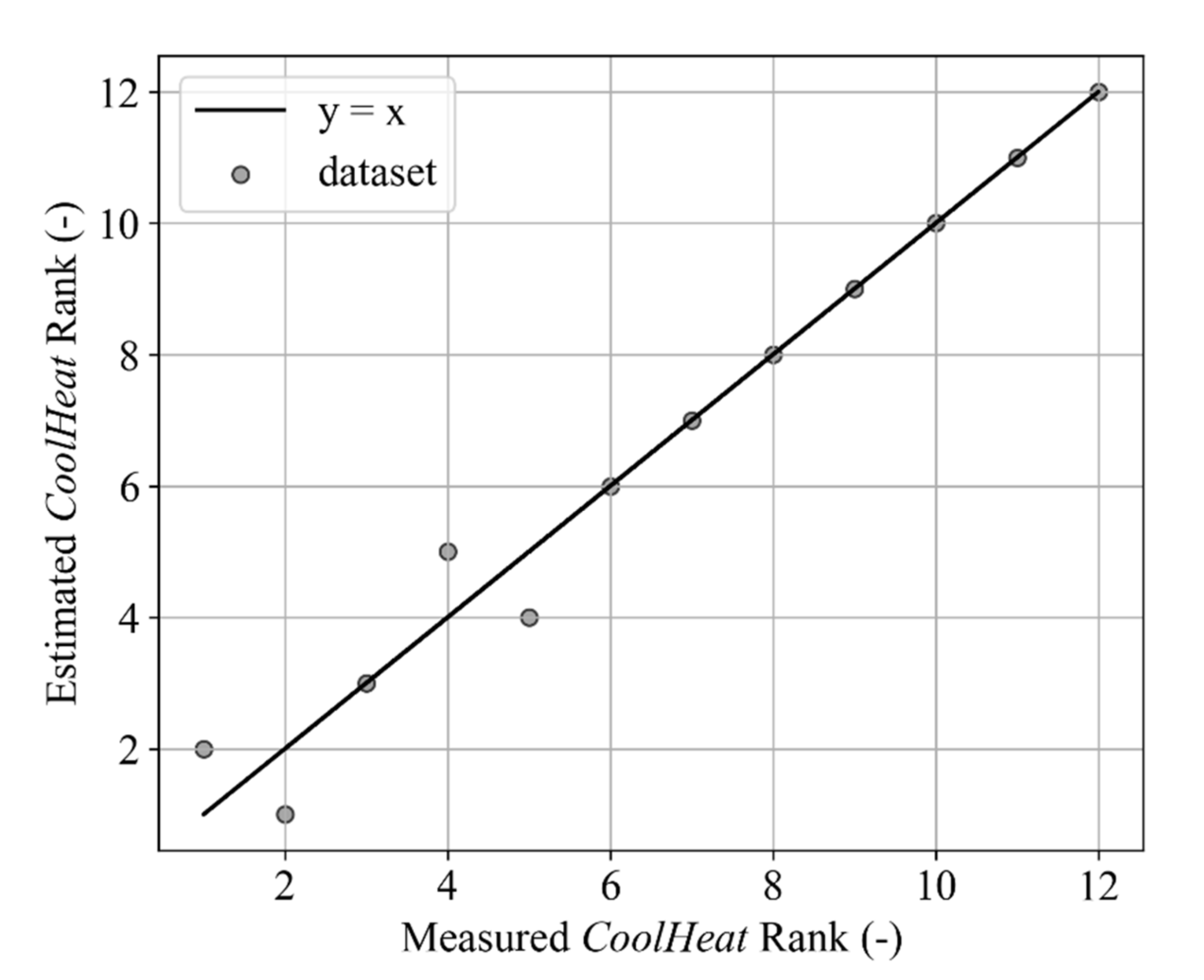
| Index | Segmentation | Total | CoolHeat (Measured) | CoolHeat (Estimated) | |||
|---|---|---|---|---|---|---|---|
| Energy (kWh/m2) | Rank (-) | Energy (kWh/m2) | Rank (-) | Energy (kWh/m2) | Rank (-) | ||
| bldg.#01 | SW | 65.9 | 5 | 41.3 | 8 | 51.7 | 8 |
| Yearly | 79.0 | 3 | 43.1 | 8 | - | - | |
| bldg.#02 | SW | 30.7 | 2 | 17.1 | 4 | 25.5 | 5 |
| Yearly | 40.9 | 1 | 18.9 | 4 | - | - | |
| bldg.#03 | SW | 133.5 | 10 | 104.6 | 12 | 114.1 | 12 |
| Yearly | 157.4 | 10 | 112.7 | 12 | - | - | |
| bldg.#04 | SW | 69.8 | 6 | 59.0 | 10 | 63.5 | 10 |
| Yearly | 80.2 | 5 | 63.8 | 10 | - | - | |
| bldg.#05 | SW | 30.4 | 1 | 10.9 | 2 | 14.3 | 1 |
| Yearly | 58.2 | 2 | 12.8 | 2 | - | - | |
| bldg.#06 | SW | 67.0 | 11 | 28.2 | 7 | 49.7 | 7 |
| Yearly | 90.1 | 11 | 34.4 | 7 | - | - | |
| bldg.#07 | SW | 26.6 | 3 | 5.8 | 1 | 15.3 | 2 |
| Yearly | 40.0 | 4 | 6.2 | 1 | - | - | |
| bldg.#08 | SW | 31.2 | 4 | 17.3 | 5 | 19.1 | 4 |
| Yearly | 43.9 | 6 | 20.5 | 5 | - | - | |
| bldg.#09 | SW | 46.8 | 8 | 24.0 | 6 | 36.7 | 6 |
| Yearly | 67.9 | 9 | 29.2 | 6 | - | - | |
| bldg.#10 | SW | 85.3 | 12 | 71.1 | 11 | 77.7 | 11 |
| Yearly | 102.5 | 12 | 85.0 | 11 | - | - | |
| bldg.#11 | SW | 39.1 | 7 | 12.0 | 3 | 16.9 | 3 |
| Yearly | 61.9 | 7 | 15.0 | 3 | - | - | |
| bldg.#12 | SW | 53.5 | 9 | 42.6 | 9 | 58.2 | 9 |
| Yearly | 66.9 | 8 | 47.2 | 9 | - | - | |
Publisher’s Note: MDPI stays neutral with regard to jurisdictional claims in published maps and institutional affiliations. |
© 2022 by the authors. Licensee MDPI, Basel, Switzerland. This article is an open access article distributed under the terms and conditions of the Creative Commons Attribution (CC BY) license (https://creativecommons.org/licenses/by/4.0/).
Share and Cite
Ahn, K.U.; Kim, D.-W.; Lee, S.-E.; Chae, C.-U.; Cho, H.M. Temporal Segmentation for the Estimation and Benchmarking of Heating and Cooling Energy in Commercial Buildings in Seoul, South Korea. Sustainability 2022, 14, 11095. https://doi.org/10.3390/su141711095
Ahn KU, Kim D-W, Lee S-E, Chae C-U, Cho HM. Temporal Segmentation for the Estimation and Benchmarking of Heating and Cooling Energy in Commercial Buildings in Seoul, South Korea. Sustainability. 2022; 14(17):11095. https://doi.org/10.3390/su141711095
Chicago/Turabian StyleAhn, Ki Uhn, Deuk-Woo Kim, Seung-Eon Lee, Chang-U Chae, and Hyun Mi Cho. 2022. "Temporal Segmentation for the Estimation and Benchmarking of Heating and Cooling Energy in Commercial Buildings in Seoul, South Korea" Sustainability 14, no. 17: 11095. https://doi.org/10.3390/su141711095