Transient Characteristic Analysis of Variable Frequency Speed Regulation of Axial Flow Pump

Abstract

In order to explore the influence of different rotational acceleration on the transient internal and external flow characteristics of the axial flow pump and improve the performance of the pump, numerical simulations and experiments were used to analyze the variable frequency speed regulation characteristics of the axial flow pump. Taking three-dimensional turbulent numerical simulation as the main research method and CFX as the calculation platform, three variable frequency speed regulation methods were used to conduct transient numerical simulation; keep the acceleration constant, increased and decreased; and obtain the real-time pump performance curve and pressure characteristic curve. Uniform acceleration and deceleration with constant acceleration maintained the stable change and good stability of head and shaft power, and the pressure change was the most stable in the process. The acceleration and deceleration with decreasing acceleration ran most smoothly at high speed, and the frequency conversion effect was the best. At the same time, the transition to steady-state operation was also the most stable. The research in this paper can provide reference for the stable operation of variable frequency speed regulation of the axial flow pump.

1. Introduction

Axial flow pumps with larger flow rate and low head [1,2] are widely used in numerous departments of national economics, such as agricultural irrigation, flood control, drainage, water conservancy, etc. [3]. However, in the process of water transportation, the axial flow pump will deviate from the design operating point because of the changes of flow and head caused by many factors [4]. Speed regulation can automatically track the changes in load, adjusting the operating condition of the axial flow pump at any time so that the pump is always in the optimal state [5,6]. At present, frequency conversion technology and a frequency converter are widely used in speed regulation of the pump [7] to save energy in pump stations and realize consumption reduction and economic operation. Frequency speed regulation has become an important development direction of water pump speed regulation [8,9]. Therefore, it is of practical significance to study the transient characteristics of variable frequency speed regulation of axial flow pumps [10].

With the continuous broadening of the application field of axial pumps and the rapid development of intelligent pumps, the influence of unsteady flow and transient external characteristics of axial pumps in the process of speed mutation has attracted the attention of scholars at home and abroad. Tan Jianbo et al. established the energy consumption loss model of the variable frequency pump, which solved the complicated problem of operation variable frequency control and provided theoretical guidance for optimizing the configuration of the variable frequency speed regulation system of pump stations [11,12]. In 2016, Li Na and others pointed out that within the variable speed range, the optimal speed can be obtained by using the golden section to narrow the search interval [13]. Jing Hao et al. used SIMALINK in MATLAB as the simulation platform to realize the simulation calculation of the variable speed and energy-saving adjustment of the parallel pipeline system of the water supply pumping station and constructed the simulation model of the variable speed adjustment of the water supply system [14]. Sha Yi et al. obtained the variation law of the axial flow pump performance curve through type and variable speed external characteristic tests [15]. Zmf A. found that appropriate frequency conversion speed regulation can improve system efficiency and power saving rate, and its frequency conversion characteristics are related to the characteristics of the pipe network and pump [16]. Cimorelli L. et al. compared the energy loss of different pump scheduling technologies and pointed out that the use of variable-speed drives can effectively reduce the operating cost of pump stations [17]. Sun Yuhan et al. analyzed different frequency conversion operation scheduling forms and found that on the premise of meeting water supply demand, frequency conversion operation with parallel scheduling has a better energy-saving effect [18]. Li Xianghui further studied the speed range of variable frequency speed regulation and found that the application range of low-frequency speed regulation is wider [19]. Axial flow pumps have also been used in new fields such as fluidic rolling robots using voltage-driven oscillating liquid [20] and an eccentric actuator driven by stacked electrohydrodynamic pumps [21]. In the process of variable speed, the internal flow field of the axial flow pump are more complex, so there is a lack of systematic and in-depth research on the transient characteristics of an axial flow pump at home and abroad. This paper uses the method of combining numerical simulation and experiment to explore the transient performance of the axial flow pump.

2. Numerical Simulation and Experimental Verification

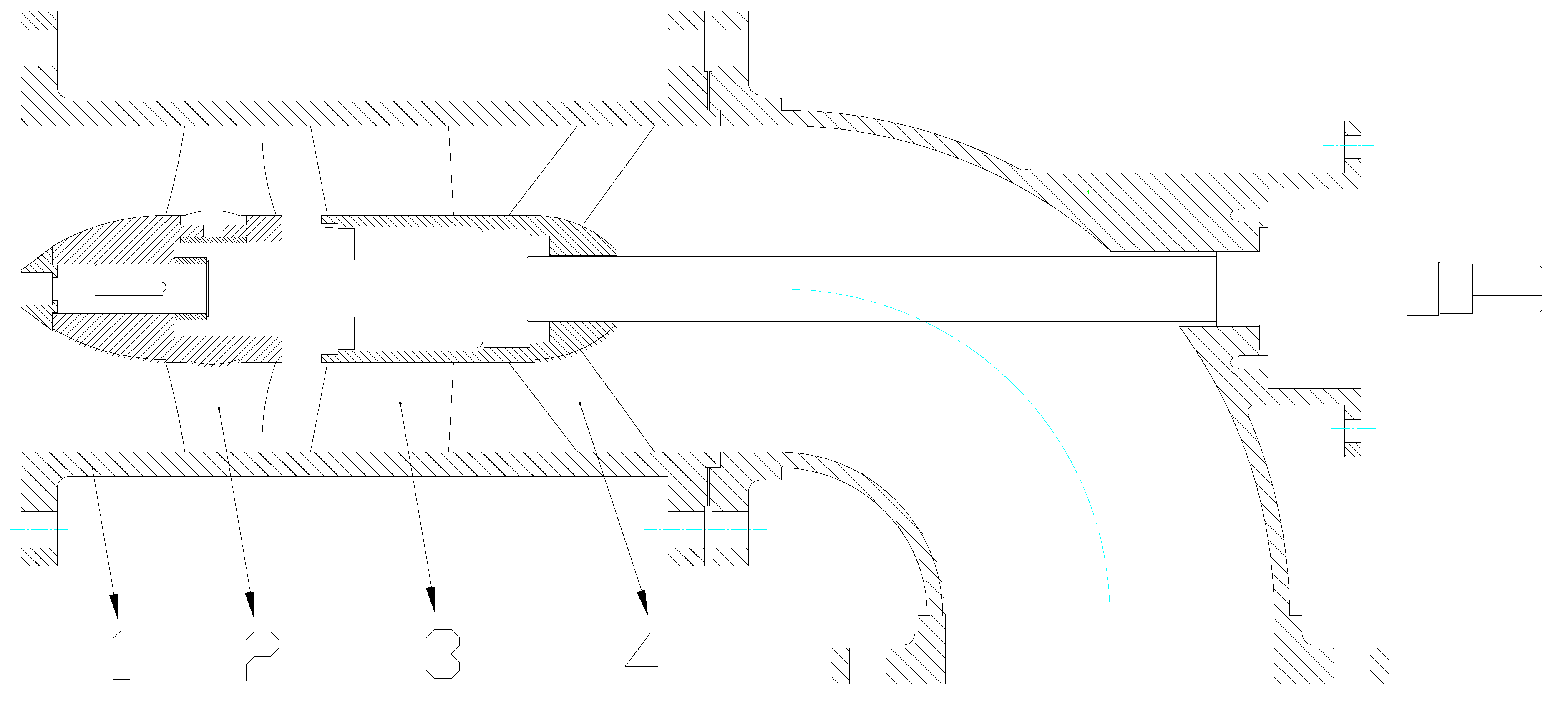
2.1. Simulation Model

Figure 1 shows a 3D geometric of an axial flow pump model with a specific speed $n_s$ = 735 and an impeller diameter of 200mm.

Table 1. The basic design parameters.

Main Parameters	Value
Flow (m3/h)	365
Head (m)	3.02
Number of blades-Zi	3
Number of guide blades-Zs	7
Rated speed-n (r/min)	1450
Impeller inlet diameter-D0 (mm)	200
Impeller outlet diameter-D2 (mm)	250

lists the basic design parameters.

The three-dimensional physical model of the axial flow pump is shown in Figure 2. The main hydraulic components such as the impeller and guide vane are created by SolidWorks 2021.

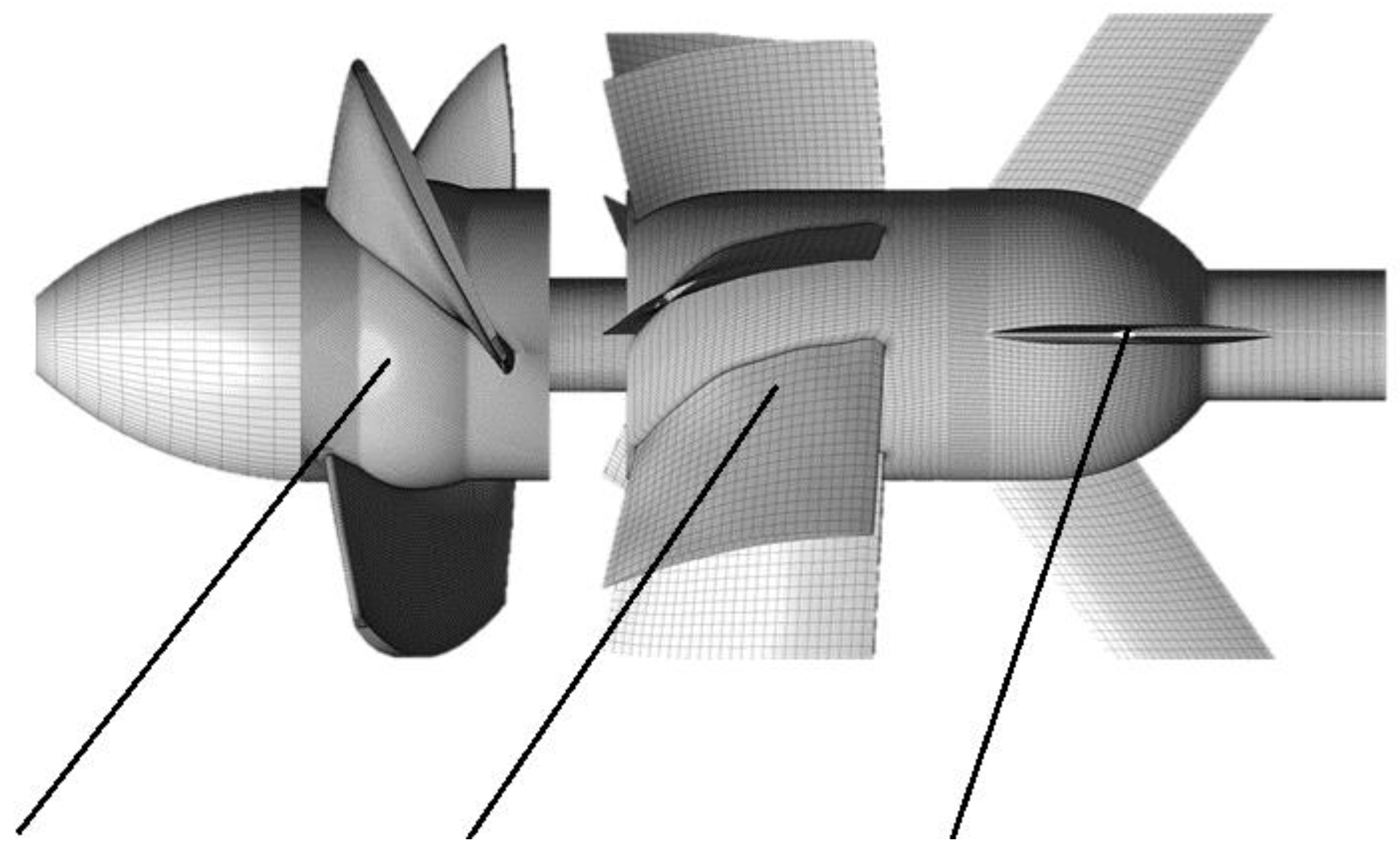
2.2. Meshing and Validation of Mesh Independence

The pump model is meshed by Pointwise. The clearance between the impeller and the impeller chamber adopts mixed mesh because it is relatively small. At the same time, the inlet, outlet, and volute adopt the hexahedron structure mesh with better convergence. Adjust the number of grid nodes on each topology line to make the computing domain mesh change evenly and encrypt the mesh on the impeller and interface.

Under the design operational condition, the numerical simulation results remained unchanged when the number of grids reached 10.09 million, taking the rated head as the index, which can verify the independence of the mesh. The mesh division of main flow components is shown in Figure 3.

2.3. Boundary Conditions

CFX software is used for numerical simulation based on the continuity equation and Reynolds average N-S equation. The impeller is set as a rotating domain, the rest is a static domain, and the interface of static and dynamic is set as a frozen rotor. Choose 25 ℃ water as a medium and standardize the k-ε model as a computational model. The wall is smooth without slip. The pump’s internal reference pressure is set to one standard atmospheric pressure. Inlet and outlet parameters are set according to the actual situation of the pump station. Set convergence accuracy as 10⁻⁴. The inlet is set as the total pressure inlet, the pressure value is set as zero, and the reference pressure is set as 50kPa. The outlet is set as the mass flow outlet, and the external characteristic curve of the pump can be obtained by setting different mass flows.

2.4. Experimental Investigation

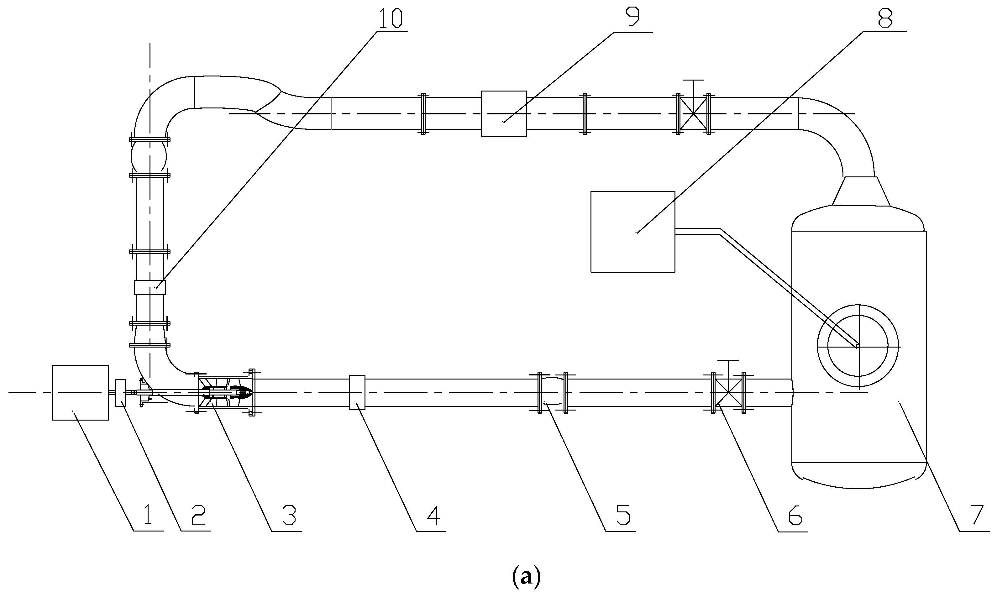
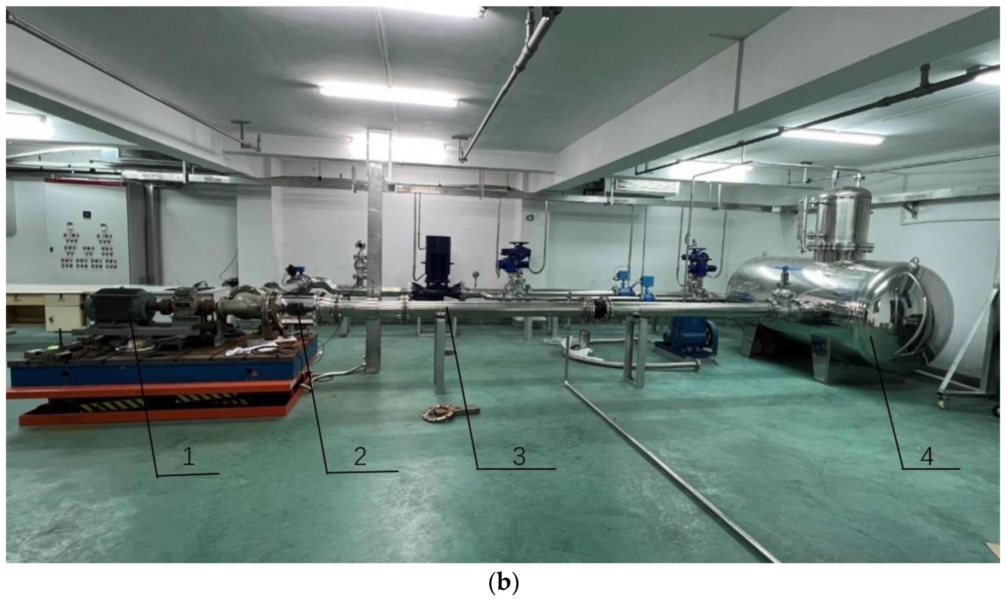
2.4.1. Experimental Apparatus

The steady-state external characteristic test and PIV test are carried out for the model pump in this paper, which was completed in the Key Laboratory of Pump and System Energy Saving Technology for Petroleum and Chemical Industry, School of Mechanical Engineering, Nantong University. Affected by the data acquisition response rate of the test bench, this paper mainly tests the basic performance of the test pump under different operating conditions to verify the accuracy of the numerical simulation results. Figure 4 shows a schematic diagram and physical figure of the model pump test bench.

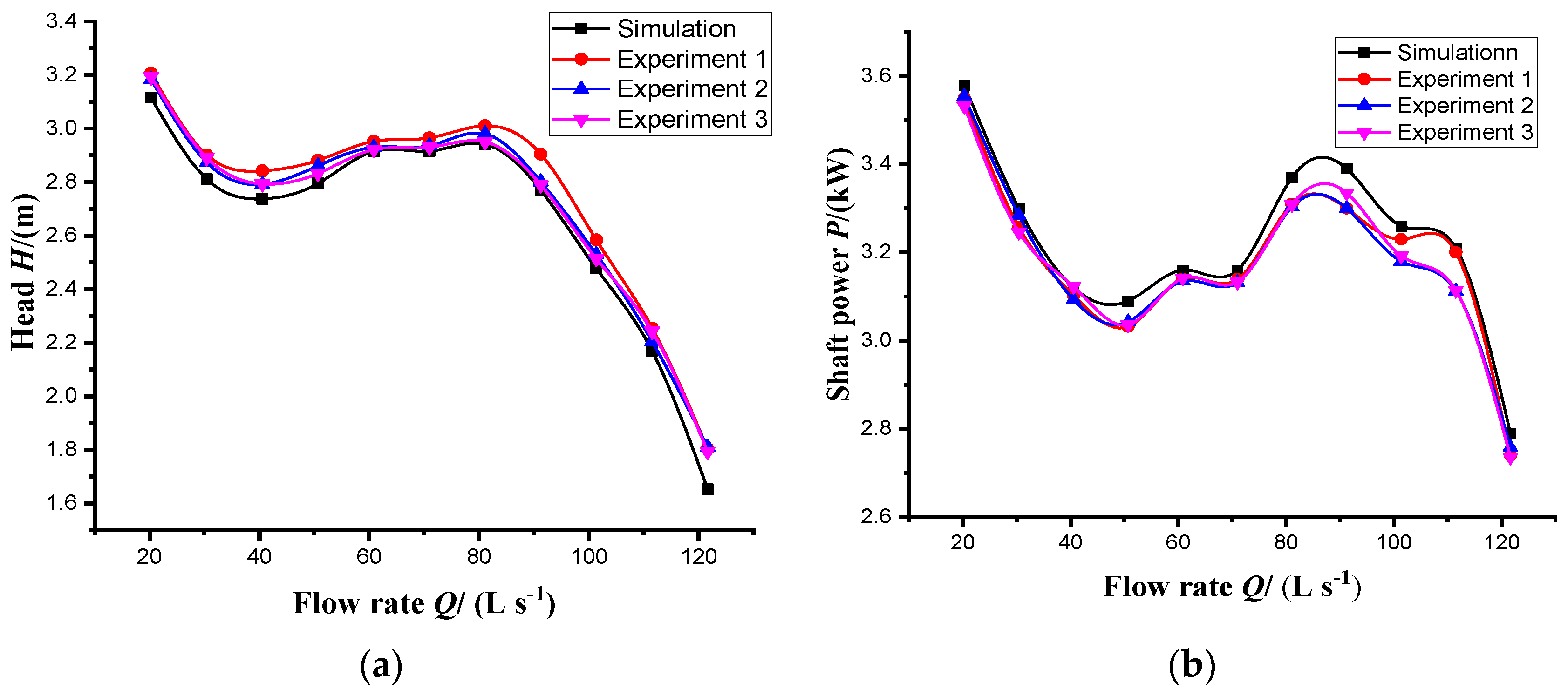
2.4.2. Steady-State Pump Performance Test

According to the data obtained from the steady-state pump performance test and the pump performance obtained from numerical simulation, the pump performance curve is drawn as shown in Figure 5. It can be found that the curves of the three test values roughly coincide, but due to the influence of the booster pump, the test values of head and efficiency are generally higher than the simulated values, and the shaft power is slightly lower than the simulated values. However, the overall variation trend with flow conditions is consistent with the numerical simulation value, which ensures the accuracy of numerical simulation.

3. Analysis of Numerical Simulation Results

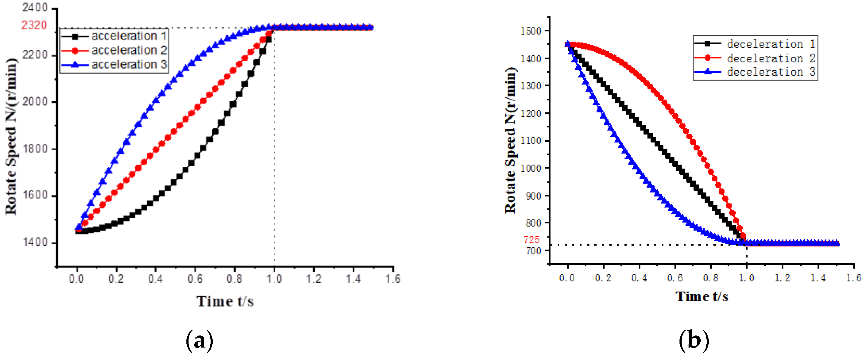
3.1. Transient Numerical Simulation of Variable Frequency Speed Regulation

Take the results of steady calculation as the initial value. Unsteady numerical simulation was used to analyze the flow field distribution and pressure pulsation in the process of frequency conversion. This paper uses CEL expression to simulate different forms of frequency conversion methods. This study selects three forms of speed change. In order to highlight the comparison of pump performance under different rotational speeds, the increase in rotational speed was set at more than 50% of the rated speed, and the decrease in speed was set at half of the original rated speed. Figure 6 is the variation curve of rotational speed with time drawn according to the expression.

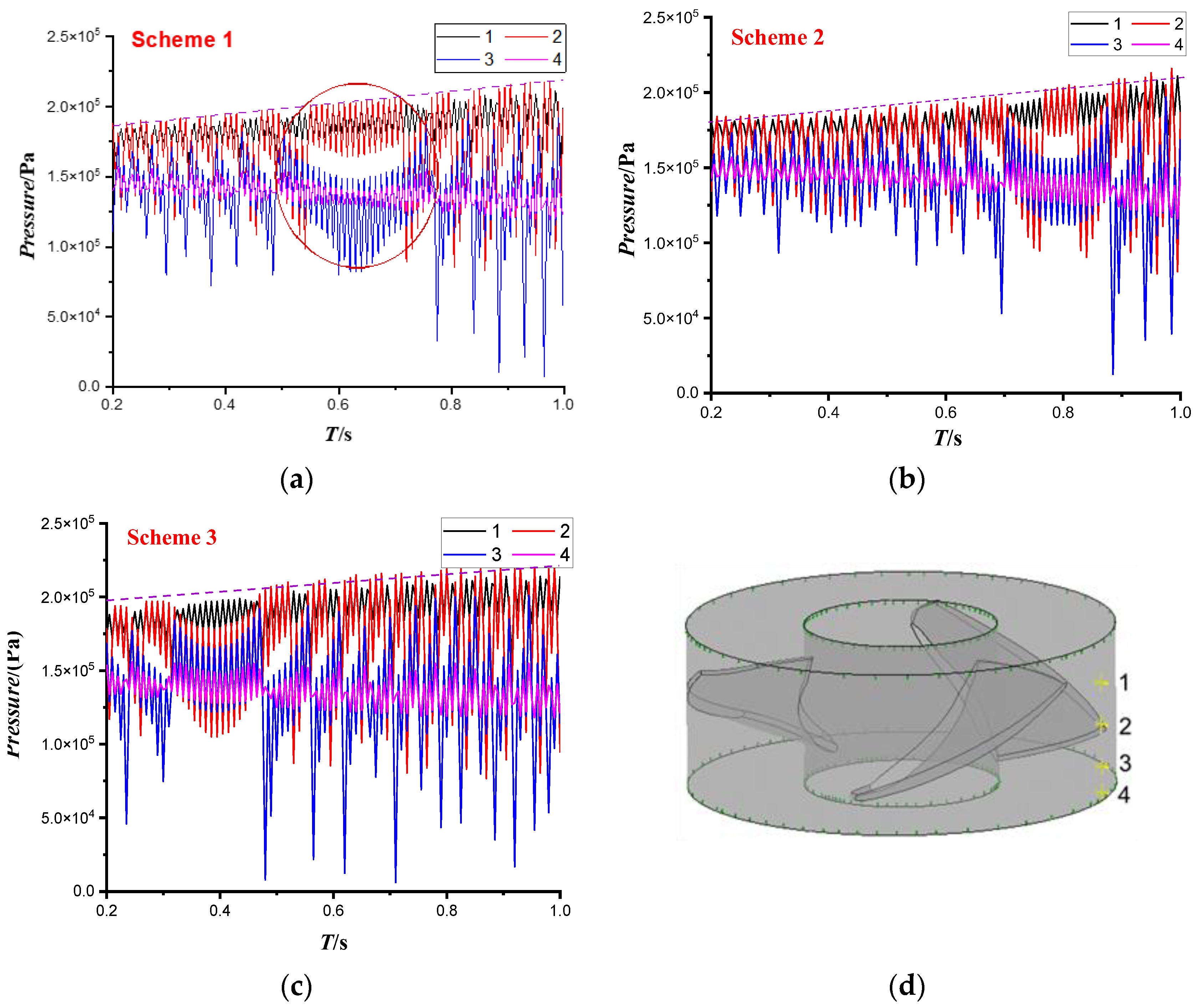
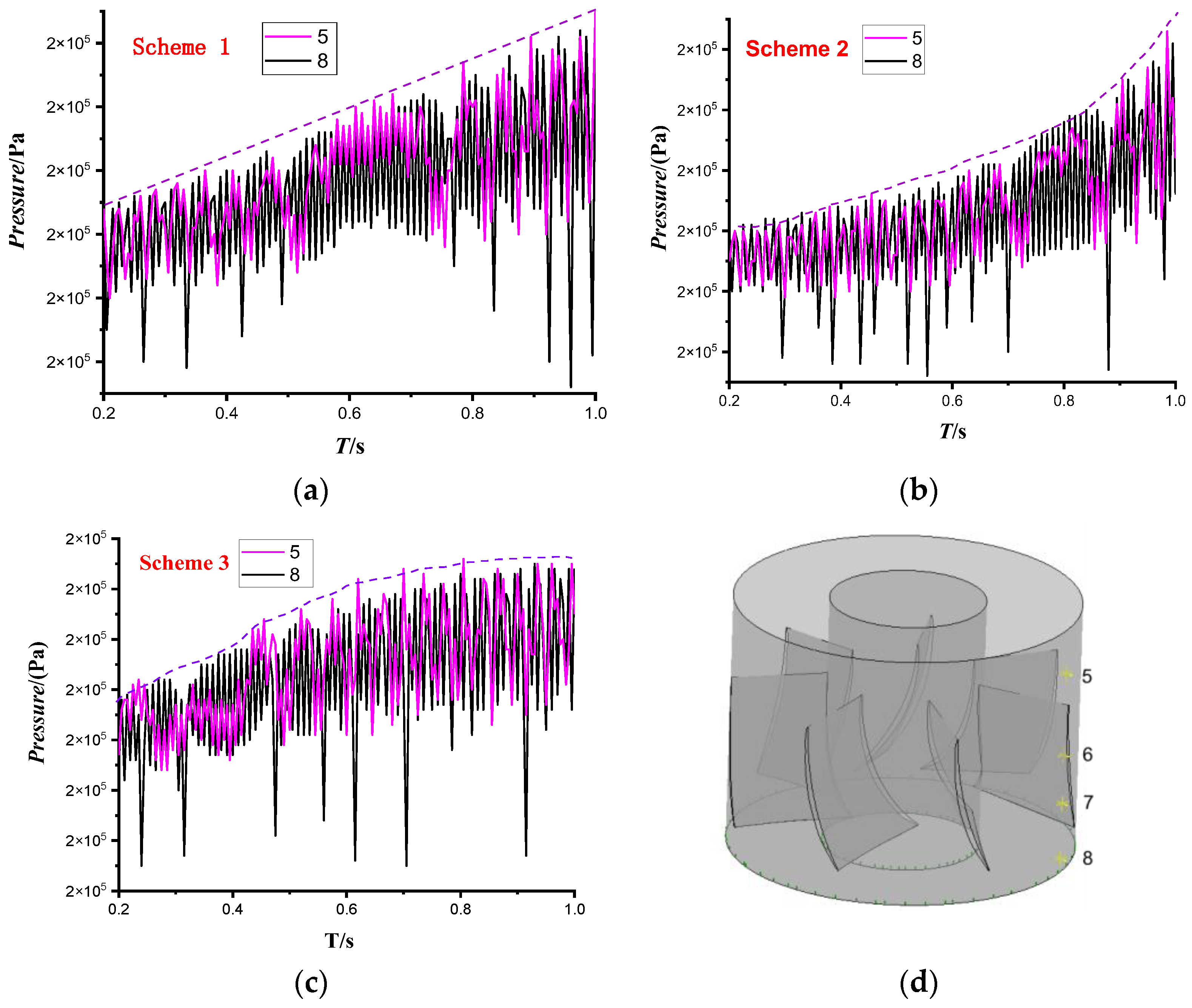
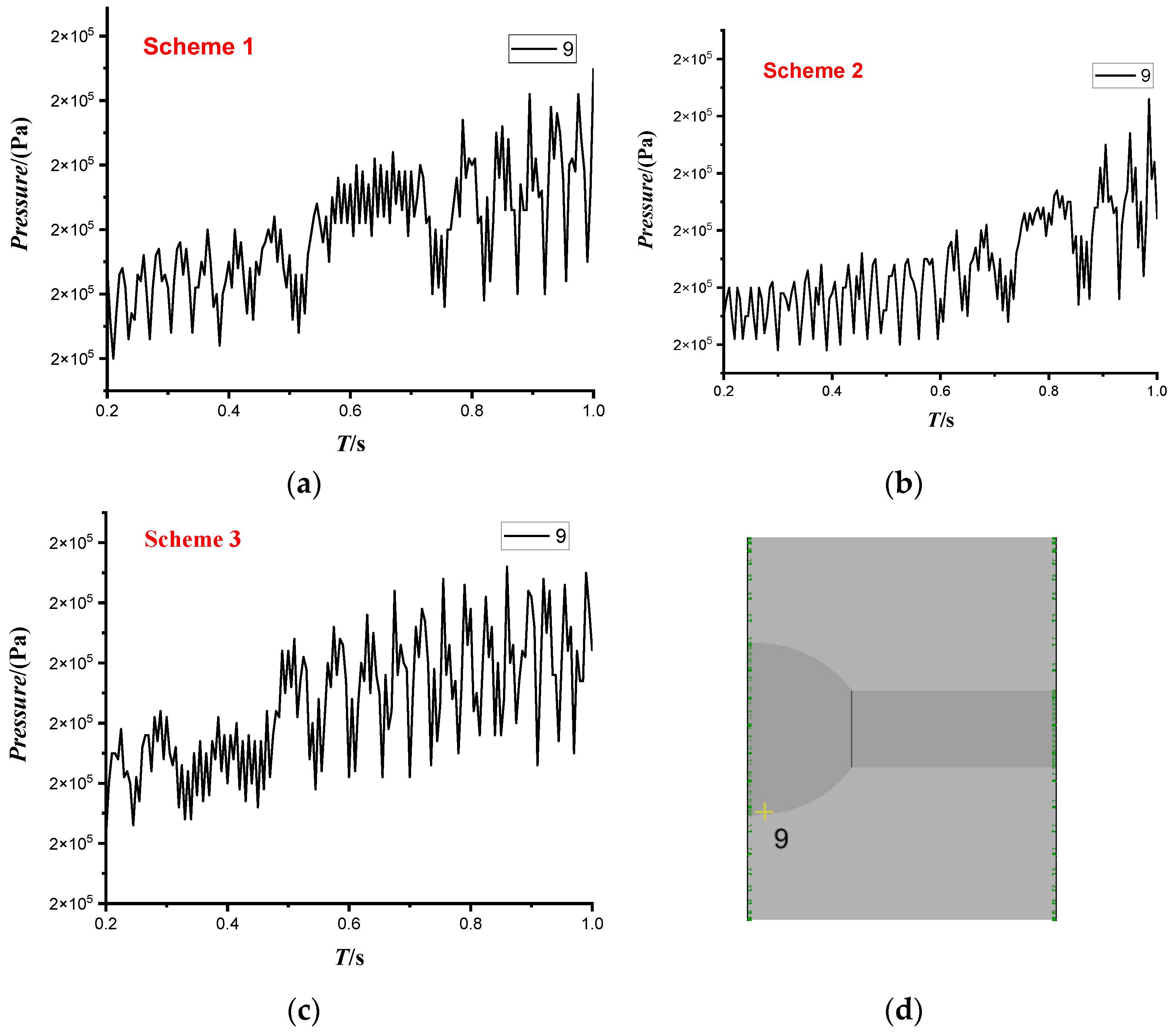
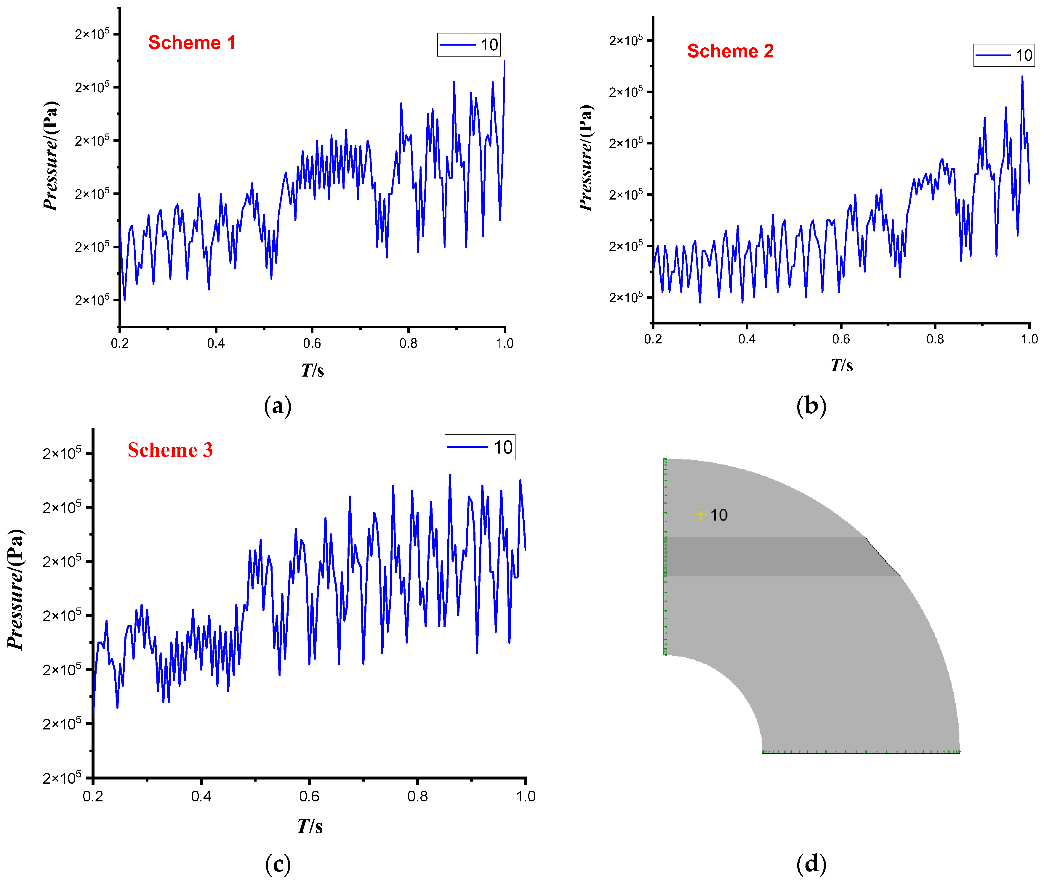
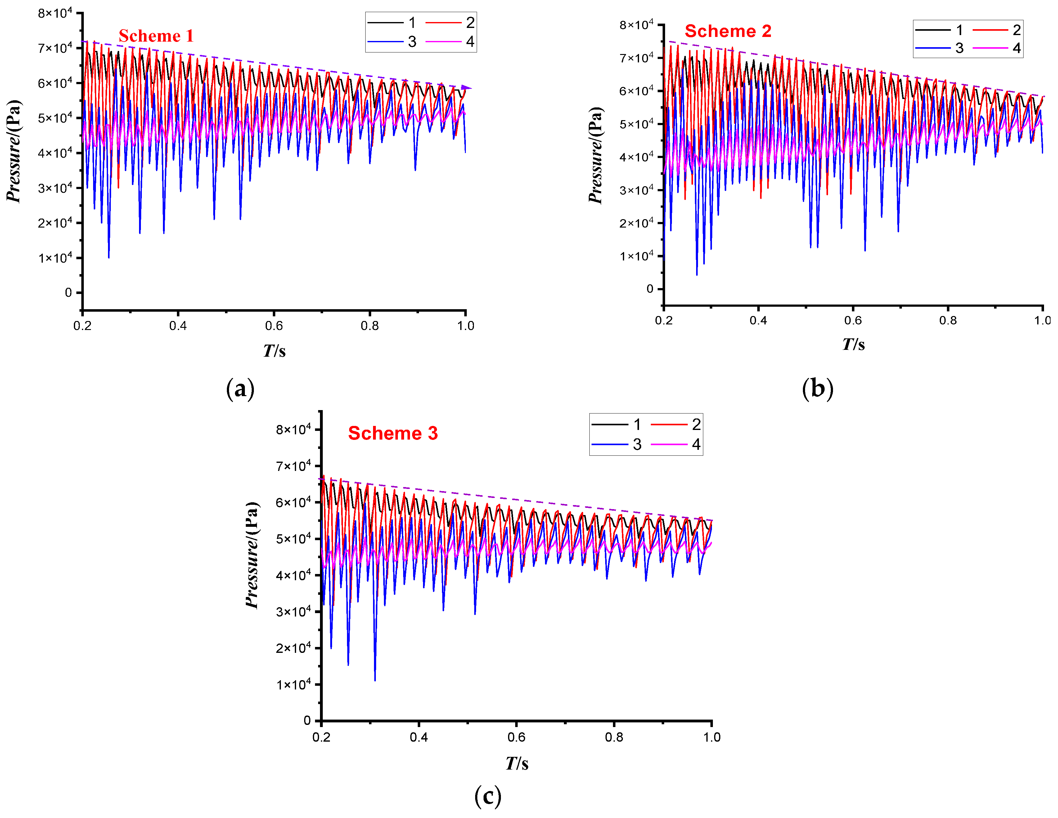
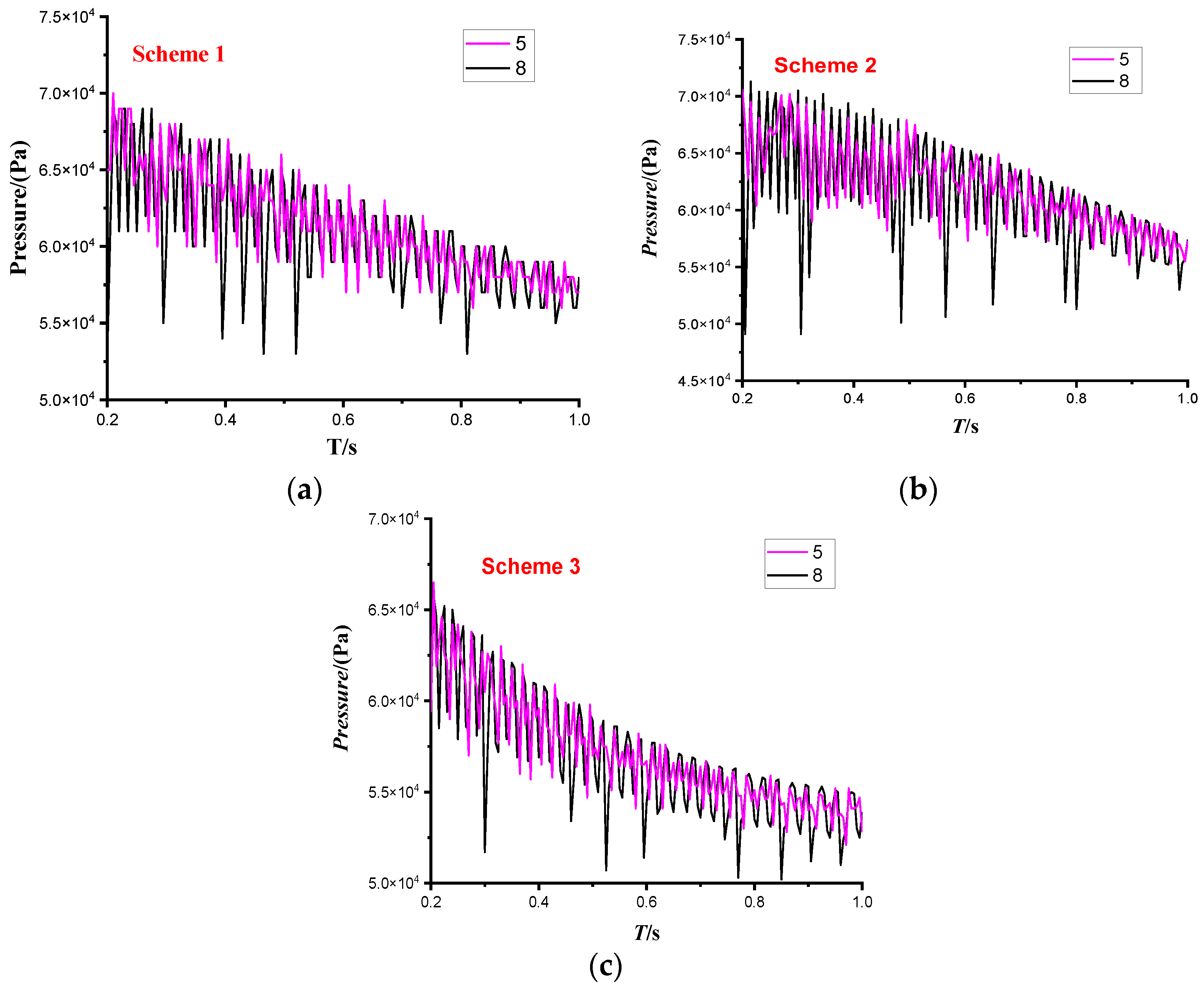
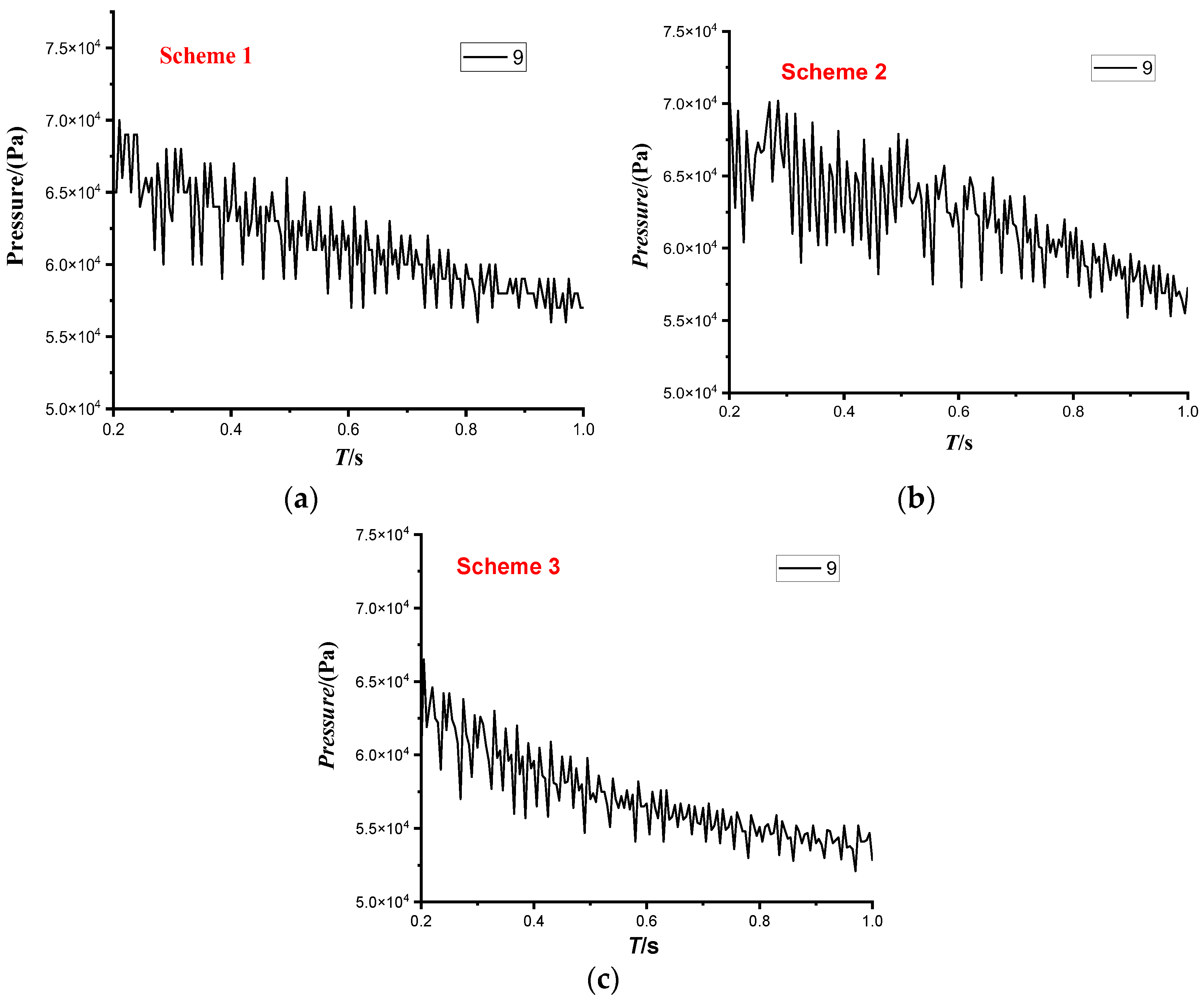
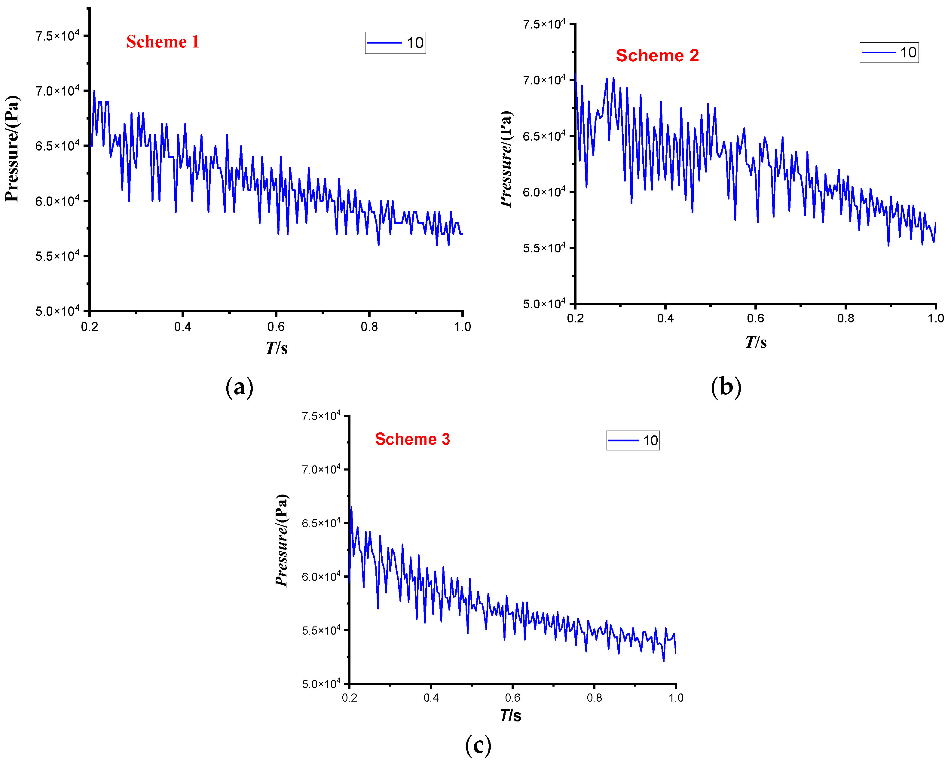
3.1.1. Pressure Distribution

In the process of acceleration, the inlet pressure is taken as 150 kPa. Monitoring points are impeller inlet 4, impeller middle 2, 3, impeller outlet 1, guide vane inlet 8, guide vane middle 6, 7, guide vane outlet 5, support plate middle 9, and elbow middle 10. At the beginning of the operation of the pump, the pressure changes are quite chaotic, so the pressure changes are taken from 0.2 s to 1.0 s, as shown in Figure 7, Figure 8, Figure 9 and Figure 10. By comprehensively observing the changes of all monitoring points in the impeller, we found that the changing trend at 0.5 s of scheme 1, 0.7 s of scheme 2, and 0.3 s of scheme 3 is different from the surrounding. The acceleration values of the three schemes at the moment when the pressure appears are calculated, which are all about 870, indicating that the acceleration will affect the local distribution of the pressure in the pump. By comparing the pressure changes of three schemes, the pressure growth of scheme 1 is relatively stable, while that of scheme 3 changes slowly over time.

In order to facilitate observation, only point 8 at the inlet of the guide vane and point 5 at the outlet of the guide vane are taken. As shown in Figure 8, the pressure fluctuation in the guide vane is significantly smaller than that in the impeller. The overall growth trend of the pressure at the outlet of the guide vane is the same as that of the rotational speed of different schemes, as indicated by the dotted line in the figure. The pressure changes at the guide vane, support plate, and elbow of different schemes are comprehensively compared. Scheme 3 shows the largest pressure fluctuation and mean value, but the change is relatively stable over time, and the flow in the guide vane and the flowing parts behind tend to be stable in the late acceleration period. On the contrary, in scheme 2, the difference between the maximum value and the minimum value is small, but the pressure value keeps increasing with the changes of speed, and so does the pressure range. The guide vane is subjected to a small continuous impact of high and low pressure, but with the constant increase in pressure value, it is easy to lead to the vibration of the guide vane. Overall consideration, acceleration scheme 3 has the most stable pressure change and the best acceleration performance.

In the deceleration scheme, the inlet pressure is 50 kPa. Figure 11, Figure 12, Figure 13 and Figure 14 show the changes in pressure at each monitoring point over time in different deceleration schemes. In the figure, the pressure difference at the impeller gradually decreases with time, among which the pressure changes the most in deceleration scheme 2, whose maximum pressure is much higher than that in other deceleration schemes. The dynamic change of pressure in deceleration scheme 1 is stable. In scheme 3, the pressure changes dramatically at the beginning. After the deceleration reaches 0.6 s, the pressure at all monitoring points does not change. After 0.8 s, the periodicity is obvious. Scheme 3 is more stable when the deceleration is complete. According to the changes of three schemes in the impeller, the pressure amplitude is generally large at the beginning of deceleration, but the transition of schemes 1 and 3 is better than that of scheme 2. Further observation of the pressure distribution at the guide vane, support plate, and elbow shows that the pressure distribution at static parts is roughly the same, and the pressure decrease trend is the same as the changing trend of the velocity change scheme. By comparing the pressure changes of static components in each scheme, the pressure of scheme 3 is smaller than that of the other two schemes. On the other hand, it can be established that scheme 1 and scheme 3 have the least pressure fluctuation. It can be concluded that in the process of deceleration, from the perspective of pressure distribution, the overall stability of scheme 1 and scheme 3 is better.

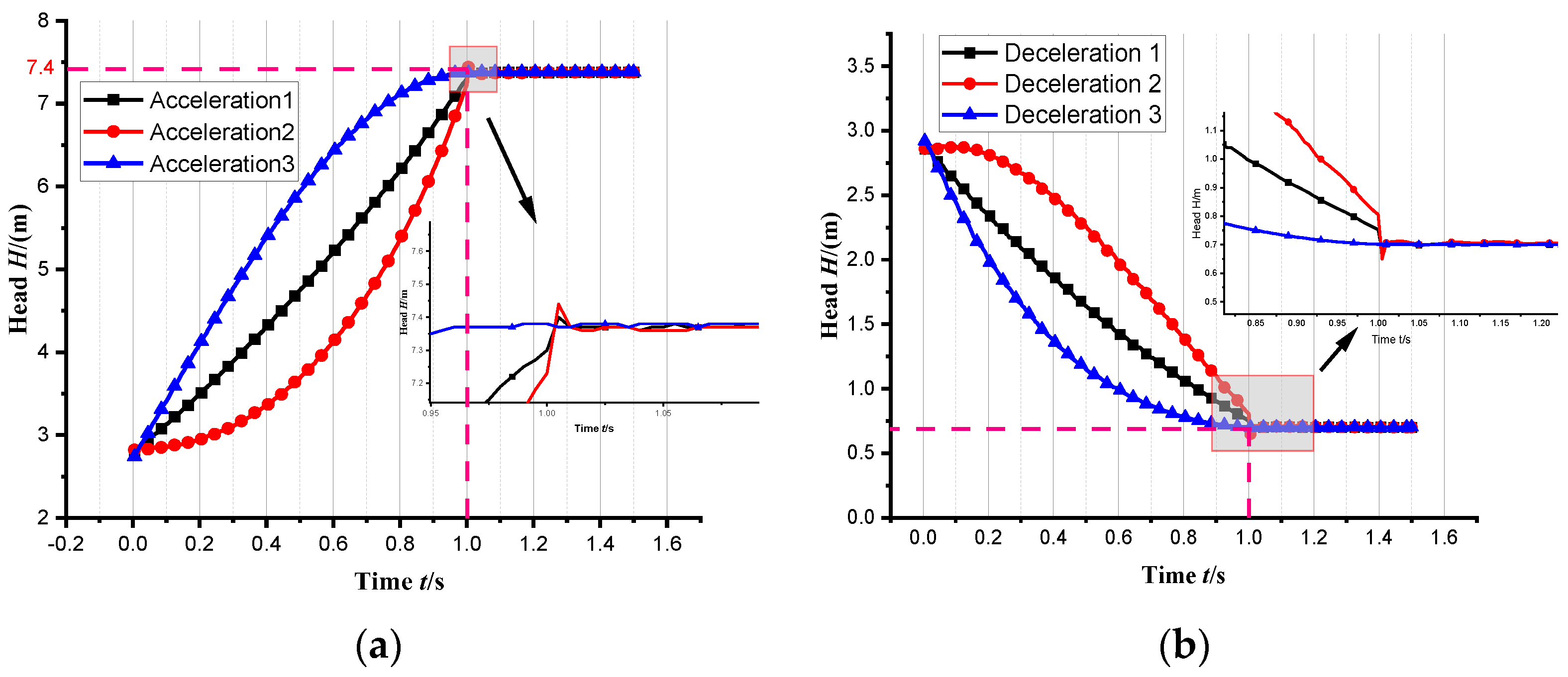
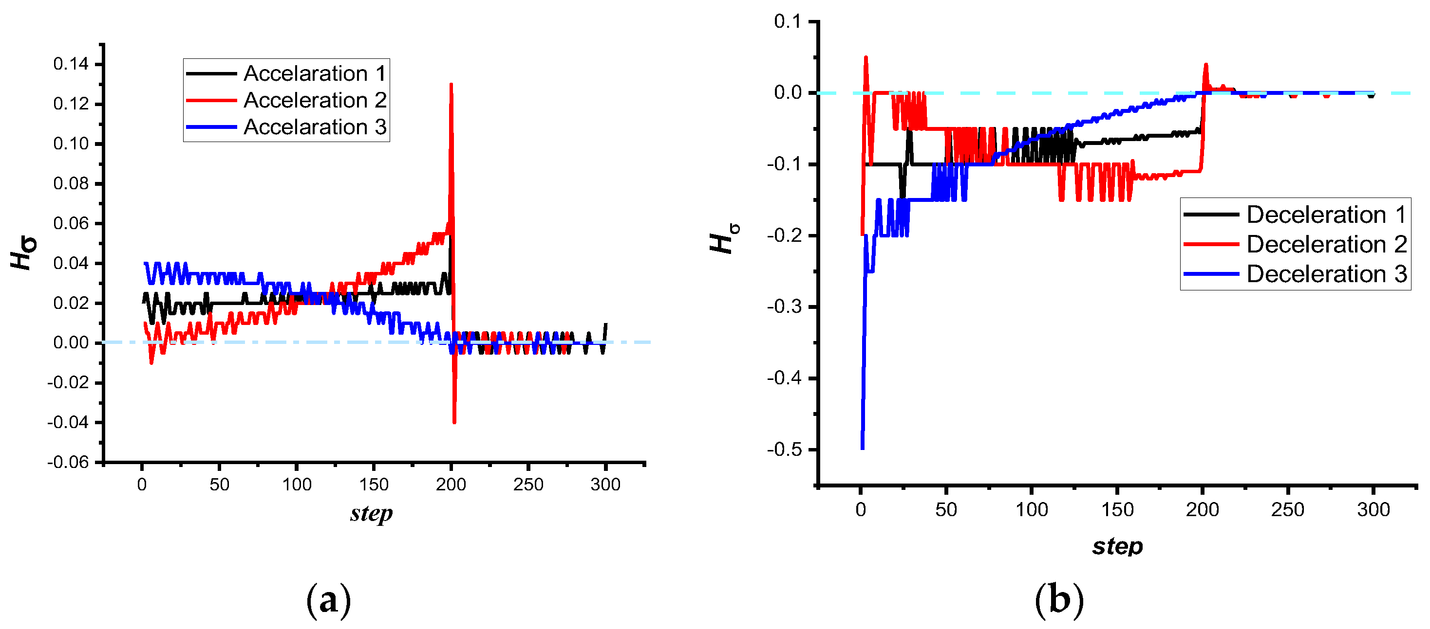
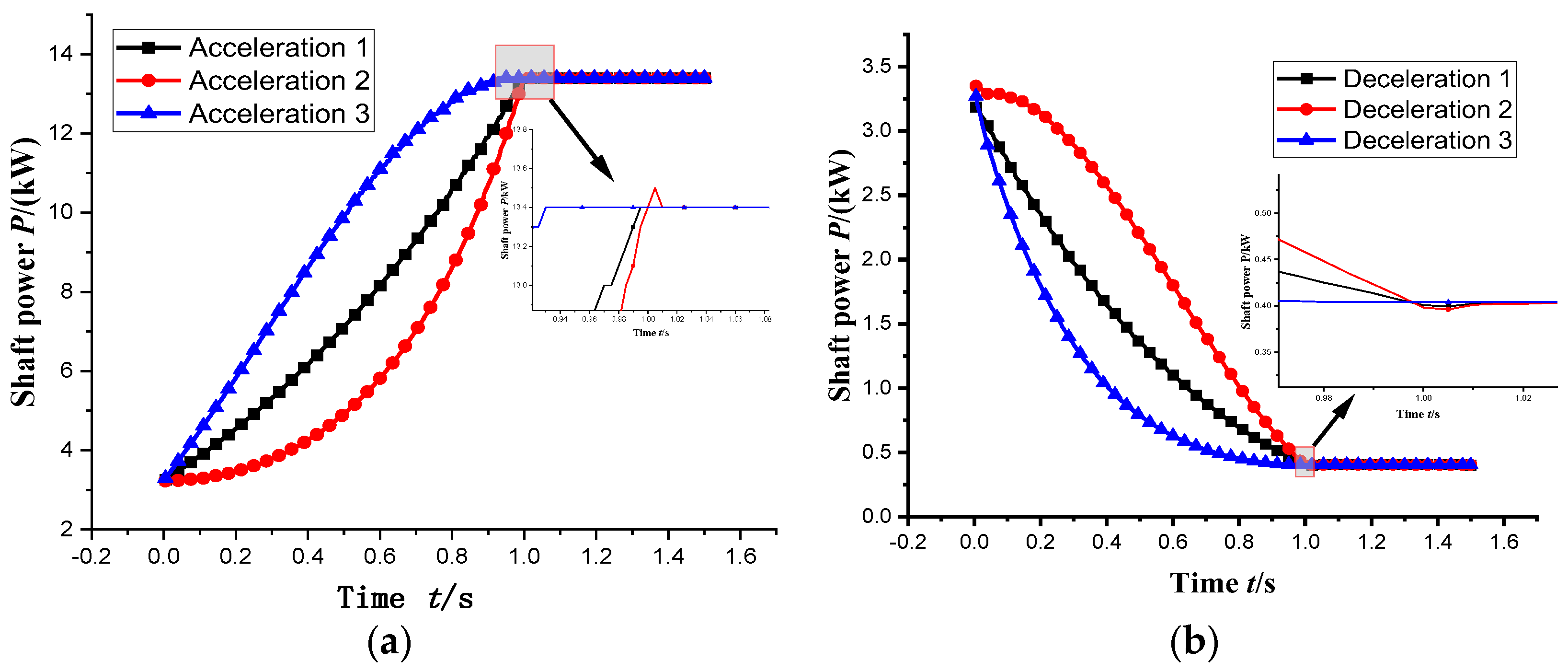
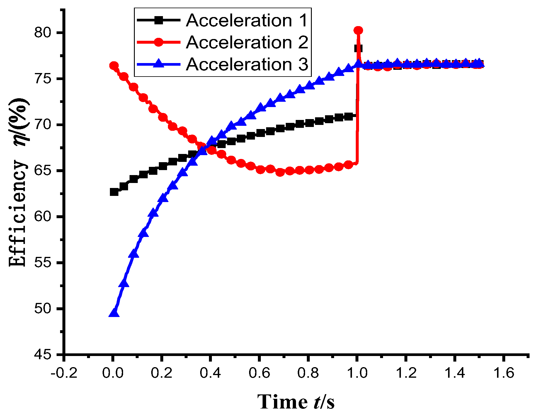
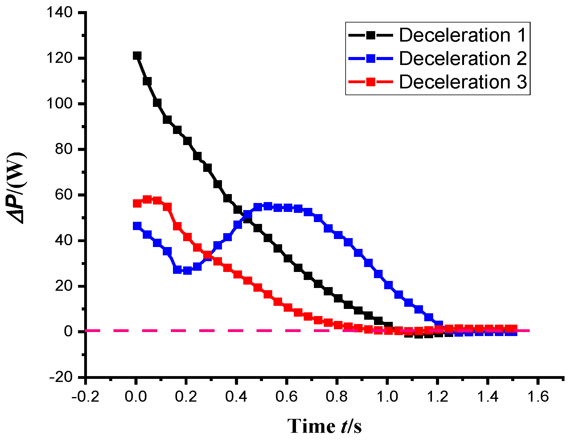
3.1.2. Transient Pump Performance under Variable Frequency Speed Regulation

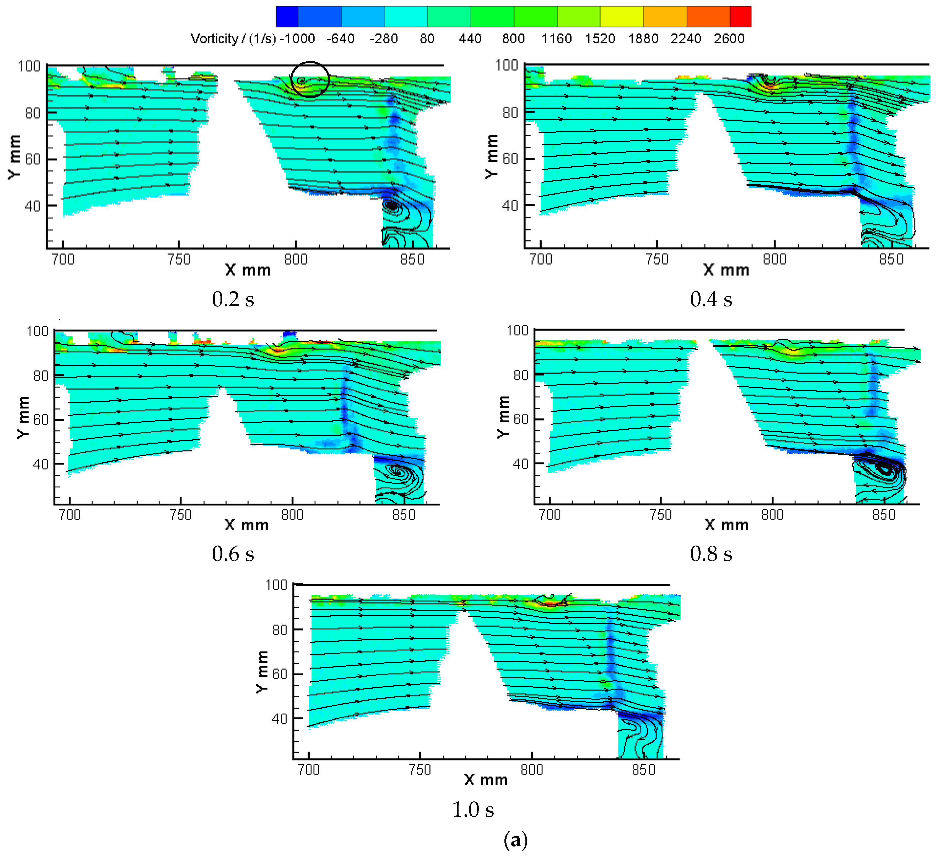
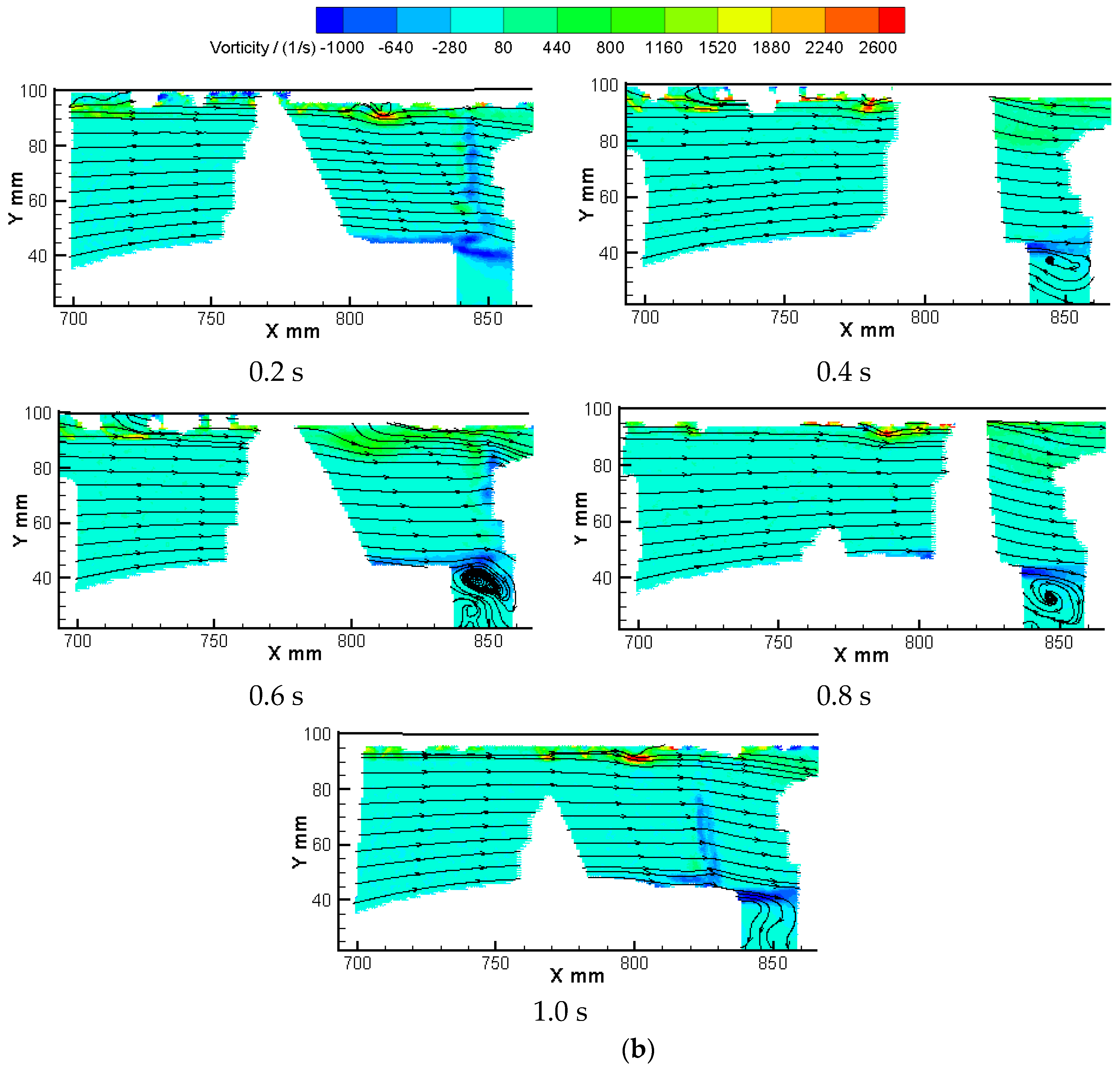
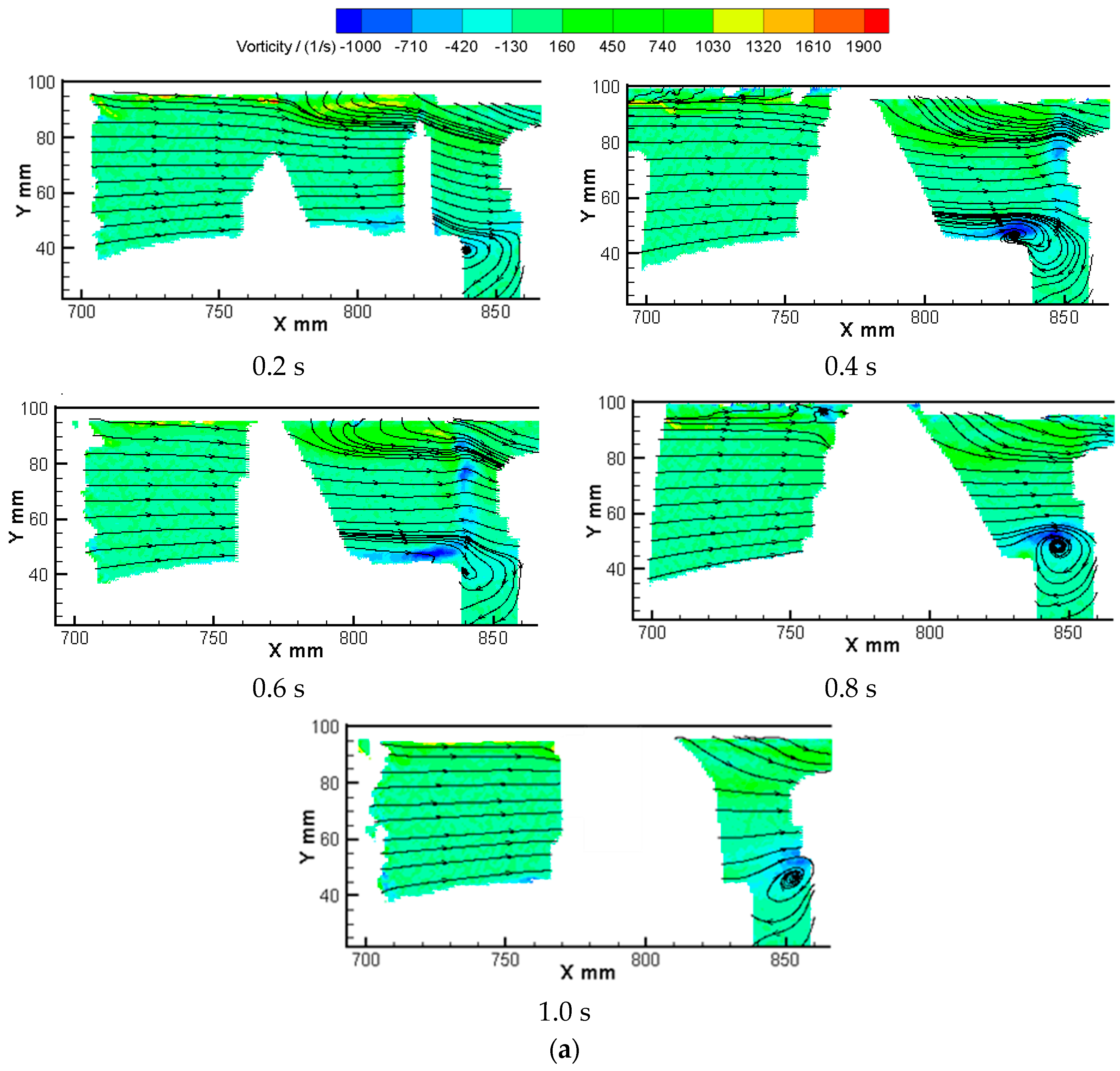
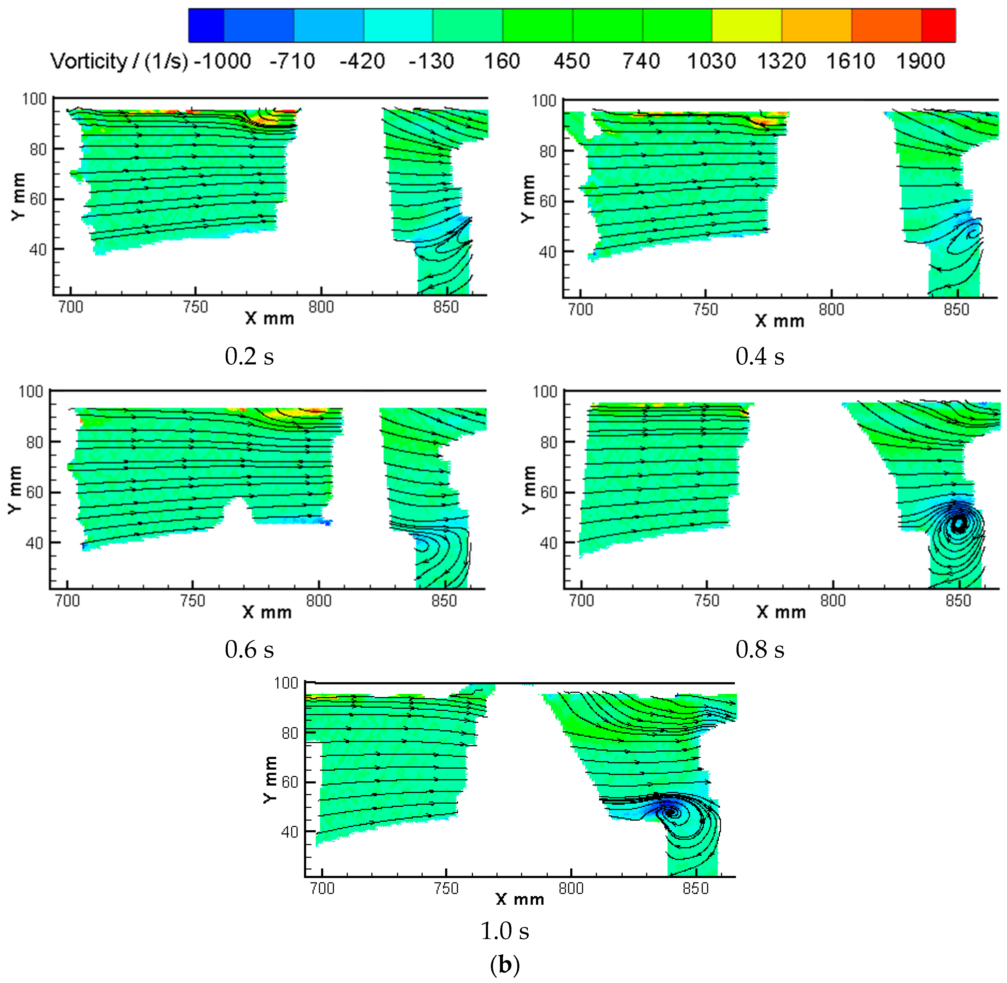
Based on the above three acceleration and deceleration schemes, take the design working condition as the starting point to accelerate and decelerate, draw the real-time pump performance curves of various frequency conversion schemes, and explore the most suitable frequency conversion scheme. After setting inlet pressure, variable speed, and corresponding flow, the real-time head change curve is shown in Figure 15. Figure 15a shows the head distribution diagram of three different acceleration schemes with time. It can be seen from the diagram that the change of head over time is roughly the same as the above speed variation trend, but it does not significantly exceed the established head. Zoom in at the 1s fold point, as shown in the lower right corner, and it can be found that the acceleration scheme with decreasing acceleration approaches the target headfirst, and the uniform acceleration scheme comes second. In contrast, by comparing the head fluctuation of the three after speed regulation, it is found that the acceleration scheme with decreasing acceleration can better maintain the stability of the head and have a more efficient speed regulation performance after speed change.

Figure 15b shows the corresponding three deceleration schemes. Similar to the acceleration schemes, the three deceleration schemes have the same change trend and speed change, and scheme 3 has a better deceleration effect. By observing the enlarged figure, it can be found that after completing the deceleration process, the head of the three schemes shows a cliff-like phenomenon, among which the transition of the head of scheme 3 is the most stable, while the change of head of scheme 2 is the most drastic. It can be explained that the variable speed process with decreasing acceleration value, whether accelerating or decelerating, has an efficient variable speed effect, and it can still maintain good stability after the variable speed is completed.

In order to show the stability of head with speed change more intuitively, the head change rate is introduced. Draw the change curve of head change rate with time step, as shown in Figure 16. It is further explained that the acceleration scheme 3 can ensure the steady growth of the pump head in the acceleration process, that is, to ensure the steady growth of the pressure at the same time that the speed increases. Figure 16b shows the curve of head change rate under deceleration. The value of head change rate under deceleration is relatively large, and the curve of head change rate is distributed in stages and steps. In scheme 1, the head fluctuation is small, and after the deceleration is completed, the head change rate will have a small mutation. It shows that the uniform deceleration scheme is better from the head stability alone.

The change of shaft power with time is shown in Figure 17. The changing trend of shaft power is roughly similar to that of the head. During the acceleration process, the overall distribution of the shaft power curve in scheme 3 is relatively stable. On the contrary, in scheme 2, the shaft power increases steadily at the beginning of acceleration, but after the acceleration, it is found that scheme 2 has an obvious “hump” turning area and obvious impact by observing the enlarged figure at the lower right corner. At this time, the speed is large, and the pump will also be impacted by the acceleration, so acceleration scheme 3 is better than acceleration scheme 2. Similarly, in the deceleration scheme, the shaft power of scheme 3 decreases the fastest, and after the deceleration is completed, it can smoothly transition to a stable state, which has a good deceleration effect.

In the process of acceleration and deceleration, the efficiency will also change with time. Figure 18 shows the efficiency change in the transient acceleration process of the pump.

In the figure, the transient efficiency of the pump is generally low due to inertia during acceleration. Then it increases with time, and the efficiency change of scheme 1 is relatively stable, which shows that maintaining steady acceleration can make the pump have higher operating efficiency in the acceleration process. However, due to the short acceleration process, the impact on the overall operational efficiency of the pump is limited.

In the deceleration state, the shaft power difference is used for efficiency comparison, as shown in Equation (1):

$$\Delta P=P_{st}-P_{tr}$$

(1)

where $P_{st}$ is the steady-state shaft power; $P_{tr}$ is the transient shaft power.

Figure 19 is the relationship curve of efficiency change with time at different speeds drawn according to the above formula. Among the three deceleration schemes, the uniform deceleration scheme has the best energy-saving effect. The deceleration scheme with decreasing acceleration has the best running stability despite of low energy-saving effect.

3.2. PIV Experiment

Through numerical simulation calculation, it is understood that the scheme of uniform speed change and the scheme of decreasing acceleration have better frequency conversion speed regulation performance for the axial flow pump. Therefore, this PIV test is mainly to compare and verify the two schemes and analyze the transient characteristics of the flow field in the axial flow pump. A total of 50 tracer particle images are taken by the camera every second, and 1 particle image is taken from every 10 images for analysis. The streamline image is the velocity vector image, and the cloud image is the vorticity image of the current flow field. Figure 20 and Figure 21 respectively show the flow field distribution of different schemes.

Figure 20 shows the distribution of vorticity cloud diagram of the two acceleration schemes. It can be observed in the figure that obvious reflux phenomenon occurs in the lower right side of each flow field diagram, and its position is just at the junction between the impeller hub and guide blade. Due to the effect of dynamic and static interference, the flow field changes there will be relatively disordered. In the early stage of acceleration, as shown in the circle in the figure, a slight vortex begins to appear on the upper side of the working face of the impeller, and the streamline is also dense, which was caused by the disturbance of the flow around the blade edge of the working face. As the vortex guide blade moves, an obvious blue area can be found at its rear side. At this time, the reverse vortex and the forward vortex begin to contact and offset, and the flow field tends to be stable. As the speed increases, an obvious vortex phenomenon also begins to appear on the back of the blade, mainly because the pipe diameter is not equal to the diameter, and the constant change of velocity makes the flow field near the wall of the front section of the impeller appear to have larger forward vorticity. The reflux phenomenon at the outlet of the right lower impeller becomes more serious, while there is no obvious fluctuation in the streamline at other positions. There is no obvious difference in the flow field changes of different schemes, but in the position where the vortex appears, the vortex changes irregularly in the acceleration scheme with the decreasing acceleration. Therefore, different acceleration schemes in Figure 20 have less impact on the flow field of the entire impeller area. The test pump is suitable for frequency conversion acceleration operation, and the higher efficiency scheme 3 can be used to achieve high-efficiency variable speed.

Figure 21 shows that the vorticity distribution of pump deceleration schemes is opposite to that of acceleration schemes. At the early stage of deceleration, the positive vorticity near the wall surface is obvious. With the decrease in velocity, the positive vorticity decreases, and the streamlined distortion disappears gradually. At 1s, after the deceleration is completed, the vortex structure is invisible, and the streamline begins to flatten.

It can be concluded that different frequency conversion acceleration schemes have little influence on the flow field change. The flow field of a uniform deceleration scheme is more stable than that of a constant acceleration scheme. It is consistent with the numerical simulation.

4. Conclusions

This paper takes a small axial flow pump as the research object; studies the internal flow field, external characteristics, and pressure distribution of the axial flow pump under different frequency conversion and speed regulation forms; and verifies the accuracy of the numerical simulation results through experimental methods. The main research work and conclusions are as follows:

(1)

The variable speed form of the axial flow pump can choose scheme 1 (uniform acceleration and deceleration) or scheme 3 (acceleration and deceleration with decreasing acceleration), wherein scheme 1 can maintain the stable change of head and shaft power and better energy saving effect; the biggest advantage of scheme 3 is that it can reach the predetermined head in advance and can transition to a stable operation state when the speed change is completed. When it is necessary to speed up to a higher speed, scheme 3 is the best choice.

(2)

Different frequency conversion speed regulation methods will affect the local distribution of pressure in the pump. The acceleration scheme with continuously decreasing acceleration has the most stable pressure change and the best acceleration performance. The deceleration scheme with continuously decreasing acceleration has the smallest pressure, small fluctuation, and good stability.

(3)

The change of velocity and acceleration will not cause great disturbance to the main flow field. In the acceleration process, the influence of acceleration change on the stability of the local flow field can be ignored, and the frequency conversion scheme with higher efficiency can be selected. In the process of deceleration, the streamline of the impeller area will gradually become flat with the decrease in the speed, and the stability of the uniform deceleration scheme will be better than that of the variable acceleration.

References

1. Yang, F.; Chang, P.; Yuan, Y.; Li, N.; Xie, R.; Zhang, X.; Lin, Z. Analysis of Timing Effect on Flow Field and Pulsation in Vertical Axial Flow-Pump. Mar. Sci. Eng. 2021, 9, 1429. [Google Scholar] [CrossRef]
2. Ji, D.; Lu, W.; Lu, L.; Xu, L.; Liu, J.; Shi, W. Characteristics and application of saddle-shaped zone in performance curve of axial-flow pump system. J. Drain. Irrig. Mach. Eng. 2021, 39, 1081–1086. [Google Scholar]
3. Jing, R.; He, X.J. Axial flow pump and its application overview. Gen. Mach. 2014, 86–89. Available online: https://kns.cnki.net/kcms/detail/detail.aspx?dbcode=CJFD&dbname=CJFD2014&filename=TYJS201409032&uniplatform=NZKPT&v=7ijw0QsCwZVSz_fA2uP6WXOHVZrqma1nQr40CDqooPbxlle1I1FZfc9DfFlpD9h3 (accessed on 8 August 2022).
4. Wu, Y.W.; Liang, X.; Liu, Z.Y.; Liu, H.Q. Analysis of pump stoppage characteristics of the axial-flow pump under off-hump conditions. China’s Rural Water Hydropower 2019, 12, 173–175+180. [Google Scholar]
5. Zhang, A.X. Characteristics and application of axial flow pump. Undergr. Water 2014, 199–200. [Google Scholar] [CrossRef]
6. Zhang, D.H.; Ming, L.D.; Sun, E.J. Analysis of frequency conversion and speed regulation operation technology and energy saving of large pumping station. Energy Res. Util. 2001, 33–34. Available online: https://kns.cnki.net/kcms/detail/detail.aspx?dbcode=CJFD&dbname=CJFD2001&filename=NYYJ200106015&uniplatform=NZKPT&v=vcH73EGx2Nq2aROZh7Gcb1Ig14qY5wyijlR9UhclLAdMlkLBo24Qebm-TJGrqde_ (accessed on 8 August 2022).
7. Zhang, R.; Zhu, F.; Liu, X.; Liang, Y. Performances and control mode for bulb tubular pumps with VFDs. J. Drain. Irrig. Mach. Eng. 2022, 40, 136–143. [Google Scholar]
8. Yang, Z.B.; Jin, D.S.; Gui, S.B. Study on frequency Conversion speed regulation operation of a water pump unit in Jinhuangxia Pump Station. Water Resour. Plan. Des. 2019, 121–124. [Google Scholar] [CrossRef]
9. Hui, D.X.; Pin, T.F.; Jian, S.L.; Liu, X.C.; Peng, Z.W.; Ye, X. Study on a nonlinear regression model of speed regulation performance of axial-flow pump. Trans. Chin. Soc. Agric. Mach. 2017, 48, 147–154. [Google Scholar]
10. Tan, J.B.; He, Z.L.; Wang, L.Q. Analysis of energy saving benefit of flow regulation and frequency conversion speed regulation of irrigation pump station. J. Water Resour. Water Eng. 2018, 29, 172–176. [Google Scholar]
11. Ma, Z.Y. Discussion on operation efficiency of the water supply system of variable frequency pump. J. Water Resour. Water Eng. 2006, 54, 79–84. [Google Scholar]
12. Nowak, D.; Krieg, H.; Bortz, M.; Geil, C.; Knapp, A.; Roclawski, H.; Böhle, M. Decision Support for the Design and Operation of Variable Speed Pumps in Water Supply Systems. Open Mech. Eng. J. 2018, 10, 734. [Google Scholar] [CrossRef]
13. Li, N.; Zhou, L.C.; Hou, G.X. Analysis of energy saving in the operation of variable frequency and Variable Angle double Axial flow pump. China Rural Water Hydropower 2016, 185–188. Available online: https://kns.cnki.net/kcms/detail/detail.aspx?dbcode=CJFD&dbname=CJFDLAST2016&filename=ZNSD201611043&uniplatform=NZKPT&v=UyktyjQwuk9U4zg0lWUrzwiI_gBI132a_yeOehIAmGQgSnNjqdA4uGzKdcWmL79J (accessed on 8 August 2022).
14. Jing, H.; Niu, Y.; Cheng, Y.X.; Liu, C.H. MATLAB modeling and simulation of variable speed energy saving regulation of water supply pump station. Yellow River 2014, 36, 89–91. [Google Scholar] [CrossRef]
15. Sha, Y.; Song, D.; Duan, F.; Yu, C.; Cao, M. Variable speed performance test and internal flow field numerical calculation of axial flow pump. J. Mech. Eng. 2012, 48, 187–192. [Google Scholar] [CrossRef]
16. Feng, Z.M.; Guo, C.; Zhang, D.; Cui, W.; Tan, C.; Xu, X.; Zhang, Y. Variable speed drive optimization model and analysis of the comprehensive performance of beam pumping unit. J. Pet. Sci. Eng. 2020, 191, 107–155. [Google Scholar] [CrossRef]
17. Cimorelli, L.; Covelli, C.; Molino, B.; Pianese, D. Optimal Regulation of Pumping Station in Water Distribution Networks Using Constant and Variable Speed Pumps: A Technical and Economical Comparison. J. Fluids Eng. 2020, 13, 2530. [Google Scholar] [CrossRef]
18. Sun, Y.H.; Zhen, L.L.; Zhang, X.W. Study on variable frequency speed regulation of pump unit of reservoir water intake pump station under large water level variation. J. Irrig. Drain. 2019, 38, 91–95. [Google Scholar]
19. Li, X.H. Discussion on the application of frequency conversion technology in technical transformation of pumping station. Guangxi Water Resour. Hydropower 2020, 10, 80–82. [Google Scholar]
20. Mao, Z.; Asai, Y.; Yamanoi, A.; Wiranata, A.; Minaminosono, A. Fluidic rolling robot using voltage-driven oscillating liquid. Smart Mater. Struct. 2022, 31, 105006. [Google Scholar] [CrossRef]
21. Mao, Z.B.; Asai, Y.; Wiranata, A.; Kong, D.Q.; Man, J. Eccentric actuator driven by stacked electrohydrodynamic pumps. J. Zhejiang Univ. Sci. A Appl. Phys. Eng. 2022, 23, 6. [Google Scholar] [CrossRef]
Figure 1. Two-dimensional diagram of axial flow pump. 1. Pipe 2. Impeller. 3. Guide vane. 4. Guide vane support plate.
Sustainability 14 11143 g001
Figure 2. Three-dimensional structure diagram. 1. Impeller. 2. Guide vane. 3. Guide vane support plate.
Sustainability 14 11143 g002
Figure 3. Computational mesh of main pump parts.
Sustainability 14 11143 g003aSustainability 14 11143 g003b
Figure 4. Model pump experiment bench. (a) Schematic diagram of test bench. 1. Frequency conversion motor. 2. Torque measuring instrument. 3. Axial flow pump test section. 4. Inlet pressure measuring section. 5. Telescopic rubber hose. 6. Watergate valves. 7. Water tank. 8. Vacuum pump. 9. Electromagnetic flowmeter. 10. Outlet pressure measuring section. (b) Physical drawing of test bench. 1. Frequency conversion motor. 2. Axial flow pump test section. 3. Inlet pressure measuring section. 4. Water tank.
Sustainability 14 11143 g004aSustainability 14 11143 g004b
Figure 5. Comparison of external characteristic tests. (a) Head-Flow rate. (b) Shaft power-Flow rate. (c) Efficiency-Flow rate.
Sustainability 14 11143 g005aSustainability 14 11143 g005b
Figure 6. Acceleration and deceleration scheme. (a) acceleration scheme. (b) deceleration scheme.
Sustainability 14 11143 g006
Figure 7. Pressure distribution of different acceleration schemes (ad) in impeller.
Sustainability 14 11143 g007
Figure 8. Pressure distribution of different acceleration schemes (ad) at guide vane.
Sustainability 14 11143 g008
Figure 9. Pressure distribution of different acceleration schemes (ad) at the support plate.
Sustainability 14 11143 g009
Figure 10. Pressure distribution of different acceleration schemes (ad) at the elbow.
Sustainability 14 11143 g010
Figure 11. Pressure distribution of different deceleration schemes (ac) in impeller.
Sustainability 14 11143 g011
Figure 12. Pressure distribution of different deceleration schemes (ac) at guide vane.
Sustainability 14 11143 g012
Figure 13. Pressure distribution of different deceleration schemes (ac) at the support plate.
Sustainability 14 11143 g013
Figure 14. Pressure distribution of different deceleration schemes (ac) at the elbow.
Sustainability 14 11143 g014
Figure 15. Real-time head change curves of different schemes. (a) Acceleration. (b) Deceleration.
Sustainability 14 11143 g015
Figure 16. Variation of the head of different speed regulation. (a) Change rate of acceleration. (b) Change rate of deceleration.
Sustainability 14 11143 g016
Figure 17. Shaft power changes of different speed regulation. (a) Shaft power of acceleration. (b) Shaft power of deceleration.
Sustainability 14 11143 g017
Figure 18. Efficiency of acceleration schemes.
Sustainability 14 11143 g018
Figure 19. Changes in shaft power difference during deceleration.
Sustainability 14 11143 g019
Figure 20. PIV experiments of acceleration schemes. (a) Uniform acceleration scheme. (b) Acceleration scheme with decreasing acceleration.
Sustainability 14 11143 g020aSustainability 14 11143 g020b
Figure 21. PIV experiments of deceleration scheme. (a) Uniform deceleration scheme. (b) Deceleration scheme with decreasing acceleration.
Sustainability 14 11143 g021aSustainability 14 11143 g021b