Abstract
This paper deals with problems of the comparative analysis of results provided by the processing of predicting trends in freight transport, especially concerning dependency on fossil fuels and GHG (greenhouse gas) production. This topic has been in compliance with current requests for sustainable transport and the environment both being strongly emphasized in recent EU directions. Based on publicly available statistical data covering the selected time period, two completely different predicting methods—neural networks and mathematical statistics—are used for forecasting both of the above-mentioned trends. Obtained results are further analyzed from viewpoints of value concordance and reliability. The concluding comparative analysis summarizes the pros and cons of both approaches. Given the fact that forecasting methods generate model values representing future events whose states are unverifiable, the presented procedure can be used as a tool for verifying of their verisimilitude by means of comparing results obtained by the above-mentioned methods.
1. Introduction
Together with heavy industry, transport represents another significant agent causing negative effects on the environment [1,2]. The emission of greenhouse gases (especially carbon dioxide—CO2) associated with dependency on fossil fuels represents the most worrying and burdening factor for the environment [3]. Other impacts, for example, increasing accident rates (fatalities) or losing time resulting from (road) congestion are classified into the category of indirect effects. Given undesirable trends accompanying transport development, it is highly necessary to ensure conformity of transport planning, deciding, and acting with a concept of sustainable transport [4].
An important input into mathematical models used in the process of analyzing, considering, optimizing, decision making, and planning is represented by data on future trend development obtained by means of prognostic tools [5]. Tools based on mathematical and statistical apparatus, for example, spreadsheets or various mathematical solvers belong to the most often used ones, however, recently, neural networks are also gaining attention in this field of problems [6]. That is why they deserve more attention.
The main goal of this paper consists of a comparison of these completely different methods (approaches) in the field of transport prognostication, analyzing obtained result sets, and drawing consequences from the completed research and, further, also including some recommendations for similar works [7]. An MS Excel spreadsheet was used as a conventional mathematical and statistical tool while the machine learning software Orange provided neural network algorithms [8]. Both tools processed identical input data covering the time period 2021–2050 adopted from the Eurostat databases [9]. The results are figured in transparent diagrams and completed by comparative analysis explaining differences between both methods.
2. Materials and Methods
2.1. Time Series Predicting by Means of MS-Excel Spreadsheet
The MS Excel spreadsheet has proved the most useful tool for predicting the future development of time series. For such data processing, this spreadsheet uses the method of exponential smoothing [10]. This method replaces time series with different mathematic curves and, at the same time, exponentially decreases the weights of individual records pastward. In reality, it works as a low-pass filter when a high-frequency noise is eliminated. Generally, there are two basic quantitative smoothing methods for forecasting based on time series. In the case of using a linear method (e.g., Excel FORECAST.LINEAR function), the resulting forecasts are truly linear and the forecasted time series of several polluters analyzed later would decrease below the zero values within a few years which is undesirable and unreal. Considering that environmental attitudes and regulations in EU countries have been growing stronger, it is obvious that a model based on exponential smoothing could respond to reality quite well because the more recent the data, the more intensive the weighting processed by the exponential smoothing method (triple exponential smoothing in case of Excel FORECAST.ETS function). While this method is capable of considering a long time period in forecasts, it is smart to weight recent data more heavily—so, such a model may take increasing environmental items (such as a non-linear factor) into consideration in a realistic way [11].
2.2. Time Series Predicting by Means of Orange Software (Neural Networks)
Orange software represents a tool of machine learning and data mining for data analyzing by use of visual programming methods. It uses scientific open-source libraries such as, for example, NumPy, SciPy, TensorFlow, Scikit-Learn, Keras, PyTorch, LightGBM, Eli5m, etc. However, implementing other external or user libraries is also possible. A basic Orange installation includes six application packs—data, visualization, classification, regression, evaluation, and unsupervised learning. With the help of the function Add-on, it enables completion of the installation with some other libraries being developed by the Orange community. Orange software is open-source software licensed under General Public License (GPL). It is implemented by means of C++ and Python programming languages nevertheless functional methods are written in Python language only. The Orange graphical user interface (GUI) operates on the cross-platform applications framework Qt being used for the development of application software with GUI [12].
2.3. Input Data for Processing by Means of Spreadsheet and Neural Network
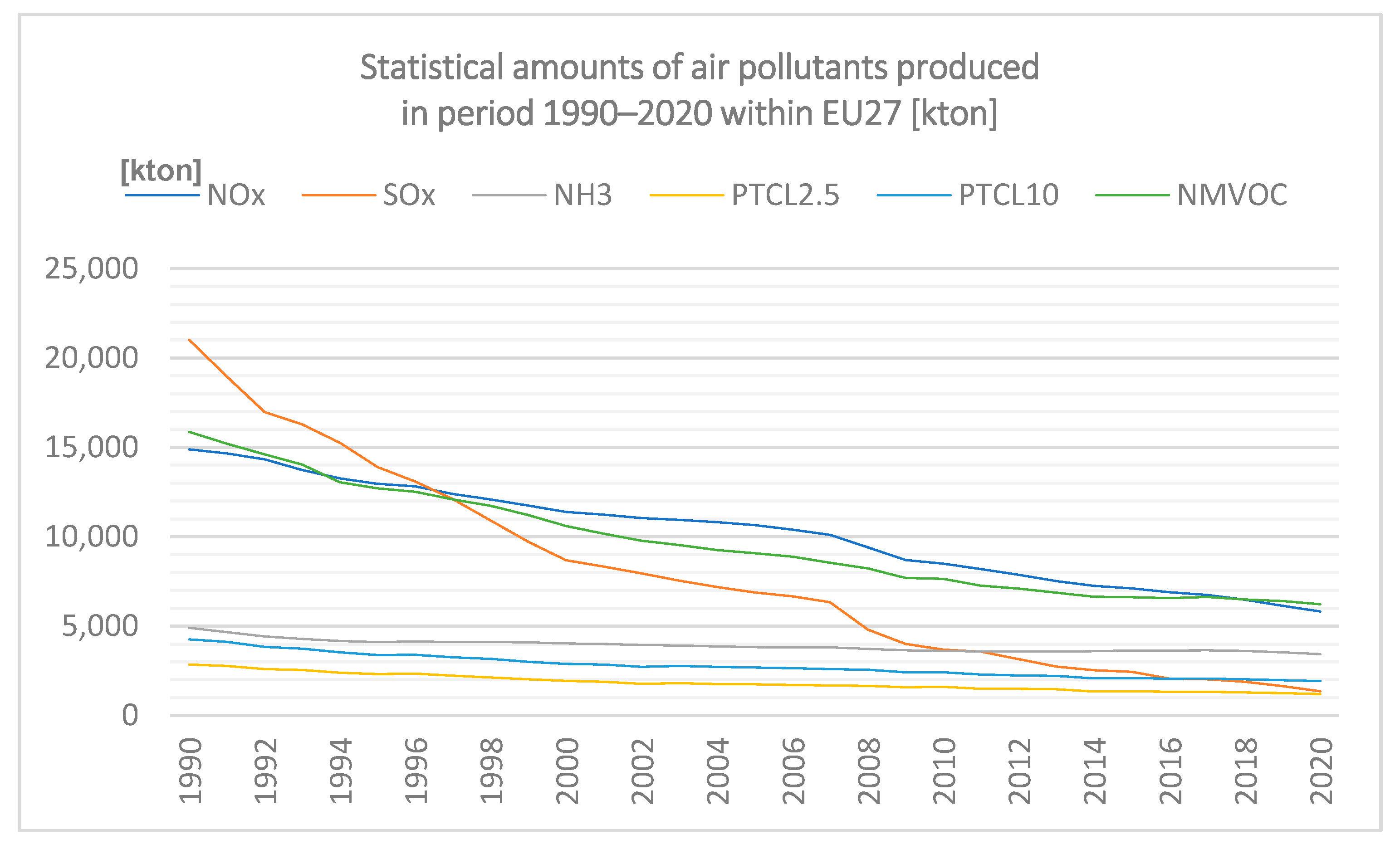
All input data used for further processing origin from databases of a Directorate-General of the European Commission (Eurostat 2022). The data refer to the national total for the entire territory and were drawn up on the base of fuel sold. They include the time period of 1990–2020 (Table 1).

Table 1.
Amounts of air pollutants produced by the transport sector in EU27 in the period 1990–2020 in tonnes (Eurostat 2022).
The data are graphically represented in Figure 1.
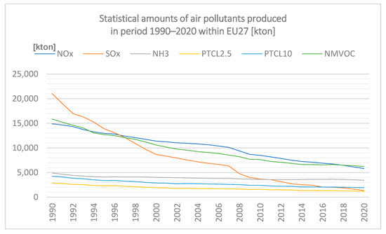
Figure 1.
Statistical amounts of air pollutants produced in the period 1990–2020 within EU27 in tonnes (processed according to Eurostat 2022).
3. Results
This section includes two predicting sets processed by help of a spreadsheet and neural network that processed the same input data described in Section 2.3. Each of the sets contains a table consisting of predicted results completed by a diagram showing development curves.
3.1. Spreadsheet-Predicted Amounts of Air Pollutants Produced in Period 2021–2050 within EU27
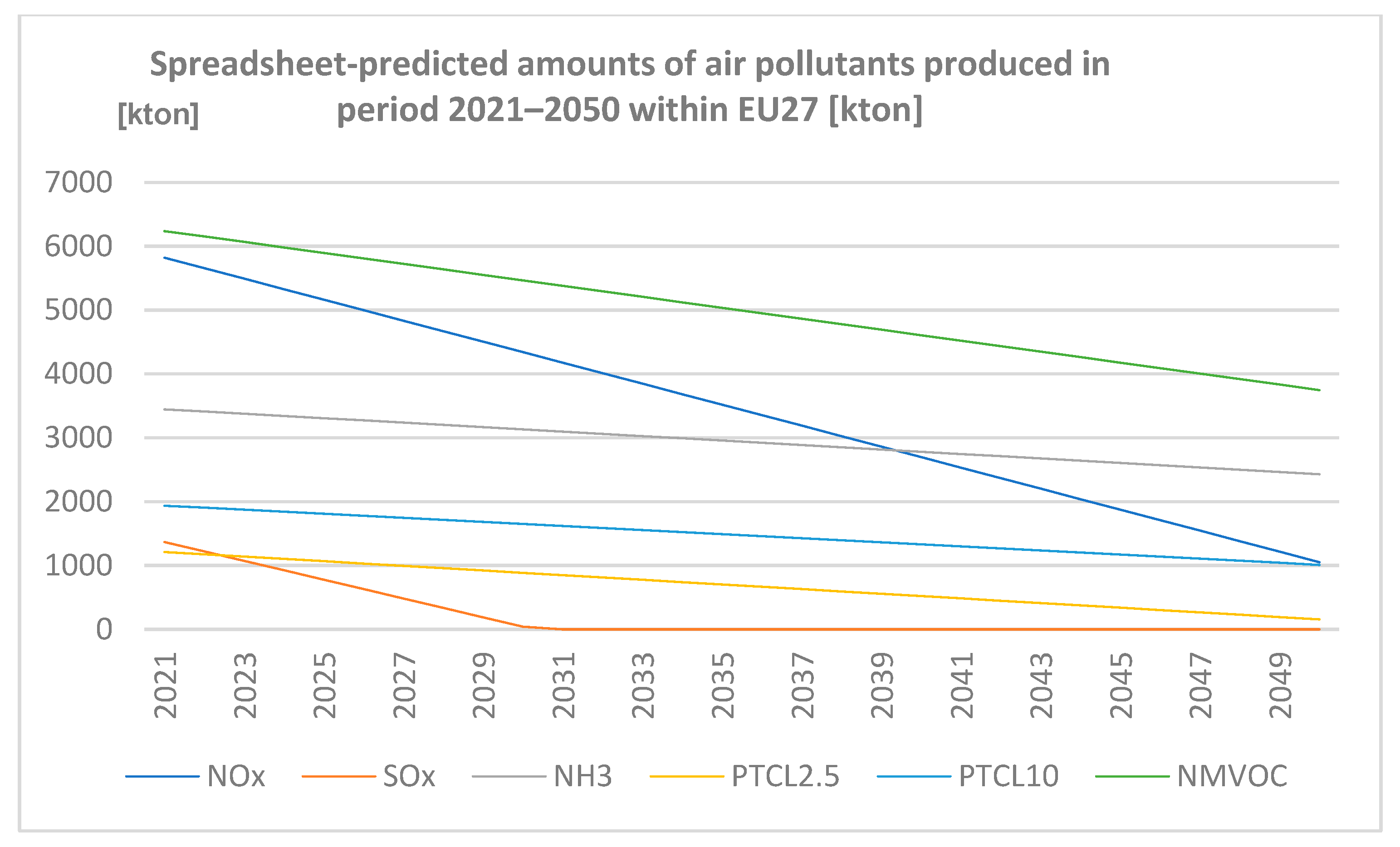
The first part of predicting a set of produced amounts of air pollutants was processed by means of the MS Excel spreadsheet. The statistical amounts of air pollutants produced in the period 1990–2020 within EU27 based on the Eurostat database from 2022 were used as input data (Table 2).
Table 2.
Spreadsheet-predicted amounts of air pollutants produced in the period 2021–2050 within EU27 (author’s own work).
The data are graphically represented in Figure 2.
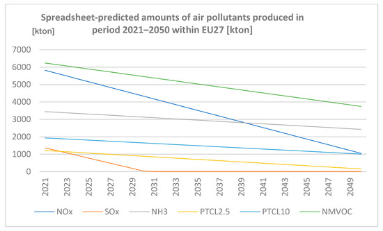
Figure 2.
Spreadsheet-predicted amounts of air pollutants produced in the period 2021–2050 within EU27 (author’s own work).
3.2. Neural Network-Predicted Amounts of Air Pollutants Produced in Period 2021–2050 within EU27
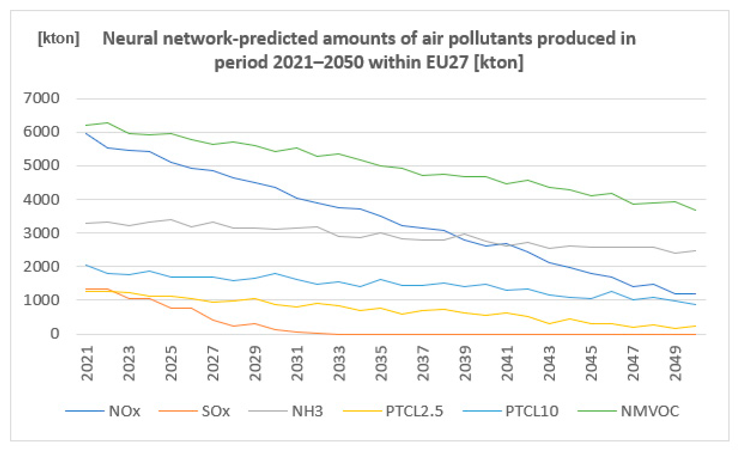
The second part of predicting the set of produced amounts of air pollutants is processed by means of the Orange software (v. 3.3, University of Ljubljana 2016, Slovenia) providing neural network algorithms. The statistical amounts of air pollutants produced in the period 1990–2020 within EU27 based on the Eurostat database from 2022 were used as input data as in the case of the spreadsheet base prediction (Table 3). The data are graphically represented in Figure 3.
Table 3.
Neural network-predicted amounts of air pollutants produced in the period 2021–2050 within EU27 (author´s own work).
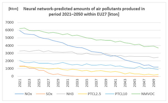
Figure 3.
Neural network-predicted amounts of air pollutants produced in the period 2021–2050 within EU27 (author´s own work).
The data are graphically represented in Figure 3.
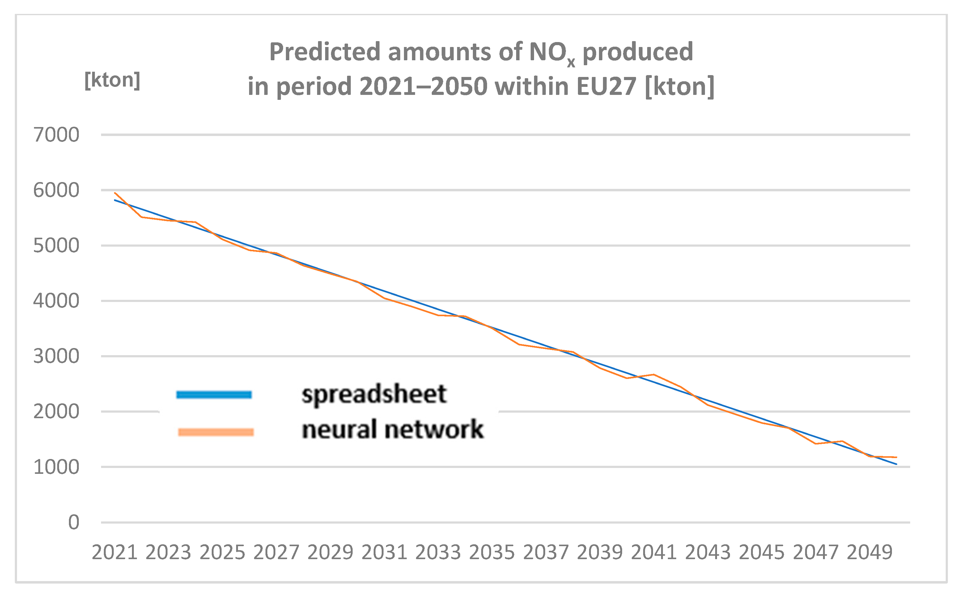
To obtain better comprehensibility of the above-figured results, couples of data series representing the same pollutants obtained with the help of two different predicting methods are discussed separately in the following section.
3.2.1. Amounts of NOx Produced in Period 2021–2050 within EU27 [Kton] Predicted by Spreadsheet and Neural Network
Amounts of NOx produced in the period 2021–2050 within EU27 (expressed in Kton) are represented in Figure 4.
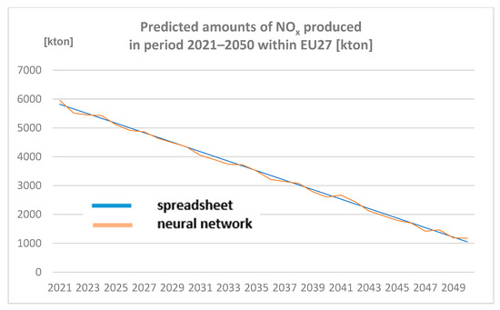
Figure 4.
Predicted amounts of nitrogen oxides (NOx) produced in the period 2021–2050 within EU27 [kton] (author´s own work).
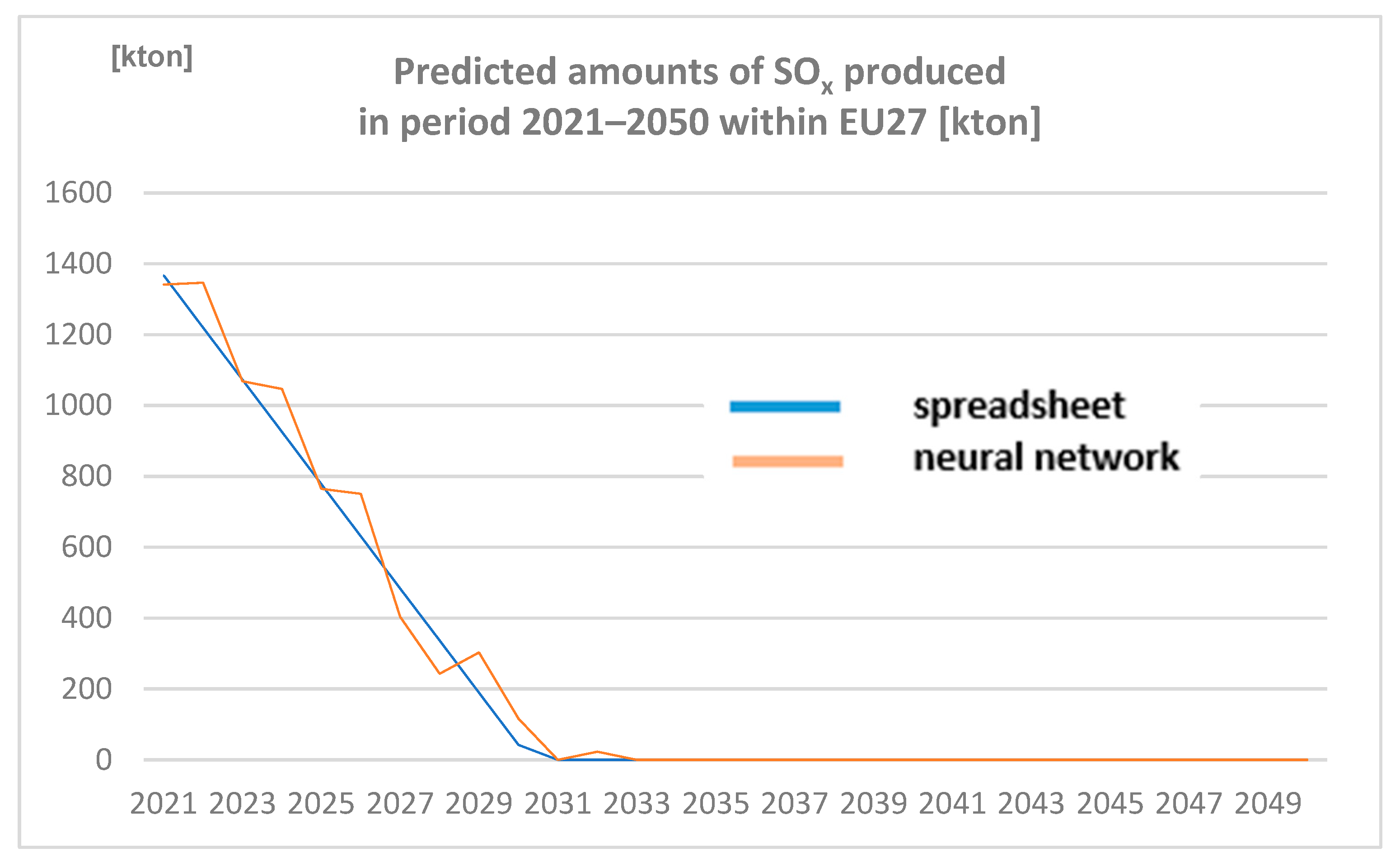
3.2.2. Amounts of SOx Produced in the Period 2021–2050 within EU27 [Kton] Predicted by Spreadsheet and Neural Network
Amounts of SOx produced in the period 2021–2050 within EU27 (expressed in Kton) are represented in Figure 5.

Figure 5.
Predicted amounts of sulphur oxides (SOx) produced in period 2021–2050 within EU27 [kton] (author´s own work).
Note: Values decreasing below zero (in 2031 spreadsheet; in 2033 neural network) are converted to 0 to not contain any negative values.
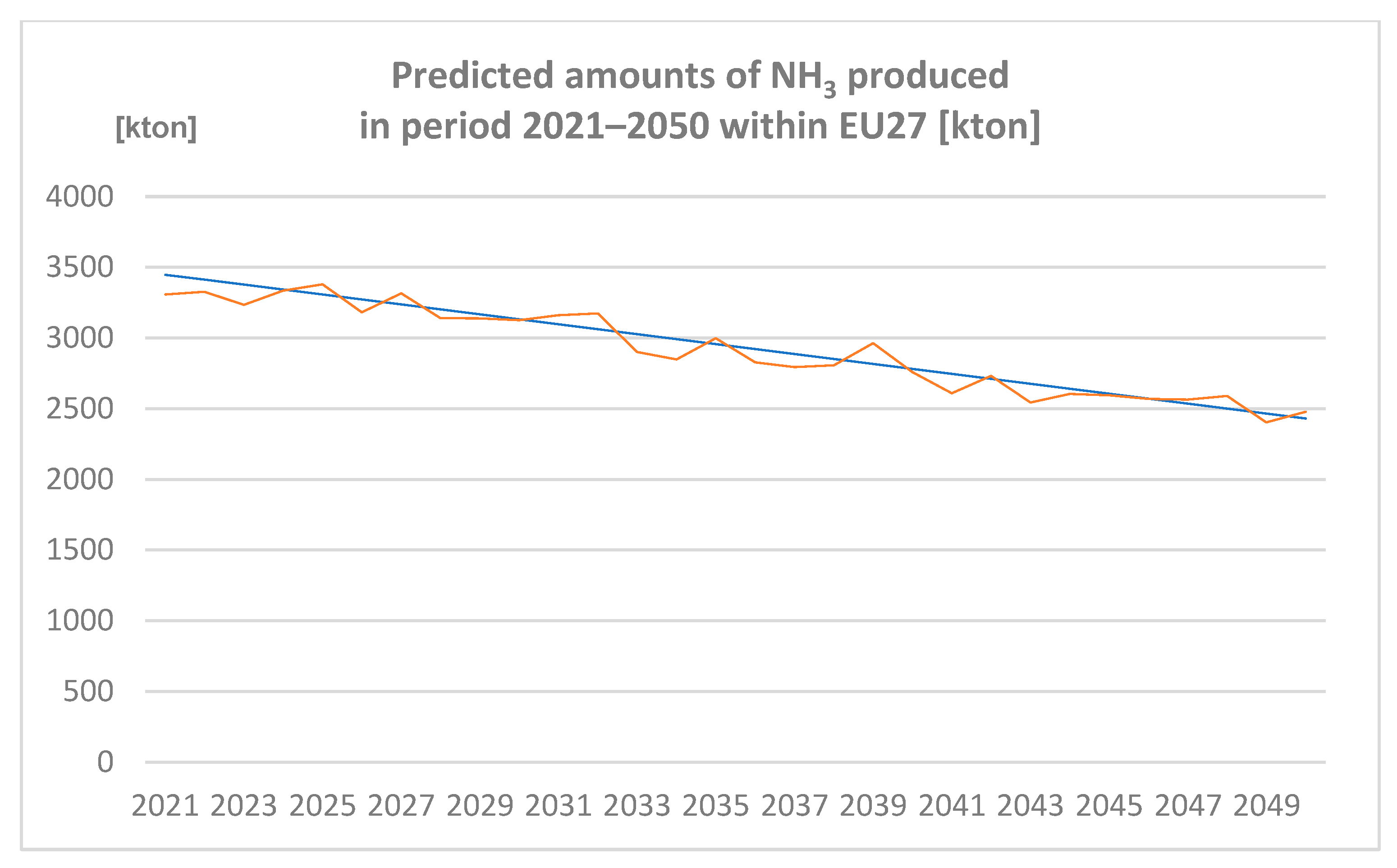
3.2.3. Amounts of NH3 Produced in the Period 2021–2050 within EU27 [Kton] Predicted by Spreadsheet and Neural Network
Amounts of NH3 produced in the period 2021–2050 within EU27 (expressed in Kton) are represented in Figure 6.
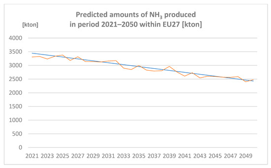
Figure 6.
Predicted amounts of ammonia (NH3) produced in the period 2021–2050 within EU27 [kton] (author´s own work).
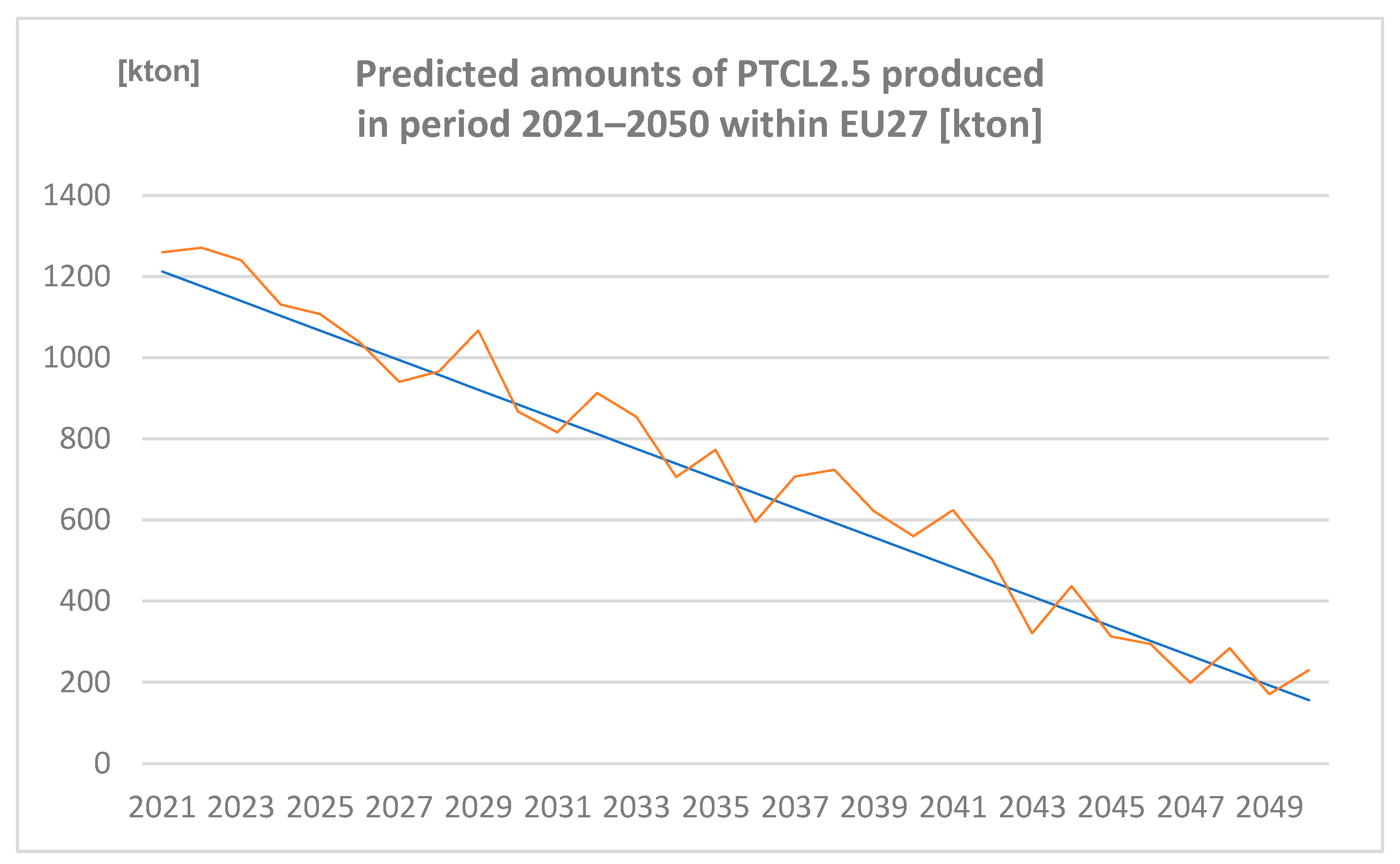
3.2.4. Amounts of PTCL2.5 Produced in the Period 2021–2050 within EU27 [Kton] Predicted by Spreadsheet and Neural Network
Amounts of PTCL2.5 produced in the period 2021–2050 within EU27 (expressed in Kton) are represented in Figure 7.
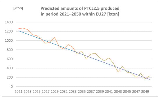
Figure 7.
Predicted amounts of particulates less than 2.5 µm (PTCL2.5) produced in the period 2021–2050 within EU27 [kton] (author´s own work).
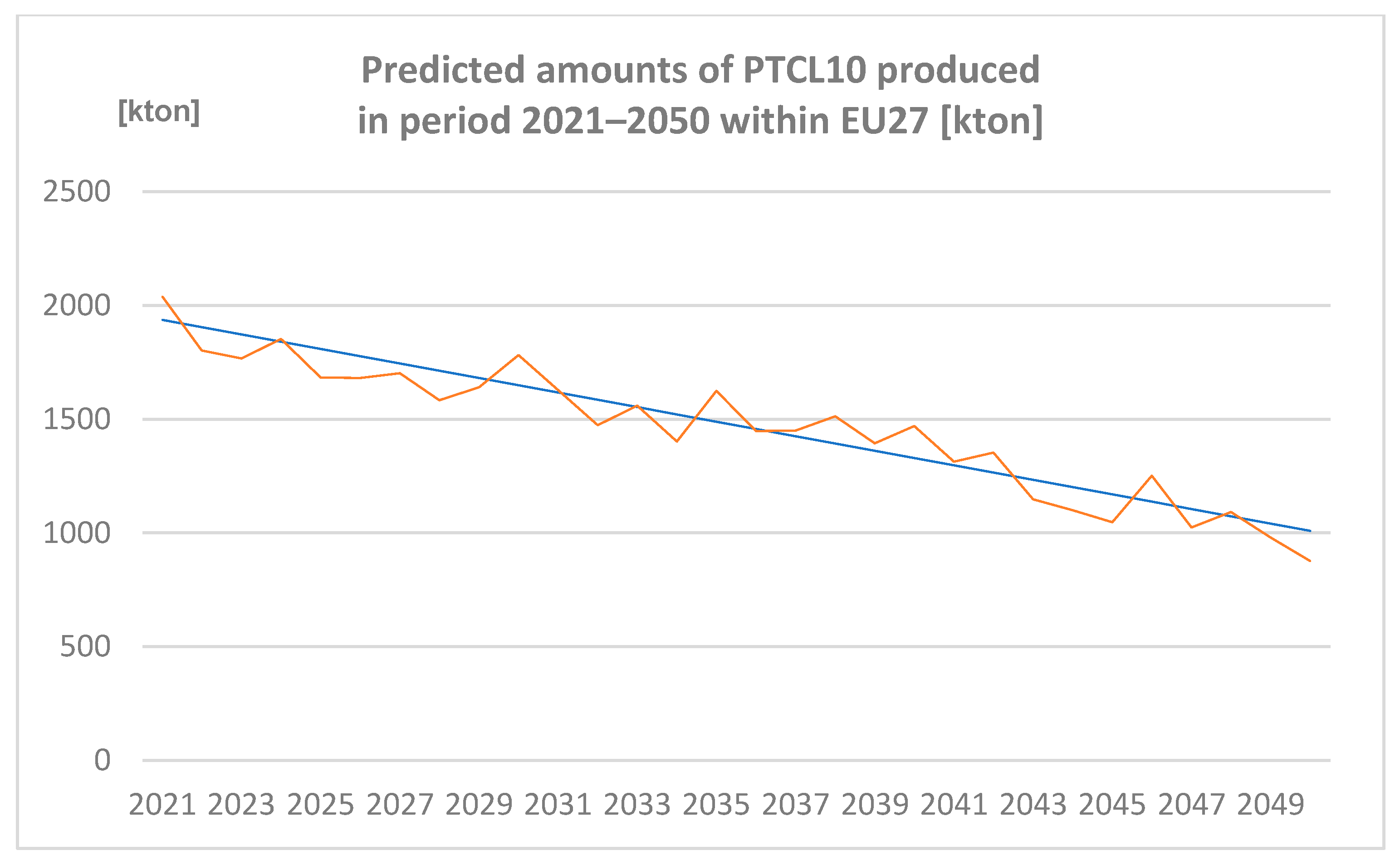
3.2.5. Amounts of PTCL10 Produced in the Period 2021–2050 within EU27 [Kton] Predicted by Spreadsheet and Neural Network
Amounts of PTCL10 produced in the period 2021–2050 within EU27 (expressed in Kton) are represented in Figure 8.
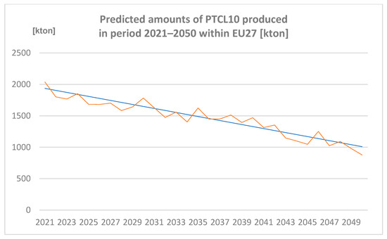
Figure 8.
Predicted amounts of particulates less than 10 µm (PTCL10) produced in the period 2021–2050 within EU27 [kton] (author´s own work).
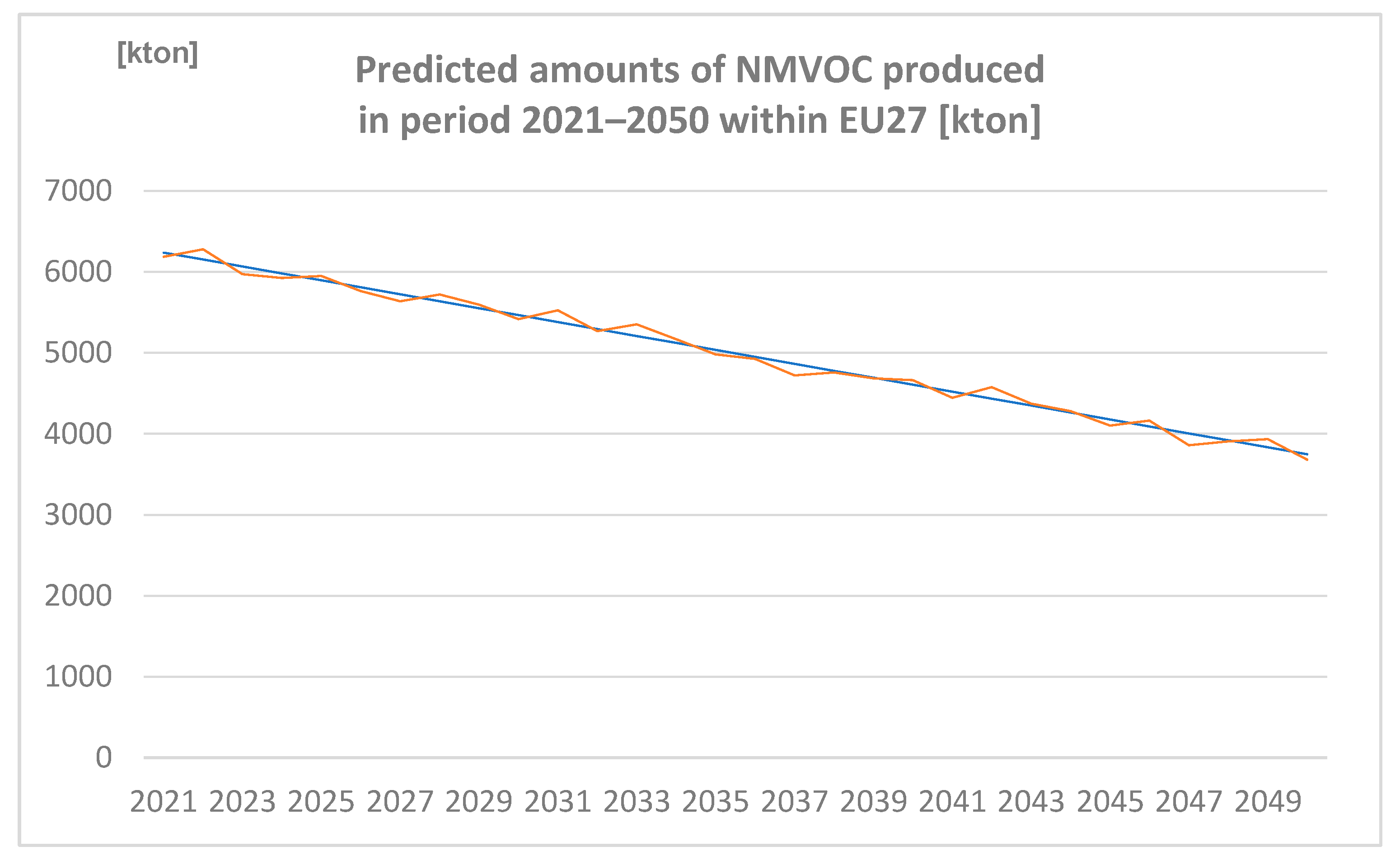
3.2.6. Amounts of NMVOC Produced in the Period 2021–2050 within EU27 [kton] Predicted by Spreadsheet and Neural Network
Amounts of NMVOC produced in the period 2021–2050 within EU27 (expressed in Kton) are represented in Figure 9.
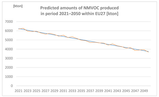
Figure 9.
Predicted amounts of non-methane volatile organic compounds (NMVOC) produced in the period 2021–2050 within EU27 [kton] (author´s own work).
Additionally, predicting by means of MS Excel´s Create Forecast Worksheet procedure provides an extension of the result sets by upper and lower trend (parameters Lower Endpoint and Upper Endpoint). Nevertheless, this additional information is not particularly within the scope of comparative analysis that represents the focus of this paper.
4. Discussion
The resulting diagrams (Figure 1, Figure 2 and Figure 3) cover three different data categories coming from the preceding tables: historical data (Figure 1) based on Eurostat data, predicted data (prognoses) calculated with the help of Excel´s Create Forecast Worksheet procedure (Figure 2), and data forecasted with the help of Orange software with neural networks (Figure 3). While the data taken over from the Eurostat databases provided the spreadsheet with inputs for processing the first type of prognoses (development trends), the columns of values calculated within the Orange neural network software were given into the spreadsheets additionally so that they could be formed into the integrated diagrams including dual curves.
The goal of this work was to find dissimilarities of results provided by spreadsheet exponential regression and neural network regression and, further, evaluation of usability both of them by means of comparative analysis and graphs. As a base, official data from Eurostat databases (GHG emissions and dependence on fossil fuels within the time period 1990–2020) [13] was used. The previous research [14] showed that neural networks represent the most convenient possibilities for prognosis and, generally, for prediction.
The relation between input and output data was probably too non-linear and complex to be described with the help of linear regression. However, classification results show that the use of logistic regression and neural network classification provide more or less similar results. In the case of regression, all error distributions were the lowest for function set {Standard, Featuretools} excepting MAPE (Mean Absolute Percentage Error). MAPE is not able to carry out calculations for data points of 0 value and, that is why MAPE represents a NaN (Not a Number) value in error calculating of the classification model. Aside from that, MAPE can cause information noise and, therefore, prognoses lower than a target value seem to be better because they provide smaller errors in comparison with the prognoses higher by the same value. It can also explain fluctuating among the feature (function) sets.
The obtained results show a moderate variance in the accuracy of predictions despite using two different methods. Another reason for analyzing exponential regression and neural network regression was to find whether the relation between input and output values was linear or non-linear. If the prognoses provided by neural networks are more accurate, the number of samples is probably enough to build a reliable computation model. When the neural network regression consistently performs better than linear regression, the relationship between input and output values would be non-linear at least to some level [15].
5. Conclusions
Predicting trends of pollutant production is not expected to give absolutely accurate answers because models designed on the perceptron neural networks basis substitute paradigmatic states of interpolating functions strongly dependent on the configuration of the network [16]. Processing the same input data sets and following outputting of highly similar values convincingly show that neural networks are usable for predicting pollutant production trends development in the same way as standard statistic predicting methods.
The general problem of evaluating tools in prediction is quite complicated. It is due to the fact that a complete theory and heuristics for statistical procedures are available for modeling over the given data [17]. In the case of neural networks, however, there are no heuristics that would clearly guide a procedure to the correct parameter settings for every kind of network. The theoretical setting of network parameters lies in their infinite combination. Within the scope of testing individual parameters, it is not possible to say that any combination of parameters has achieved the best results that the network could technically achieve [18]. The computational time of each set takes a long time, depending on the length of the time series and the complexity of the network architecture. This time can be on the order of hours on classical workstations. However, this solution implies the need for a large computational power or time capital for the computation [19]. Another problem consists of the selection of the architectures for analysis over the given time series. It cannot be generally said that only one architecture is suitable for analysis over transport-related time series. Rather, it can be observed that each architecture is suited to a different type of data in terms of the number of observations, its volatility, etc. [20]. On the other hand, any architecture is relatively easy to change and experiment with.
Neural networks are the alternative way to exact statistical methods within the field of predicting trends within transport planning as well as within other branches.
Funding
This research received no external funding.
Institutional Review Board Statement
Not applicable.
Informed Consent Statement
Not applicable.
Data Availability Statement
Data available in a publicly accessible repository. The data presented in this study are openly available, sources are stated in References.
Conflicts of Interest
The author declares no conflict of interest.
References
- Cristea, A.; Hummels, D.; Puzzello, L.; Avetisyan, M. Trade and the greenhouse gas emissions from international freight transport. J. Environ. Econ. Manag. 2013, 65, 153–173. [Google Scholar] [CrossRef]
- Llano, C.; Pérez-Balsalobre, S.; Pérez-García, J. Greenhouse Gas Emissions from Intra-National Freight Transport: Measurement and Scenarios for Greater Sustainability in Spain. Sustainability 2018, 10, 2467. [Google Scholar] [CrossRef]
- Antikainen, R.; Mattila, T. GHG Emissions and Fossil Fuel Dependency Scenario. In FreightVision—Scenario Building; 7th Framework Programme for Research; AustriaTech: Vienna, Austria, 2009. [Google Scholar]
- Tavasszy, L.; Piecyk, M. Sustainable Freight Transport. Sustainability 2018, 10, 3624. [Google Scholar] [CrossRef]
- Rich, J.; Brocker, J.; Hansen, C.O.; Korchenewych, A.; Nielsen, O.A.; Vuk, G. Report on Scenario, Traffic Forecast and Analysis of Traffic on the TEN-T, Taking into Consideration the External Dimension of the Union-Trans-Tools Version 2, Model and Data Improvements; DG TREN: Copenhagen, Denmark, 2009. [Google Scholar]
- Helmreich, S.; Mattila, T.; Antikainen, R.; Hansen, C.O.; Malinovský, V. Development of Strategic Scenarios of European Transportation. In Interim Report WP6.1 of FreightVision Project; AustriaTech: Vienna, Austria, 2011. [Google Scholar]
- EUROSTAT. Agriculture, Forestry and Fishery Statistics. 2016. Available online: https://ec.europa.eu/eurostat (accessed on 4 September 2022).
- Sajid, M.J.; Khan, S.A.R.; Gonzalez, E.D.R.S. Identifying contributing factors to China’s declining share of renewable energy consumption: No silver bullet to decarbonisation. Environ. Sci. Pollut. Res. 2022, 1–16. [Google Scholar] [CrossRef] [PubMed]
- Neubauer, J. Periodicita v Časové Řadě, Její Popis a Identifikace, Exponenciální Vyrovnávání (Periodicity in Time Series, its Description, and Identification, Exponential Smoothing), Study Materials; University of Defence: Brno, Czech Republic, 2020; pp. 14–16. Available online: https://k101.unob.cz/~neubauer/pdf/ekon_casove_rady_periodicita.pdf (accessed on 17 August 2021). (In Czech)
- Kačer, P. Vícevrstvá neuronová síť (Multi-Layer Neural Network). Bachelor´s Thesis, Department of Control and Instrumentation, Faculty of Electrical Engineering and Communications, Brno University of Technology, Brno, Czech Republic, 2013. (In Czech). [Google Scholar]
- Melart, S. Microsoft Office 2016: The Complete Guide; CreateSpace Publishing: Scotts Valley, CA, USA, 2015; ISBN 9781519282347. [Google Scholar]
- Dobešová, Z. ORANGE—Praktický Návod Do Cvičení Předmětu; Palacký University Olomouc: Olomouc, Czech Republic, 2022. (In Czech) [Google Scholar]
- Brandejský, T. Floating Data Window Movement Influence to Genetic Programming Algorithm Efficiency. In Computational Statistics and Mathematical Modeling Methods in Intelligent Systems, Proceedings of the 3rd Computational Methods in Systems and Software; Silhavy, P., Ed.; Springer: Cham, Switzerland, 2019; Volume 2, pp. 24–30. ISBN 978-3-030-31361-6. ISSN 2194-5357. [Google Scholar]
- Sajid, M.J. Machine Learned Artificial Neural Networks vs. Linear Regression: A Case of Chinese Carbon Emissions. In IOP Conference Series: Earth and Environmental Science, Proceedings of the 4th International Conference on Environmental and Energy Engineering, Sanya, China, 12–15 March 2020; IOP Publishing Ltd.: Bristol, UK, 2020; Volume 495. [Google Scholar] [CrossRef]
- Hallman, J. A Comparative Study on Linear Regression and Neural Networks for Estimating Order Quantities of Powder Blends. Master’s Thesis, School of Electrical Engineering and Computer Science, KTH Royal Institute of Technology, Stockholm, Sweden, 2019; pp. 49–53. Available online: http://www.diva-portal.org/smash/get/diva2:1383464/FULLTEXT01.pdf (accessed on 15 June 2022).
- Hlaváč, V. Neural Network for the identification of a functional dependence using data preselection. Neural Netw. World 2021, 31, 109–124. [Google Scholar] [CrossRef]
- Nakhaei, F.; Mosavi, M.R.; Sam, A.; Vaghei, Y. Recovery and grade accurate prediction of pilot plant flotation column concentrate: Neural network and statistical techniques. Int. J. Miner. Process. 2012, 110–111, 140–154. [Google Scholar] [CrossRef]
- Malinovský, V. Predicting Trends in Cereal Production in the Czech Republic by Means of Neural Networks. AGRIS On-Line Pap. Econ. Inform. 2021, 1, 87–103. [Google Scholar] [CrossRef]
- Svítek, M. Quantum multidimensional models of complex systems. Neural Netw. World 2019, 29, 363–371. [Google Scholar] [CrossRef]
- Malinovský, V. Comparative analysis of freight transport prognoses results provided by transport system model and neural network. Neural Netw. World 2021, 31, 239–259. [Google Scholar] [CrossRef]
Publisher’s Note: MDPI stays neutral with regard to jurisdictional claims in published maps and institutional affiliations. |
© 2022 by the author. Licensee MDPI, Basel, Switzerland. This article is an open access article distributed under the terms and conditions of the Creative Commons Attribution (CC BY) license (https://creativecommons.org/licenses/by/4.0/).