Abstract
The tourist industry is consistent with the new development paradigm and plays a crucial role in regional economic growth. At the same time, several areas of China have developed tourism as a vital industrial pillar. Analysing and examining the elements that affect the tourist industry in this setting has significant theoretical and practical implications. The dependent variable for this study is the tourist income for Guizhou Province from 2006 to 2019. A total of Eight variables are chosen as independent variables, including the distance travelled by rail and by road, the number of civil flights, the number of travel agencies, the overall number of tourists, the disposable incomes of both urban and rural residents, the number of tertiary industry workers, and the volume of foreign direct investment. The eight independent variables are discovered to favourably impact tourist revenue through the use of factor and regression analysis. Based on the study’s findings, this article suggests that (1) crisis management should be strengthened, and tourist businesses should be advised to become more active rather than passive, (2) infrastructure development should be enhanced for supporting tourism and directing the growth of the rural tourist industry in the area, and (3) the use of digital technologies should be enhanced and the speed of building intelligent tourism should be increased.
1. Introduction
The growth of the tourist sector is crucial for opening up new avenues for the repatriation of foreign currencies and accelerating cash flow. On the other hand, the increased liquidity of currency turnover leads to a rise in national revenue and capital accumulation, laying the groundwork for international tourism’s growth and offering the necessary management experience [1]. An important measure of how far a place has developed its tourist industry is the number of foreign currency revenues. This is because regional tourism consumption, which accounts for a significant portion of the growth in tourism revenues from foreign consumption, can be directly distinguished from foreign exchange earnings, and can therefore be used to objectively explain why a region is attractive to foreign consumption [2]. Of course, infrastructure, the mainstay, is also crucial to the rise in tourism-related earnings. The most important part of regional tourism growth is the infrastructure level, which directly affects how many visitors the area may expect to receive in the future [3].
Transportation, building, communications, commerce, catering, culture, and entertainment are just a few of the sectors covered by the tourism business. Tourism may also be a labour-intensive sector of the economy, requiring a lower threshold of workers and a more varied range and quality of employment, which can absorb a significant amount of labour and alleviate some social pressure [4]. As a result, tourism plays a significant role in the macroeconomy [5]. Tourism growth may also ease the regional movement of information, logistics, and money. Growing the tourism industry allows for the promotion of additional employment and the preservation of social order. Previously, a Canadian professor ran a methodical simulation and extrapolated that for every extra US$30,000 that the tourist sector brought in, one new direct job would be created, and the number of indirect employment would rise to around five [6]. There are more excellent prospects for tourist growth thanks to China’s overall industrial structure, which has been consolidated, improved, and developed through time [7]. In order to promote the integration of the primary, secondary, and tertiary sectors and to contribute to the proper growth of the national economy, an optimised industrial structure demands a majority proportion of the tertiary sector in the national economy [8]. Due to the pivotal role that tourism can play in the process of optimising the industrial structure, such as in the macro framework of promoting orderly economic flows which can generate more lucrative foreign exchange surpluses and give the nation’s sustainable development a boost [9], the development of tourism is also inextricably linked to the optimisation of the industrial structure.
As can be seen from the discussion above, the features of the tourist sector have a significant correlation with the industry’s size and complexity. There are six critical components of tourist development: food, lodging, transportation, travel, shopping, and entertainment. The “six elements of tourism” are the tourist industry’s fundamental components and material circumstances, in addition to more forgiving factors such as services, workers, and innovation [10]. Therefore, concentrating on these characteristics alone is insufficient if a place aims to achieve sustained and dependable tourist growth [11]. What elements, therefore, affect the growth of the tourist industry, and do various aspects affect the tourism economy? These issues may be appropriately analysed and investigated to identify the significant drivers of the tourist economy, which is crucial for developing the sector’s transformational potential and transformation and upgradation. Researchers have already begun to look at and analyse these difficulties. In earlier research, academics have tended to emphasise the significance of transportation infrastructure in fostering the growth of the tourist industry, seeing transportation infrastructure as a crucial component determining tourism [12]. Road mileage and civil aviation aircraft traffic are two elements that have a direct influence on tourism [13,14].
Additionally, it is well known that one of the critical determinants of the economic growth of tourism is the level of consumption of the local populace in the province where the tourist destination is located [15]. The amount of consumption in a location may be determined by looking at the disposable income of both urban and rural populations [16]. From the body of current research, experts have concentrated more on how physical factors, such as tourist infrastructure and resources, affect the growth of the tourism industry [17]. Since much of the literature focuses on a single location or city, the findings may not be broad, and there is a dearth of studies on the influence of soft variables such as innovation and practitioners on the growth of the tourist sector. This essay will use Guizhou Province’s entire tourist industry growth as its study topic. Furthermore, we will research which variables significantly contribute to the growth of the tourist industry in Guizhou Province using factor analysis and regression analysis.
In recent years, Guizhou province’s entire tourist model and consumer experience have evolved toward personalization, diversity, and quality, which has fuelled Guizhou’s overall economic growth and promoted structural optimization. The ratio of Guizhou’s tourist industry’s GDP contribution from 2010 to 2019 (Figure 1) shows that the industry’s GDP contribution rose from 23.48% in 2010 to 73.46% in 2019. Due to the rising tourism production in Guizhou province after the associated upgrading and optimization of the tourist structure, these numbers demonstrate a solid predictability in the industry’s growth.
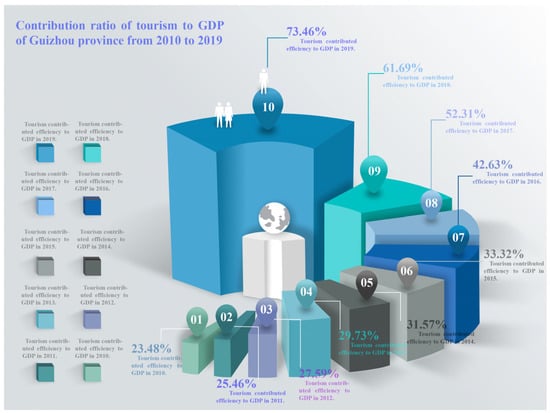
Figure 1.
Contribution ratio of tourism to GDP of Guizhou province from 2010 to 2019. (Data source: Guizhou Provincial People’s Government).
Meanwhile, the following essay examines the path of Guizhou’s tourist development in terms of the benefits of Guizhou’s tourism resources and the high-quality growth of Guizhou’s tourism. As long as Guizhou province fully commits to understanding the two fundamental red lines of resources and consumption, it is anticipated that Guizhou province will continue to move in the direction of high-quality tourism development. This is based on the measurement of the experimental data in this paper. More international visitors may be attracted by the upgraded tourism model, which can also provide Guizhou province’s economy with a more steady boost.
2. Overview of Tourism Resources in Guizhou Province
An introduction to Guizhou’s tourist resources is given below in light of the discussion above. Currently, Guizhou province contains three autonomous prefectures and six prefecture-level cities (Figure 2). The tourism market is progressively being standardised and improved, the overall comprehensive strength is considerably growing, and the tourist customer experience is steadily improving with the continued growth of Guizhou’s economy [18]. There are currently 48 regional minority groups residing in Guizhou, and these areas make up enormous village sites that will provide the impetus for tourism development in Guizhou province, paving the way for Guizhou’s tourism to move towards high standards. The integrity of the relevant infrastructural support directly determines the future expectations of tourism consumption, and the current state of Guizhou’s tourism resources echoes this thesis [19]. The following analyses the present state and features of the Guizhou province’s tourist resources from two angles.
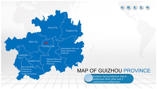
Figure 2.
Map of Guizhou Province. (The red dot is Guiyang, capital of Guizhou province).
2.1. Rich and Profound Intangible Cultural Heritage
Guizhou’s multi-ethnic population is more pronounced than its neighbouring provinces, accounting for a third of the population and 48 different ethnic minorities. This diversity of ethnic groups has given rise to various ethnic customs and some of the nation’s few remaining traditional ethnic village monuments [20].
Traditional types of multi-ethnic habitation are made easier in Guizhou’s hilly terrain, and the distribution pattern of “big mixed and tiny communities” has distinctive topographical features [21]. Due to the closeness to Guizhou and Yunnan and the interconnecting rivers and forests, the ethnic minorities were compelled to live in groups to adapt to their surroundings. In this setting, unique traditional villages have been maintained, even for millennia [22]. Geographical restrictions brought about by the terrain of the mountains and rivers have also boosted natural variety and aided in the emergence of ethnic and cultural diversity.
Guizhou has always played a significant role in the development of Chinese history, and due to its distinctive physical setting ancient strategists considered it a must-see. After centuries and millennia of integration, the Chinese and other ethnic groups (the Qiang, Miao and Yao, and Baiyue) have come to Guizhou from various historical periods and together developed a multi-ethnic “cultural symbiosis” in Guizhou, which also serves as an excellent genealogical resource for the growth of cultural industries in ethnic minority areas today [23].
A total of 713 intangible cultural heritage protection lists have now been created by Guizhou Province, ranging from the first to the fifth (Figure 3), with 118 designated national intangible heritage protection lists. The vast potential of Guizhou’s cultural resources, which will serve as a solid foundation for the next phase of the country’s cultural revitalization, is evident from the fact that the majority of the intangible cultural heritage listings are found in village locations populated by ethnic minorities.
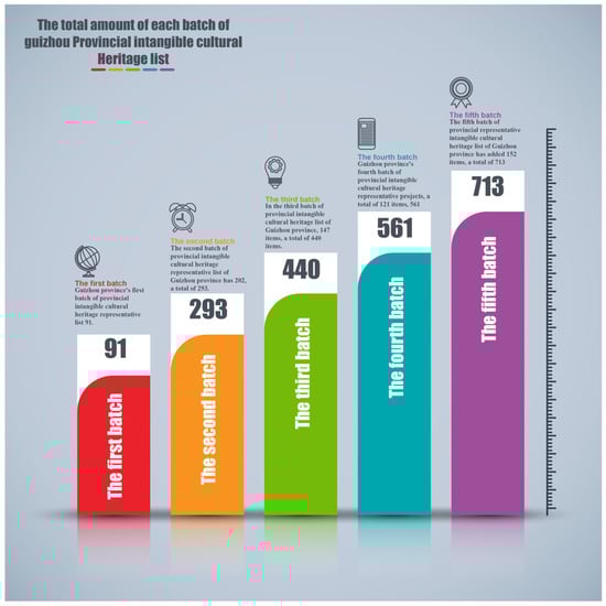
Figure 3.
Quantity of five batches of provincial intangible Cultural Heritage list in Guizhou Province. (Data source: Guizhou Provincial People’s Government).
2.2. Diversified Tourism Resources in Ethnic Minority Areas
In addition to the accumulation of culture, tourism development is also inextricably linked to supporting primary resources. In particular, Guizhou, a minority region, has produced numerous traditional ethnic villages due to the coexistence of various ethnic groups. Each village has distinct characteristics, and after thousands of years of accumulation these villages are now a rare source of cultural tourism resources [24]. According to Figure 4, Guizhou has one-third of the country’s ethnic minorities, three autonomous prefectures, eleven autonomous counties, one hundred and ninety-three ethnic townships, and seventeen hereditary ethnic minorities. In addition, in 2014, 2017, and 2019, 312 ethnic minority villages received approval from the State Ethnic Affairs Commission to be designated as “Chinese Ethnic Minority Villages with Characteristics”, one of the highest numbers in China. The abundance of ethnic minorities’ tourism resources amply illustrates Guizhou’s significant tourist attraction potential, vast tourism growth potential, and a high degree of development predictability.

Figure 4.
Overview of ethnic minority areas in Guizhou Province. (Data source: Guizhou Provincial People’s Government).
The quality of travellers’ travel requirements is rising along with the times. People’s quest for a genuine travel experience has outgrown the classic carousel-tour sightseeing [25]. In Guizhou, traditional villages with such a rich historical and cultural legacy are inherently appealing to tourists because they allow them to experience both the historical splendour of the villages and the ethnic practises that are part of them. People who go through these traditional villages will be thrilled and joyful, breaking the old basic tourism style and offering them a more immersive, in-the-moment sightseeing experience [26].
In subsequent years, it is anticipated that tourist numbers will increase gradually due to Guizhou’s abundant ethnic and cultural tourism resources and attractions. However, since 2020, the New Crown plague has significantly impacted China’s tourist business, and domestic tourism is still slowly recovering from its enormous blow. Even after improving from 2020, the overall number of visitors and revenue in China’s domestic tourism sector by the end of 2021 still lagged well below 2019. In order to investigate a route out of current tourist development, we may thus look into the historical era of 2006–2019, which also has some implications for solving the current tourism conundrum.
3. Empirical Analysis of the Factors Influencing Tourism in Guizhou Province
3.1. Selection of Variables
Based on the above study, an empirical study of the variables was conducted by combining data related to the total tourism revenue, road mileage, civil aviation flights, number of travel agencies, the total number of tourists, disposable income of urban residents, disposable income of rural residents, employees in the tertiary industry, and the scale of foreign direct investment in Guizhou Province (Table 1).

Table 1.
Summary of data related to total tourism revenue, road mileage, civil aviation flights, number of travel agencies, the total number of tourists, disposable income of urban residents, disposable income of rural residents, number of employees in the tertiary industry, and scale of foreign direct investment in Guizhou Province.
Gross tourism receipts (R): Gross tourist revenues include profits from both local and overseas travel. The growth of the tourist sector is directly reflected in the volume of tourism income. As a result, tourist income is a crucial indicator of the health of China’s tourism industry [27]. It serves as the dependent variable in this essay.
Road route mileage (T): A tourism destination’s appeal to travellers is directly influenced by its accessibility. Family automobiles are becoming more and more common as people’s living standards rise, and “self-driving” has taken over as the preferred form of transportation. Tourists find a place more appealing if its road transportation system is better established [28]. Remarkably, the province of Guizhou has continuously developed its road system, which has greatly aided the growth of the tourist industry. Therefore, this paper takes road mileage as one of the variables affecting the tourism economy.
Civil flight flow (M): Air travel will be a common means of transportation if the distance between the source and the destination is too vast. Travel by air may significantly save time spent on tourist activities and improve time efficiency [29]. As a result, the growth of the tourist industry is influenced by the number of passengers on commercial aircraft.
Total tourism arrivals (P): Inbound and domestic travel are also counted in the overall number of visitors. As more people travel, the tourism sector, which is highly dependent on human labour, adapts, which boosts local tourism spending and boosts the overall economic output [30].
The number of travel agencies (A): The number of travel agents in the area represents the existing state of the region’s tourist business, where visitors arrive directly via travel agents for associated services based on tourism and produce relevant tourism-related spending with the help of travel agents [31]. It also indicates the state of a region’s vital auxiliary services and the quality of its primary services.
Disposable income per urban resident (D): The real money that urban inhabitants have available to them for everyday living is referred to as their “disposable income”. The most significant and often-used metric to gauge urban inhabitants’ income levels and conditions of life is the disposable income per urban resident [32]. Additionally, Guizhou Province’s urban population are the industry’s largest customer segment, and their disposable income directly influences the growth of the tourist industry.
Net income per capita of rural residents (I): Net income per farmer is defined as net income “estimated based on the rural population and reflecting the average income level of rural people in a nation or area”. Net income is the sum of all annual revenue earned by rural dwellers from all sources, minus any associated costs paid to achieve that. Residents in rural areas earn more money as society develops, and their quality of life is progressively improving [33]. Rural populations have also developed into crucial customers in China’s tourist industry. As a result, one of the key factors influencing the growth of Guizhou Province’s tourist industry is the disposable income of rural populations.
Tertiary sector employees (E): The expansion of the tourist sector requires a large workforce and the building of the required infrastructure and other hardware expenditures. Numerous employees are needed to work in the tourist services sector since it is a service- and labour-intensive industry [34]. If we want to foster tourism’s high-quality growth, we will eventually need the academic assistance of high-quality individuals in the tertiary sector.
The scale of foreign direct investment (F): In today’s world, foreign direct investment (FDI) is a fundamental form of international capital exchange and an effective technique for using foreign money. In general, increasing the use of foreign investment denotes higher chances for economic development, and often denotes an improvement in a nation’s position concerning its balance of payments, which stimulates the domestic economy. The foreign capital influx will raise overall societal demand. If there is still room for growth, businesses will raise production to be in line with that potential. However, economic development will be harmed if inflows of foreign money decline. Foreign capital inflows can boost a nation’s foreign reserves and foreign currency supply, reduce the current account deficit, and enlarge the balance of payments surplus [35].
3.2. Stability Test of ADF Data Series
The following conclusions can be drawn from the below table (Table 2):
Table 2.
ADF test table.
(1) For R, the t-statistic for the ADF test of this time series data is 7.051, with a p-value of 1.000 and critical values of −5.500, −4.072, and −3.493 for 1%, 5%, and 10%, respectively. Due to the fact that p = 1.000 > 0.1, the original hypothesis cannot be rejected, and the series is not smooth. The series was subjected to first-order difference and then an ADF test. The result of the ADF test on the data after first-order difference shows that p = 0.982 > 0.1, and so the original hypothesis cannot be rejected, and the series is not smooth; therefore, the series was subjected to second-order difference and then the ADF test. The result of the ADF test after second-order differencing shows that p = 0.041 < 0.05; therefore, there is more than 95% certainty of rejecting the original hypothesis, and the series is smooth.
(2) For A, the t-statistic of the ADF test for the time series data is −0.621, with a p-value of 0.978 and critical values of −5.118, −3.918, and −3.411 for 1%, 5%, and 10%, respectively. Due to the fact that p = 0.978 > 0.1, the original hypothesis cannot be rejected, and the series is not stationary. The series was subjected to first-order difference and then an ADF test. The results of the ADF test on the data after first-order differencing show that p = 0.012 < 0.05; therefore, there is more than 95% certainty that the original hypothesis is rejected, and the series is smooth at this point.
(3) For P, the t-statistic for the ADF test of the time series data was 9.272, with a p-value of 1.000 and critical values of −5.500, −4.072, and −3.493 for 1%, 5%, and 10%, respectively. Due to the fact that p = 1.000 > 0.1, the original hypothesis cannot be rejected, and the series is not smooth. The series was subjected to first-order difference and then an ADF test. The results of the ADF test on the data after first-order differencing show that p = 0.124 > 0.1; therefore, the original hypothesis could not be rejected, and the series was not stationary, so the series was subjected to second-order differencing and then the ADF test. The result of the ADF test after second-order differencing shows that p = 0.021 < 0.05; therefore, there is more than 95% certainty of rejecting the original hypothesis, and the series is smooth now.
(4) For T, the t-statistic of the ADF test for the time series data is −1.646, with a p-value of 0.774 and critical values of −5.118, −3.918, and −3.411 for 1%, 5%, and 10%, respectively. Due to the fact that p = 0.774 > 0.1, the original hypothesis cannot be rejected, and the series is not stable. The series was subjected to first-order difference and then an ADF test. The results of the ADF test on the data after first order differencing show that p = 0.568 > 0.1; therefore, the original hypothesis could not be rejected, and the series was not stationary. The series was subjected to second-order differencing and then an ADF test. The result of the ADF test on the data after second-order differencing shows that p = 0.001 < 0.01; therefore, there is more than 99% certainty that the original hypothesis is rejected, and the series is smooth at this point.
(5) For M, the t-statistic for the ADF test of this time series data is −0.684, with a p-value of 0.974 and critical values of −5.118, −3.918, and −3.411 for 1%, 5%, and 10%, respectively.
With p = 0.974 > 0.1, the original hypothesis cannot be rejected, and the series is not smooth. The series was subjected to first-order difference and then an ADF test.
The ADF test result of the data after the first order difference shows p = 0.001 < 0.01; therefore, there is a higher than 99% certainty of rejecting the original hypothesis, and the series is smooth now.
(6) For D, the t-statistic of the ADF test for the time series data is 14.647, with a p-value of 1.000 and critical values of −5.500, −4.072, and −3.493 for 1%, 5%, and 10%, respectively. Due to the fact that p = 1.000 > 0.1, the original hypothesis cannot be rejected, and the series is not smooth. The series was subjected to first-order difference and then an ADF test. The results of the ADF test on the data after first-order differencing show that p = 0.055 < 0.1; therefore, there is more than 90% certainty that the original hypothesis is rejected, and the series is smooth at this point. The ADF test result for the second-order differential data shows that p = 0.000 < 0.01, with more than 99% certainty of rejecting the original hypothesis, and the series is stable at this point.
(7) For I, the t-statistic for the ADF test of the time series data is −1.348, with a p-value of 0.876 and critical values of −4.884, −3.822, and −3.359 for 1%, 5%, and 10%, respectively. Due to the fact that p = 0.876 > 0.1, the original hypothesis cannot be rejected, and the series is not smooth. The series was subjected to first-order difference and then an ADF test. The results of the ADF test on the data after first-order differencing show that p = 0.137 > 0.1; therefore, the original hypothesis could not be rejected, and the series was not stationary, so the series was subjected to second-order differencing and then the ADF test. The ADF test result of the data after second-order differencing shows p = 0.006 < 0.01. Therefore, there is more than 99% certainty of rejecting the original hypothesis, and the series is smooth now.
(8) For E, the t-statistic of the ADF test for the time series data is −0.364, with a p-value of 0.988 and critical values of −5.118, −3.918, and −3.411 for 1%, 5%, and 10%, respectively. Due to the fact that p = 0.988 > 0.1, the original hypothesis cannot be rejected, and the series is not smooth. The series was subjected to first-order difference and then an ADF test. The ADF test result of the data after the first-order difference shows p = 0.000 < 0.01; therefore, there is a higher than 99% certainty of rejecting the original hypothesis, and the series is smooth at this time.
(9) For F, the t-statistic for the ADF test for this time series data is −3.515, with a p-value of 0.038 and critical values of −5.118, −3.918, and −3.411 for 1%, 5%, and 10%, respectively.
With p = 0.038 < 0.05, there is a higher than 95% certainty that the original hypothesis is rejected, and the series is smooth at this point.
In summary, the data for all variables are serially stationary, and can proceed to the next step of the empirical data study.
3.3. Exploring: Tourism Revenue and Tourism Visitor Numbers
In summary, through the ADF test of the time series data for the variables of total tourism revenue (R), number of travel agencies (A), the total number of tourists (P), road route mileage (T), number of civil flights (M), per capita disposable income of urban residents (D), per capita net income of rural residents (I), employees in the tertiary industry (E) and scale of foreign direct investment (F), the data are all serially smooth, and further analysis can be conducted. The relationship between tourism income and the number of tourists is explored below.
(1) Literature support.
Firstly, in Lu Liu’s “The impact of tourism numbers on domestic tourism income in China”, the author focussed on the impact of domestic tourism numbers on domestic tourism income in China by developing a one-dimensional linear regression model [36]. The author also introduced the dynamic process of the development of the number of domestic tourists and domestic tourism income in China, followed by the determination of the quantitative relationship between these variables using the Eviews software system to determine the linear regression function from the data information; then, the author conducted statistical tests on the credibility of the model and determined the significance of the variables from the relevant variables [36]. Based on the conclusions drawn, countermeasures and suggestions for improving China’s domestic tourism revenue were proposed to achieve a smooth growth of domestic tourism revenue [36].
Based on this author’s well-documented view, the number of tourist visitors is included in the tourism revenue impact variable and empirically studied in this paper.
(2) A brief description of the relationship between the two.
Tourism is an activity that requires the movement of people and consumption across regions, and the essential thing in this process is the participation of people; in short, it is the number of tourists which plays a crucial role in this process [37]. It is evident that without the participation of people and tourists, a region could not generate the so-called tourism income. Without the involvement of tourists in tourism, the various functions would not be able to perform their work and utility, they would not be able to function accordingly, and they would not be able to generate direct economic benefits, i.e., tourism revenue, as most scholars have openly argued and thought [38]. If the one-sided relationship between tourism visitor numbers and tourism revenue is too much, the so-called pseudo-debate between the two will fall into an infinite cycle of ‘chicken producing eggs and eggs producing chickens’, which is not conducive to the depth of tourism research and is not in line with conventional thinking.
Therefore, this paper insists on including the number of tourists in the variables that affect tourism revenue for empirical analysis.
3.4. Model Construction and Testing
3.4.1. Initial Model Setting
Based on the above influencing-factors analysis, the following multiple linear regression model will be established in SPSS 20.0 based on the relevant data, and the constructed model Equation (1) is as follows.
This is example one of an equation:
where R denotes total tourism revenue, A denotes the number of travel agencies, P denotes the number of tourists, T denotes road route mileage, M denotes civil flight passenger traffic, and D denotes urban residents’ per capita disposable income. I denotes rural residents’ per capita net income, E denotes tertiary industry employees, F denotes the scale of foreign direct investment, and μt is a random disturbance term. The data in the model were all obtained from the statistical yearbook data of the Guizhou Provincial Bureau of Statistics from 2006 to 2019.
Ln R = β0 + β1LnT + β2LnM + β3LnA + β4LnP + β5LnD + β6LnI + β7LnE + β8LnF + μt
3.4.2. Standardized Processing of Data
Due to the large number of variables selected in this paper, the non-uniformity of units, and different magnitudes between variables, direct data analysis is not possible, so standardisation is required, using summation and normalisation to convert to dimensionless data. The formula for standardisation of the data is given in Equation (2).
This is example two of an equation:
The purpose of summation normalisation is to let the ‘summation value’ be the reference standard, and all the data are all divided by the summation value, so that the resulting data is equivalent to the summation percentage; as in Equation (2), i.e., the ‘summation value’ of all the data is used as the unit, and all the data are all standardized. The summation value is divided by the ‘summation value’. In this paper, the data of all variables are standardised according to Formula (4) to eliminate the effect of dimensionality, and the data of variables are standardised to conform to the law of normal distribution (Figure 5), so that factor analysis and regression analysis can be carried out later. The basic situation of the data of the variables after standardisation is shown in Table 3.
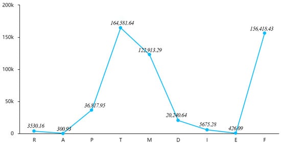
Figure 5.
Comparison chart of the mean values.
Table 3.
Base indicators.
The descriptive analysis describes the overall picture of the data employing medians. As can be seen from the above table (Table 3), there are no outliers in the current data; therefore, descriptive analysis can be carried out directly against the mean.
3.4.3. Data Testing
In this paper, eight independent variables affecting tourism economic development were selected, and factor analysis was required to facilitate the study and identify common patterns between the factors. Using factor analysis for information enrichment research, the research data were first analysed for suitability for factor analysis, as can be seen from the above table (Table 4): the KMO was 0.839, which is greater than 0.6, meeting the prerequisite requirements for factor analysis, implying that the data can be used for factor analysis research as well as meaning that the data passed Bartlett’s sphericity test (p < 0.05), indicating that the research data is suitable for factor analysis.
Table 4.
KMO and Bartlett’s test.
3.5. Factor Analysis
The below table analyses the factor extraction (Table 5) and the amount of information extracted from the factors. From the below table, we can see that a total of three factors were extracted from the factor analysis, and the variances explained by the rotation of these three factors were 40.953%, 32.122%, and 25.964%, respectively, and the cumulative variance explained by the rotation was 99.039%.
Table 5.
Variance Interpretation Rate Table.
The data in this study were rotated using the maximum variance rotation method (varimax) to find the correspondence between the factors and the study items. The above table shows how well the factors extracted information from the study items and the correspondence between the factors and the study items, from which it can be seen that all of the study items have a commonality value above 0.4, which means that there is a strong correlation between the study items and the factors and that the factors can extract information effectively. After ensuring that the factors could extract most of the information from the research items, the correspondence between the factors and the research items was then analysed (an absolute value of factor-loading coefficient greater than 0.4 means that there is a correspondence between the item and the factor).
Table 6 shows that the two-road mileage (T) and civil flights (M) converge on the first common factor, and according to the characteristics of these three variables, the first common factor can be named the infrastructure influence factor. The number of travel agencies (A) and the total number of tourists (P) converge on the second common factor, and according to the characteristics of these two variables, the second common factor can be named the influence factor of tourism flow. The four variables of urban disposable income per capita (D), rural net income per capita (I), tertiary industry employees (E), and foreign direct investment (F) converge on the third common factor, and according to the characteristics of these two variables, the third common factor can be named as the investment and consumption-influence factor. After extracting the three common factors, it is necessary to consider the linear relationship between each common factor and the variables, which can be obtained from the component score coefficient matrix, as shown in Table 7.
Table 6.
Factor load factor after rotation.
Table 7.
Component score coefficient matrix.
Once the three common factors have been extracted, it is necessary to consider the linear relationship between each common factor and the variables, which can be obtained from the matrix of component scoring coefficients, as shown in Table 7.
[Tips]
1: A research item corresponds to more than one factor. Due to this, time should be combined with professional knowledge to determine the specific attribution of that factor.
2: If a research item does not correspond to a factor, consider deleting the research item.
3: If a factor and a research item do not correspond, a reduction of one factor may be considered
4: If there is no correspondence between a research item and a factor, consider deleting the research item.
If factor analysis is used to condense information, then the ‘component score coefficient matrix’ table is ignored. If factor analysis is used to calculate weights, the relationship equation between the factors and the study items (based on standardised data to create a relationship expression) is created using the ‘component score coefficient matrix’ (Table 7), as shown in the formula below (3).
This is example three of an equation:
F1 = −0.346 × SN_M + 0.898 × SN_T + 0.876 × SN_A − 0.704 × SN_P + 0.200 × SN_D + 0.096 × SN_I + 0.076 × SN_E − 0.455 × SN_F
F2 = 0.661 × SN_M − 0.922 × SN_T − 0.353 × SN_A + 1.346 × SN_P + 0.036 × SN_D + 0.125 × SN_I + 0.198 × SN_E − 0.577 × SN_F
F3 = −0.044 × SN_M + 0.150 × SN_T − 0.478 × SN_A − 0.374 × SN_P − 0.032 × SN_D − 0.000 × SN_I − 0.057 × SN_E + 1.488 × SN_F
F2 = 0.661 × SN_M − 0.922 × SN_T − 0.353 × SN_A + 1.346 × SN_P + 0.036 × SN_D + 0.125 × SN_I + 0.198 × SN_E − 0.577 × SN_F
F3 = −0.044 × SN_M + 0.150 × SN_T − 0.478 × SN_A − 0.374 × SN_P − 0.032 × SN_D − 0.000 × SN_I − 0.057 × SN_E + 1.488 × SN_F
When the line suddenly becomes smooth, the number of factors from steep to smooth is the reference number of factors extracted. The rubble diagram only assists in the decision-making of the number of factors, and the actual study is more based on professional knowledge combined with the situation of the correspondence between the factors and the study items, and the comprehensive weighing judgment to arrive at the number of factors (Figure 6).
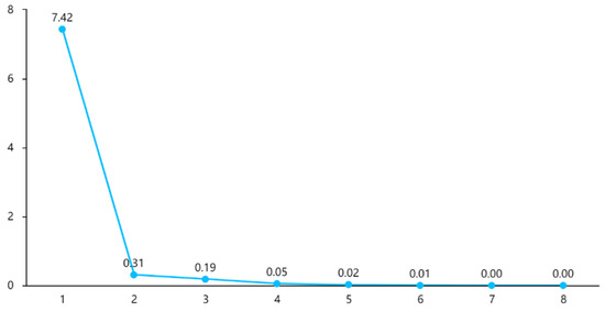
Figure 6.
Gravel diagram.
3.6. Linear Regression Analysis
From the above table (Table 8), F1, F2, and F3 were used as independent variables, while SN_R (total tourism revenue) was used as the dependent variable for the linear regression analysis from above table; from this, model Equation (4) can be derived.
Table 8.
Results of linear regression analysis (n = 14).
This is example four of an equation:
SN_R = 0.071 + 0.035 × F1 + 0.060 × F2 + 0.026 × F3
The model R-squared value of 0.985 implies that F1, F2, and F3 can explain 98.5% of the variation in SN_R (total tourism revenue). An F-test of the model revealed that the model passed the F-test (F = 221.321, p = 0.000 < 0.05), which means that at least one of F1, F2, and F3 would have a meaningful relationship on SN_tourism total tevenue (R), with a regression coefficient value of 0.035 for F1 (t = 11.989, p = 0.000 < 0.01), implying that F1 would have a significant favourable influence relationship on SN_R (total tourism revenue). The regression co-efficient value of F2 is 0.060 (t = 20.886, p = 0.000 < 0.01), implying that F2 will have a significant positive effect on SN_R (total tourism revenue). The regression coefficient value of F3 is 0.026 (t = 9.166, p = 0.000 < 0.01), implying that F3 will have a significant positive effect on SN_R (total tourism receipts) and has a significant favourable-influence relationship.
To summarise the analysis, it can be seen that F1, F2, and F3 significantly positively affect SN_R (total tourism revenue).
From the below graph (Figure 7) and table (Table 9), it can be seen that linear regression analysis was carried out with F1, F2, and F3 as the independent variables and SN_R as the dependent variable. The below table shows that the model R-squared value is 0.985, implying that F1, F2, and F3 can explain 98.5% of the variation in SN_R.
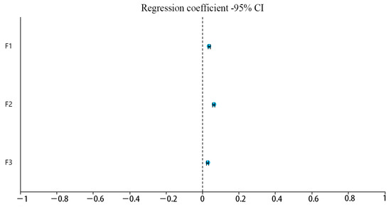
Figure 7.
Regression coefficient 95% CI.
Table 9.
Model summary (intermediate process).
From the above table, the model was found to pass the F-test (F = 221.321, p = 0.000 < 0.05) when the model was tested (Table 10), which means that the model construction is meaningful.
Table 10.
ANOVA table (intermediate process).
4. Analysis of the Factors Influencing Tourism Development in Guizhou Province
The linear regression analysis above shows that the three public factors, the infrastructure impact factor, the tourism flow impact factor and the investment and consumption impact factor, all have a significant positive relationship to total tourism receipts. However, the three public factors are extracted from eight independent variables which, on the other hand, also indicate that the number of travel agencies (A), the total number of tourists (P), road route mileage (T), civil flight movements (M), disposable income per urban resident (D), net income per rural resident (I), tertiary industry employees (E), and foreign direct investment (F) also have a more outstanding contribution to tourism income. Based on the results obtained from the above empirical study, the model results graph is supplemented by a new model relationship graph (Figure 8), which illustrates the relationship between the two.
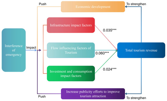
Figure 8.
Model relationship between infrastructure impact factor, tourism flow impact factor, and investment and consumption impact factor in Guizhou Province. (“***” indicates the regression coefficient).
(1) Impact analysis of total tourism revenue in Guizhou Province.
The overall development of total tourist revenues and the percentage of tourism’s contribution to the GDP are directly impacted by changes in the incremental or decremental effects of tourism variables [39]. In light of this, the consistency of total tourist income serves as a clear barometer of the local economy’s health and its associated social activities. However, the reasonably elastic status of tourism-related total revenue varies in a meaningful way in response to adjustments in the relevant variables [40]. That is, the congruence of the driving forces of infrastructure, traveller flows, investment, and consumption will directly affect the expansion of tourism-related earnings as a whole. The entire tourism infrastructure must be utilised as a starting point to boost tourism growth, concentrating on the quality of services, the need to make tourist sites more alluring, and the accuracy of consumer preferences [41]. The construction of auxiliary facilities for consumption and investment occurs concurrently with efforts to strengthen the pertinent critical support, directly affecting how much money is generated from tourism.
(2) Impact Analysis of Tourism Traffic in Guizhou Province
The number of visitors is a vital sign of how a region’s tourism industry is doing, since it directly affects the total tourism consumption pull and provides a reliable estimate of the region’s level of tourism appeal [42]. In general, it is vital to expand regional support services and the fundamental execution of the quality of services, as these factors will directly influence the number of visitors in the next year and the overall stability of the statistics of tourism frequency [43]. Today’s tourism relies on human activity, necessitating a variety of service amenities to satisfy customer demand for maximum usefulness. The link between the three variables in the model is also clear, with tourist flows having a more considerable influence than infrastructure impacts, investment impacts, and consumption impacts. This is because tourist flows exhibit specific economic characteristics, and their magnitude may be used to calculate the extent of the tourism economy’s output value [44].
5. Measures and Suggestions to Enhance Tourism Revenue in Guizhou Province
Based on the analysis of the factors influencing the tourism economy in Guizhou Province in this paper, we believe that we can start from the following aspects in order to promote the development of the tourism economy better.
(1) Strengthen crisis management and guide tourism enterprises to change from reactive to proactive.
We should boost field research to better understand business challenges and implement targeted initiatives. In response to the challenges caused by the pandemic, tourist-management departments might form research teams to carry out the study across many cities (counties). Guizhou’s tourism businesses will be better able to react swiftly to the epidemic’s effects and turn the crisis into an opportunity if they have a thorough understanding of the losses incurred by cultural and tourism businesses during the epidemic, as well as the challenges and issues encountered in resuming work and production [45]. Favourable tourist policies should also be introduced, and coupons for cultural and tourism consumption should be provided to assist businesses in regaining their faith in development.
To successfully assist businesses in overcoming challenges, we shall practice various preferential policies. More “Colored Guizhou Winter Tourism Consumption Vouchers” will be distributed. We will create special incentives and support policy measures via the Colorful Baby and One Code Guizhou platforms to encourage the growth of cultural and tourist firms and help them overcome their challenges. In order to aggressively execute a tourist source-driven strategy, several favourable tourism policies were implemented at the same time. Preferential tourist policies have been established, including reduced and halved scenic location entry prices [46]. Particular preferential policies have been implemented for important tourism visitor sources. Preferred policies for special trains, preferential policies for tickets to specific hot springs, and free admission rules for medical and disease control workers in particular hotspots may all be implemented to enhance the number of foreign visitors visiting Guizhou province.
The epidemic policy should be adequately publicised to stop the public from panicking about the outbreak. The tourist industry’s impact on the economy must be well understood, and we must swiftly educate the public with the most recent and pertinent information. To raise the level of service provided by the tourist industry and guarantee the steady growth of the cultural tourism sector, complaints about the industry should be treated with care. At the same time, we will keep enhancing our level of customer care to raise visitor happiness successfully.
(2) Strengthen tourism support facilities and guide the development of a regional rural tourism economy.
The following steps can be taken to achieve this goal: Coordinate the infrastructure development for rural tourism. Improve the road grade quality in picturesque tourist locations, while focussing on finding a solution to the road construction issue in important and rural tourist destinations [47]. Encourage the organic integration of urban and rural transportation and the integration of passenger transportation services. Resolve issues with water shortages, water cuts, and poor water quality in specific rural and touristic locations. Compile and enhance the results of drinking water safety in rural areas. The treatment of rural waste and sewage in tourist regions should be prioritised, with the thorough rehabilitation of the rural habitat environment and the building of attractive communities. Increase public infrastructure and services in remote tourist communities, such as roads, power, drinking water, signs, and information networks.
The following steps should also be taken in line with this goal: Make the most of the long-term systems and policies that encourage rural tourism. Ensure a land supply, and incorporate it in rural tourism initiatives’ yearly and overall land use plans. Rural collective-economic organisations may use their property or property associated with other units and individuals for the construction of parking lots for hosting lodging, catering, tourism, and other service enterprises, subject to the overall land use plan, county rural construction plan, rural planning, scenic spot planning, and related planning [48]. Support the creation of pilot projects to improve the layout of rural construction land, connect urban and rural construction land, and provide infrastructure for tourism.
Finally, we should invent outstanding travel brands. In China, Guizhou is the province with the largest concentration of traditional villages and villages inhabited by ethnic minorities. By relying on this benefit, developing a system of diverse tourist products that incorporates travel, choosing travel, leisure and vacation, cultural travel, and religious travel [49] is feasible. We should create and execute a development strategy for rural B&Bs, and actively encourage the growth of rural tourist forms and product development with an emphasis on rural B&Bs and medium- to high-grade B&B tourism goods. Finally, we should develop a sound framework for developing integrated tourism and cultural industries by actively exploring and protecting culture industries and intangible cultural resources.
(3) Strengthen the application of digital technology and accelerate the pace of intelligent tourism construction.
The tourist industry should encourage the collaboration of cultural institutions with academic institutions, businesses, and nonprofit organisations. Additionally, it should collaborate on enhancing and showcasing the spiritual identity of the best examples of Chinese traditional culture, and on using and extensively disseminating the historical, cultural, aesthetic, technical, and other qualities found in cultural artefacts. This will make it possible for new current ideals from traditional cultures to emerge. We will first improve content creation to boost the development and transformation of the intellectual property rights of cultural artefacts. We will also develop a variety of individual intellectual property rights that reflect distinctive Chinese cultural elements and leverage digital material, such as online movies and animation games, as conduits to influence popular cultural and tourist consumption patterns [50]. Finally, we will expand communication channels, invent new forms of expression, and encourage cultural organisations to deploy immersive, cloud display, cloud tourism, and other digital experience initiatives to create legacy resources [51].
We will encourage the improvement and upgrading of intelligent services in picturesque areas, and keep promoting these efforts in those areas and the nearby industry. To advance the digitalization of scenic locations and raise the calibre of intelligent services and e-commerce operations, ecological pilot cooperation and exploration has been conducted in several picturesque locales, including Fanjingshan Mountain, Zhongnanmen Ancient City, and Tianhe Lake [52].
A tourist sector can grow and develop, and the travel experience can be improved and innovated, thanks to the digital economy [53]. The top-level design of digital tourism should be excellently executed by the culture and tourism authorities, special funds should be established in sufficient amounts, enterprises should be encouraged to carry out digital tourism projects, product development, and digital tourism construction, and the development of digital platforms should be encouraged as well [54]. To jointly train digital talent in the tourism industry, education, culture, and tourism authorities can adopt a model that combines industry, academia, and research. This model relies on excellent practical projects, and strengthens digital tourism talent’s practical management and coordination [55]. Authorities in culture and tourism should direct the digitalization of popular tourist destinations and aid top-notch businesses in implementing their digital tourism plans [56]. Guizhou’s unique tourism resources should be promoted to visitors via technology, focussing on the growth potential of intelligent-tourism-investment firms in luring investment.
6. Conclusions
This study chose eight independent variables from data about the tourism industry in Guizhou Province from 2006 to 2019, including the number of travel agencies (A), the total number of tourists (P), road route mileage (T), civil flight movements (M), per capita disposable income of urban residents (D), per capita net income of rural residents (I), the number of tertiary industry employees (E), and the amount of foreign direct investment (F), The eight factors were used to investigate how much of an impact each of them has on overall tourist revenue. According to the regression study, all eight independent variables substantially and favourably impact the overall tourism earnings. The findings of the regression tests demonstrate the fundamentals of these correlations entirely, and provide simple strategies for future tourism promotion. Regarding tourist flows, it is critical to boost marketing efforts and upgrade the customer experience to increase the number of travellers and find new and in-depth tourism resources to raise the potential for sustainable tourism development [57]. Similar to how infrastructural services and processes impact the quality of other industries, tourism’s quality is determined by its level [26]. Additionally, as tourism has developed in various ways, so have people’s requirements for tourist services, which means that tourism companies’ whole management and operation systems must be further upgraded to fulfil those needs [58]. Through this collection of information and empirical evidence, we can see that the only way to advance Gui-zhou’s tourism industry into a high-quality development path and, by extension, the province’s economy as a whole, is to create a benign operational system between total tourism revenue and infrastructure, tourism flow, investment, and consumption.
Author Contributions
Conceptualization, W.Z. and L.W.; methodology, W.Z.; software, L.W.; validation, W.Z. and L.W.; formal analysis, L.W.; investigation, W.Z.; resources, W.Z.; data curation, L.W.; writing—original draft preparation, W.Z.; visualization, L.W.; supervision, W.Z. All authors have read and agreed to the published version of the manuscript.
Funding
This study was partially supported by the Major Theoretical and Practical Problems Research Project of Philosophy and Social Sciences of Shaanxi Province, No.2022ZD0657.
Institutional Review Board Statement
Not applicable.
Informed Consent Statement
Not applicable.
Data Availability Statement
The data used to support the findings of this study are included within the article.
Acknowledgments
Thanks to the major Theoretical and Practical Issues Research Project in Philosophy and Social Sciences of Shaanxi Province for supporting this study.
Conflicts of Interest
The authors declare that there are no conflicts of interest regarding the publication of this paper.
References
- Yang, G.; Yang, Y.; Gong, G.; Gui, Q. The Spatial Network Structure of Tourism Efficiency and Its Influencing Factors in China: A Social Network Analysis. Sustainability 2022, 14, 9921. [Google Scholar] [CrossRef]
- Li, Y.-B.; Wang, T.-Y.; Lin, R.-X.; Yu, S.-N.; Liu, X.; Wang, Q.-C.; Xu, Q. Behaviour-Driven Energy-Saving in Hotels: The Roles of Extraversion and Past Behaviours on Guests’ Energy-Conservation Intention. Buildings 2022, 12, 941. [Google Scholar] [CrossRef]
- Majumdar, S.; Paris, C.M. Environmental Impact of Urbanization, Bank Credits, and Energy Use in the UAE—A Tourism-Induced EKC Model. Sustainability 2022, 14, 7834. [Google Scholar] [CrossRef]
- Yang, J.; Ma, H.; Weng, L. Transformation of Rural Space under the Impact of Tourism: The Case of Xiamen, China. Land 2022, 11, 928. [Google Scholar] [CrossRef]
- Chang, P.; Pang, X.; He, X.; Zhu, Y.; Zhou, C. Exploring the Spatial Relationship between Nighttime Light and Tourism Economy: Evidence from 31 Provinces in China. Sustainability 2022, 14, 7350. [Google Scholar] [CrossRef]
- Smith, T.B. The policy implementation process. Policy Sci. 1973, 4, 197–209. [Google Scholar] [CrossRef]
- Wolfe, M.K.; McDonald, N.C.; Ussery, E.N.; George, S.M.; Watson, K.B. Systematic Review of Active Travel to School Surveillance in the United States and Canada. J. Healthy Eat. Act. Living. 2021, 1, 127–141. [Google Scholar] [CrossRef] [PubMed]
- Lin, H.-H.; Ting, K.-C.; Huang, J.-M.; Chen, I.-S.; Hsu, C.-H. Influence of Rural Development of River Tourism Resources on Physical and Mental Health and Consumption Willingness in the Context of COVID-19. Water 2022, 14, 1835. [Google Scholar] [CrossRef]
- Lin, H.-H.; Chang, K.-H.; Tseng, C.-H.; Lee, Y.-S.; Hung, C.-H. Can the Development of Religious and Cultural Tourism Build a Sustainable and Friendly Life and Leisure Environment for the Elderly and Promote Physical and Mental Health? Int. J. Environ. Res. Public Health 2021, 18, 11989. [Google Scholar] [CrossRef]
- Yang, X.; Zhang, D.; Liu, L.; Niu, J.; Zhang, X.; Wang, X. Development trajectory for the temporal and spatial evolution of the resilience of regional tourism environmental systems in 14 cities of Gansu Province, China. Environ. Sci. Pollut. Res. Int. 2021, 28, 65094–65115. [Google Scholar] [CrossRef]
- Moreno-Luna, L.; Robina-Ramírez, R.; Sánchez, M.S.; Castro-Serrano, J. Tourism and Sustainability in Times of COVID-19: The Case of Spain. Int. J. Environ. Res. Public Health 2021, 18, 1859. [Google Scholar] [CrossRef] [PubMed]
- Magazzino, C.; Mele, M. On the relationship between transportation infrastructure and economic development in China. Res. Transp. Econ. 2020, 88, 100947. [Google Scholar] [CrossRef]
- Yan, B.I.; Hong-Qiong, X.U.; Chen, Q. On the Regional Disparity of Scale of Domestic Tourism in Guangxi. J. Chongqing Norm. Univ. (Nat. Sci.) 2012, 29, 118–123. [Google Scholar] [CrossRef][Green Version]
- Jian, H.; Pan, H.; Xiong, G.; Lin, X. The Impacts of Civil Airport layout to Yunnan Local Tourism Industry. Transp. Res. Procedia 2017, 25, 77–91. [Google Scholar] [CrossRef]
- Gardiner, S.; Grace, D.; King, C. The Generation Effect the Future of Domestic Tourism in Australia. J. Travel Res. 2014, 53, 705–720. [Google Scholar] [CrossRef]
- Peng, X.; Lu, H.; Fi, J.; Li, Z. Does Financial Development Promote the Growth of Property Income of China’s Urban and Rural Residents? Sustainability 2021, 13, 2849. [Google Scholar] [CrossRef]
- Khadaroo, J.; Seetanah, B. The role of transport infrastructure in international tourism development: A gravity model approach. Tour. Manag. 2008, 29, 831–840. [Google Scholar] [CrossRef]
- Yang, L.; Zhang, H. The Direction and Governance Innovation of the Deep Integrated Development of Digital Economy and real Economy: A Case study of integrated development practice in Guizhou Province. Theory Reform. 2021, 6, 140–150. [Google Scholar] [CrossRef]
- Han, R.; Liang, K. Spatial Structure and Cultural and tourism Relations of Ethnic Minority Intangible Cultural Heritage in Guizhou Province. Guizhou Ethn. Stud. 2020, 41, 69–76. [Google Scholar] [CrossRef]
- Yang, Z.; Wang, J. The Dilemma and Breakthrough Path of Traditional Sports of Ethnic Minorities in Guizhou Province from the perspective of global economic integration. Guizhou Ethn. Stud. 2019, 40, 154–157. [Google Scholar] [CrossRef]
- Zhang, Y. Ecological literature collation and value utilization in Multi-ethnic areas: A case study of Puding County in the hinterland of Central Guizhou. Soc. Sci. Guizhou 2019, 9, 111–115. [Google Scholar] [CrossRef]
- Zhu, L. From Intersubjectivity to Interculturality: Anthropological observations on the Cross-cultural Writing of Contemporary Ethnic Literature. Inn. Mong. Soc. Sci. 2022, 43, 132–140. [Google Scholar] [CrossRef]
- Huang, H. Cultural Integration, Network Co-construction and Resource Sharing: A practical exploration of urban migrant youth from “urban integration” to "urban-rural symbiosis. J. Nanjing Agric. Univ. (Soc. Sci. Ed.) 2021, 21, 94–102. [Google Scholar] [CrossRef]
- Martínez, J.M.G.; Martín, J.M.M.; Fernández, J.A.S.; Mogorrón-Guerrero, H. An analysis of the stability of rural tourism as a desired condition for sustainable tourism. J. Bus. Res. 2019, 100, 165–174. [Google Scholar] [CrossRef]
- Martín, J.M.M.; Martínez, J.M.G.; Moreno, V.M.; Rodríguez, A.S. An analysis of the tourist mobility in the island of Lanzarote: Car rental versus more sustainable transportation alternatives. Sustainability 2019, 11, 739. [Google Scholar] [CrossRef]
- Medina, R.M.P.; Martín, J.M.M.; Martínez, J.M.G.; Azevedo, P.S. Analysis of the role of innovation and efficiency in coastal destinations affected by tourism seasonality. J. Innov. Knowl. 2022, 7, 100163. [Google Scholar] [CrossRef]
- Jean, R.; Naka, K.; Christian, C.S.; Gyawali, B.R.; Bowman, T.; Hopkinson, S. Identifying Primary Drivers of Participants from Various Socioeconomic Backgrounds to Choose National Forest Lands in the Southeastern Region of the US as a Travel Destination for Recreation. Land 2022, 11, 1301. [Google Scholar] [CrossRef]
- Kang, M.W.; Yang, N.; Schonfeld, P.; Jha, M. Bilevel highway route optimization. Transp. Res. Rec. 2010, 2197, 107–117. [Google Scholar] [CrossRef]
- Liu, X.; Li, L.; Liu, X.; Zhang, T.; Rong, X.; Yang, L.; Xiong, D. Field investigation on characteristics of passenger flow in a Chinese hub airport terminal. Build. Environ. 2018, 133, 51–61. [Google Scholar] [CrossRef]
- Carral, E.V.; del Río, M.; López, Z. Gastronomy and Tourism: Socioeconomic and Territorial Implications in Santiago de Compostela-Galiza (NW Spain). Int. J. Environ. Res. Public Health 2020, 17, 6173. [Google Scholar] [CrossRef]
- Fuentes, R. Efficiency of travel agencies: A case study of Alicante, Spain. Tour. Manag. 2011, 32, 75–87. [Google Scholar] [CrossRef]
- Ma, X.; Chen, D.; Lan, J.; Li, C. The mathematical treatment for effect of income and urban-rural income gap on indirect carbon emissions from household consumption. Environ. Sci. Pollut. Res. 2020, 27, 36231–36241. [Google Scholar] [CrossRef] [PubMed]
- Fang, Y.-P.; Chen, D.; Lan, J.; Li, C. Effects of natural disasters on livelihood resilience of rural residents in Sichuan. Habitat Int. 2018, 76, 19–28. [Google Scholar] [CrossRef]
- Muhammad, S.; Pan, Y.; Mujtaba Agha, M.H.; Umar, M.; Chen, S. Industrial structure, energy intensity and environmental efficiency across developed and developing economies: The intermediary role of primary, secondary and tertiary industry. Energy 2022, 247, 123576. [Google Scholar] [CrossRef]
- Liobikienė, G.; Butkus, M. Scale, composition, and technique effects through which the economic growth, foreign direct investment, urbanization, and trade affect greenhouse gas emissions. Renew. Energy 2019, 132, 1310–1322. [Google Scholar] [CrossRef]
- Liu, L. The Impact of China’s Tourism Numbers on Domestic Tourism Revenue. Tour. Overv. 2014, 4, 39–40. [Google Scholar]
- Chen, C.M.; Chen, S.H.; Lee, H.T. The influence of service performance and destination resources on consumer behaviour: A case study of mainland Chinese tourists to Kinmen. Int. J. Tour. Res. 2010, 11, 269–282. [Google Scholar] [CrossRef]
- Lee, S.J.; Bai, B. Influence of popular culture on special interest tourists’ destination image. Tour. Manag. 2016, 52, 161–169. [Google Scholar] [CrossRef]
- Masot, A.N.; Rodríguez, N.R. Rural Tourism as a Development Strategy in Low-Density Areas: Case Study in Northern Extremadura (Spain). Sustainability 2021, 13, 239. [Google Scholar] [CrossRef]
- Nguyen, C.P.; Su, D.T.; Nguyen, B. Economic uncertainty and tourism consumption. Tour. Econ. 2022, 28, 920–941. [Google Scholar] [CrossRef]
- Herbold, V.; Thees, H.; Philipp, J. The Host Community and Its Role in Sports Tourism—Exploring an Emerging Research Field. Sustainability 2020, 12, 10488. [Google Scholar] [CrossRef]
- Li, D.; Deng, L.; Cai, Z. Statistical analysis of tourist flow in tourist spots based on big data platform and DA-HKRVM algorithms. Pers. Ubiquitous Comput. 2020, 24, 87–101. [Google Scholar] [CrossRef]
- Zhang, G.; Chen, X.; Law, R.; Zhang, M. Sustainability of Heritage Tourism: A Structural Perspective from Cultural Identity and Consumption Intention. Sustainability 2020, 12, 9199. [Google Scholar] [CrossRef]
- Papatheodorou, A.; Pappas, N. Economic recession, job vulnerability, and tourism decision making: A qualitative comparative analysis. J. Travel Res. 2017, 56, 663–677. [Google Scholar] [CrossRef]
- Bundy, J.; Pfarrer, M.D.; Short, C.E.; Coombs, W.T. Crises and crisis management: Integration, interpretation, and research development. J. Manag. 2017, 43, 1661–1692. [Google Scholar] [CrossRef]
- Shao, Y.; Hu, Z.; Luo, M.; Huo, T.; Zhao, Q. What is the policy focus for tourism recovery after the outbreak of COVID-19? A co-word analysis. Curr. Issues Tour. 2021, 24, 899–904. [Google Scholar] [CrossRef]
- García-Delgado, F.J.; Martínez-Puche, A.; Lois-González, R.C. Heritage, Tourism and Local Development in Peripheral Rural Spaces: Mértola (Baixo Alentejo, Portugal). Sustainability 2020, 12, 9157. [Google Scholar] [CrossRef]
- Frank, K.I.; Reiss, S.A. The rural planning perspective at an opportune time. J. Plan. Lit. 2014, 29, 386–402. [Google Scholar] [CrossRef]
- Benur, A.M.; Bramwell, B. Tourism product development and product diversification in destinations. Tour. Manag. 2015, 50, 213–224. [Google Scholar] [CrossRef]
- Papageorgiadis, N.; Sharma, A. Intellectual property rights and innovation: A panel analysis. Econ. Lett. 2016, 141, 70–72. [Google Scholar] [CrossRef]
- Gupta, S.; Motlagh, M.; Rhyner, J. The Digitalization Sustainability Matrix: A Participatory Research Tool for Investigating Digitainability. Sustainability 2020, 12, 9283. [Google Scholar] [CrossRef]
- Tussyadiah, I.P.; Zach, F.J.; Wang, J. Do travelers trust intelligent service robots? Ann. Tour. Res. 2020, 81, 102886. [Google Scholar] [CrossRef]
- Guo, K.; Gu, Y. The Construction of Smart Tourism City and Digital Marketing of Cultural Tourism Industry under Network Propaganda Strategy. Secur. Commun. Netw. 2022, 2022, 4932415. [Google Scholar] [CrossRef]
- Wu, Y.-C.; Lin, S.-W.; Wang, Y.-H. Cultural tourism and temples: Content construction and interactivity design. Tour. Manag. 2020, 76, 103972. [Google Scholar] [CrossRef]
- Poux, F.; Valembois, Q.; Mattes, C.; Kobbelt, L.; Billen, R. Initial user-centered design of a virtual reality heritage system: Applications for digital tourism. Remote Sens. 2020, 12, 2583. [Google Scholar] [CrossRef]
- Audretsch, D.B.; Eichler, G.M.; Schwarz, E.J. Emerging needs of social innovators and social innovation ecosystems. Int. Entrep. Manag. J. 2022, 18, 217–254. [Google Scholar] [CrossRef]
- Martín, J.M.M.; Fernández, J.A.S. The effects of technological improvements in the train network on tourism sustainability. Approach Focused Seas. Sustain. Technol. Entrep. 2022, 1, 100005. [Google Scholar] [CrossRef]
- Sun, Y.-Y.; Lin, P.-C.; Higham, J. Managing tourism emissions through optimizing the tourism demand mix: Concept and analysis. Tour. Manag. 2020, 81, 104161. [Google Scholar] [CrossRef]


Publisher’s Note: MDPI stays neutral with regard to jurisdictional claims in published maps and institutional affiliations. |
© 2022 by the authors. Licensee MDPI, Basel, Switzerland. This article is an open access article distributed under the terms and conditions of the Creative Commons Attribution (CC BY) license (https://creativecommons.org/licenses/by/4.0/).