Intermodal Green p-Hub Median Problem with Incomplete Hub-Network

Abstract

In the literature, hub-networks have often been modeled such as only one mode is considered for all transportation. Also, the consolidated demand flows are assumed to be transferred directly between each origin-destination hub pairs. The previous assumptions impose restrictions on the practical applications of such hub-networks. In fact, various transport modes are usually retained for freight transport, and intermodal terminals (e.g., rail terminals) may not realistically be fully connected. Thus, to assist decision makers, we investigate if the appropriate use of more eco-friendly transportation modes in incomplete networks may contribute to the accomplishment of the significant global reduction goals in carbon emissions. In this paper, we study the intermodal green p-hub median problem with incomplete hub-network. For each p located hub nodes, the hub-network is connected by at most q hub-links. The objective is to minimize the total transportation-based CO${}_2$ emission costs incurred through the road- and rail-transportation of each o-d demand flows. We present a MILP formulation for the studied problem and propose a novel genetic algorithm to solve it. A penalty cost is considered on solutions where train capacity is exceeded. Additionally, we present a best-path construction heuristic to generate the initial population. Furthermore, we develop a demand flows routing heuristic to efficiently determine the partition of demand flows in the incomplete road-rail network. And we implement novel crossover and mutation operators to produce new off-springs. Extensive computational experiments show that the proposed solution approach outperforms the exact solver CPLEX. Also, we perform a comparison between the unimodal and intermodal cases, and offer a discussion on the tuning of freight trains.

1. Introduction

Hubs are special facilities located to consolidate, sort and redirect demand flows in many to many transportation networks. Usually, these facilities benefit from discounted costs during the transfer of consolidated flows due to economies of scale. Traditionally, the Hub Location Problem (HLP) consists in locating a number of hub nodes and allocating remaining nodes to located facilities following an allocation scheme (single-allocation, multiple-allocation or r-allocation), and such as the total transportation and investment costs are minimized. However, many variants were proposed since the problem was first introduced, and many of the problem’s assumptions were also challenged.

In a HLP, all hub nodes are often assumed to be fully connected and at most two hubs are visited between each origin-destination pairs. The assumption of a complete hub-network entails the scheduling of direct trips from and to each established hub. Thus, a poor consolidation of flows may lead to a disproportionate partition of the amounts of demand flows transported on each hub-hub arc. Additionally, hubs located in areas with a high percentage of the demand flows may suffer from congestion problems, mainly due to the high number of hub access arcs or to the time required for the various operations at terminals. Furthermore, most traditional formulations only retain one mode for the transportation of necessary demand flows, as shown in the well know data sets in the literature.

In sparse hub-networks, the demand flows transported from an origin hub node to a destination hub node can potentially visit a number of intermediate hub nodes along the way. This allows for a greater consolidation of flows when high-capacity modes (e.g., Rail, Air, Maritime) are preferred to road transport by heavy-duty vehicles. Thus, suitable solutions may be uncovered for routing substantial demand flows in incomplete hub-networks. Additionally, when the decision on the adequate transport mode used between each node pairs is included, the problem is known as the intermodal Hub Location Problem (IMHLP). Some works have considered intermodal transportation when modeling hub-networks, and most formulations appear to be cost-oriented due to the interest of exploiting economies of scale [1]. Furthermore, the impact of various production activities on social life and environmental issues that contribute to long-term development should be considered [2,3]. For this, hub location problems with environmental considerations have been studied recently, especially because of the growing awareness related to the danger of CO${}_2$ and other greenhouse gases emitted during transportation. Nonetheless, both the incomplete- and intermodal-HLP have never once been studied before with environmental costs, to the best of our knowledge.

In this work, we formulate and solve an intermodal green p-hub median problem with incomplete hub-network. Our model differs from the ones present in the literature in the sense that the objective is to minimize the total transportation-based CO${}_2$ emission costs. Also, two transportation modes can be used, direct transportation from origin to destination is allowed and the hub-network may be incomplete. Additionally, our aim is to study the effect of rail-terminals connected in incomplete networks on the design of hub-spoke networks and on the resulting CO${}_2$ emissions costs. Furthermore, the consideration of less polluting transportation modes such as rail may provide some insight to governments and private sectors alike facing pressures to reduce their CO${}_2$ emissions. To solve the introduced problem, we propose an efficient genetic algorithm with penalty cost function on infeasible solutions, as well as a novel demand flows routing heuristic to determine the partition of demand flows in each solution hub-networks. We implement a best-path construction heuristic to initialize our algorithm, and consider new crossover and mutations operators during the local search step.

The remainder of our paper will be structured as follows: In Section 2, we give a concise literature review of relevant works and position our own. The problem description and formulation can be found in Section 3. Whereas, Section 4 presents our proposed solution approach. Extensive computational experiments on [4] data set, comparison study between unimodal and intermodal cases, and a discussion on the tuning of freight-trains is offered in Section 5. Section 6 concludes our work and states potential extensions.

2. Literature Review

When modelling hub location problems, two inter-dependent decisions [5] are mainly retained, the hub location decision and the hub allocation decision. Most traditional models assume that the hub-network is fully connected and that all transportation occurs with one and only one mode. Relaxing the aforementioned assumptions yields the incomplete hub location problem and the inter- or multi-modal hub location problem, respectively. Whereas, the green hub location problem arises when considering the cost of transportation-based CO${}_2$ emissions in the formulation. Thus, three distinct streams in the literature seem most relevant to the present work: (i) the incomplete hub location problem. (ii) The inter- or multi-modal hub location problem. And, (iii) the green hub location problem.

The hub location problem was first introduced in [6], then extended formulations were proposed in later works [7,8,9]. The p-hub median problem (p-HMP) was formulated in [10] as a quadratic integer program (QIP) where p hub nodes are located such as the total transportation costs are minimized. The first linear integer program for p-hub median variant can be found in [7]. Whereas, ref. [8] presents a mixed integer linear programming (MILP) formulation based on the multi-commodity flow problem. The authors show that their model relative to tighter formulation of [11] requires fewer variables and constraints, and less cpu time to return optimal solutions. However, most models assume that hub-networks are complete and that all demand flows are routed using only one transportation mode.

First mention of incomplete hub location problems was [12] when full connectivity between hub nodes assumption is relaxed. Other works [13,14,15] considered costs associated with hub links or arcs when modelling incomplete hub-spoke networks. Ref. [16] assumed that one intermediate hub node may be visited between located hub-pairs when modelling the incomplete hub covering problem. Ref. [17] presented efficient $O\left(n^3\right)$ formulations for the incomplete hub location problem, the hub median problem, the hub covering problem, and the hub center problem variants. And [18] introduced a model with real applications to the urban transport and the liner shipping networks. In [19], a tabu-based heuristic algorithm is proposed to solve the incomplete hub covering problem. Three allocation approaches were also considered in an effort to obtain feasible solutions when tight cover radius was retained. Whereas, ref. [20] introduced the generalized uncapacitated multiple-allocation p-hub median problem (G-UMApHMP) to better represent real-life networks. A multi-commodity flow model is presented where the triangle inequality assumption is relaxed and all transportation between o-d pairs is routed through at least one hub node, thus allowing the hub-network to be incomplete. The authors develop a heuristic method where a set of potential hub nodes is first decided, then a mixed inter program (MIP) is solved to find a feasible solution with p located hubs from the chosen set.

When more than one transportation mode are considered for the routing of demand flows in hub-spoke networks [21], the problem is known in the literature as the multi- or intermodal hub location problem. The multi-modal hub location and hub network design problem (MM-HNDP) was formulated in [22] as a mixed integer linear program (MILP), then the hub median and hub covering variants were derived. Additionally, the objective is to minimize the total fixed costs and the total transportation costs under different service level requirements. Furthermore, the design of incomplete hub-networks is included through a spanning tree rooted at each hub, thus guaranteeing connectivity. On a compact model with two modes ($\{road,air\}$) and two service types ($\{loose,tight\}$), the authors retain the TR and the CAB datasets for computational analysis, show that the proposed valid inequalities are effective, and that the implemented heuristic method proves efficient for the case considered. Ref. [23] extended the problem to model an intermodal hub location problem with incomplete hub-network for container distribution in Indonesia.

In more recent work, ref. [24] studied a robust multiple allocation incomplete hub-spoke network design problem. The authors proposed efficient bender decomposition algorithm (BDA) with two branching strategies, and hybrid heuristic with stochastic iterated local search and variable neighborhood descent procedures. Additionally, ref. [25] present a p-hub location problem with intermodal hub-spoke network for a real-case of a Turkish public institution. Specifically, demand flows between hub and spoke nodes may be routed using air- or road-transport. Whereas, flows from hub to hub are only possible through airports and direct on-road transportation is allowed between selected nodes. Computational experiments show that $40\%$ decrease in total costs can be achieved by the new model relative to the existing system. Also, solutions obtained indicate that allowing direct transportation between node pairs decreases the resulting costs further (i.e., 2% decrease in total cost can be seen compared to formulations where flows must necessarily flow through hub nodes [26]). In [27], a MILP formulation for a capacitated multi-modal multi-commodity hub location problem is introduced, and an application for the export process of a latin american country is presented. The authors show that greater savings are achieved when trains are preferred to trucks for longer travel distance. Other related network design problems with incomplete structure were also studied in the literature, such as the incomplete intermodal terminal location problem in [28,29]. Furthermore, ref. [30] considered the environmental costs of CO${}_2$ emissions when modelling a sustainable intermodal hub location problem for food grain distribution. Whereas, the green variant of the traditional hub location problem was studied in [31]. We refer to [1,32,33,34] for some comprehensive review papers on hub location literature.

To offer a classification between model introduced in this paper and models present in the literature, the following features are considered in Table 1: the inclusion of environmental costs (Green), the location of hubs (Hub), the design of incomplete hub networks (Incomplete), the consideration of intermodal transportation (Intermodal), and if direct-links are allowed between o-d pairs (Direct-links). (Load) and (Speed) respectively state when references retain vehicle payloads and speeds in the model.

Table 1. Summary of Literature on Incomplete Hub Location Problem, Intermodal Hub Location Problem and Green Hub Location Problem.

Works		Green		Hub		Incomplete		Intermodal		Direct-Links		Load		Speed
[6]				✓
[7]				✓
[8]				✓
[9]				✓
[10]				✓
[11]				✓
[12]				✓		✓				✓
[13,14]				✓		✓
[15]				✓		✓
[16]				✓		✓
[17]				✓		✓
[18]				✓		✓
[19]				✓		✓
[20]				✓		✓
[21]				✓				✓
[22]				✓				✓
[23]				✓		✓		✓
[24]				✓		✓				✓
[25]				✓				✓		✓
[27]				✓				✓		✓		✓
[28]						✓		✓		✓		✓
[30]		✓		✓				✓				✓
[31]		✓		✓								✓		✓
Our work		✓		✓		✓		✓		✓		✓		✓

In the next section, we describe our intermodal p-hub median problem with incomplete hub-network and present a MILP formulation. We assume that inter-hub transfers are done by rail, that hub-spoke and spoke-hub trips are conducted by land. Additionally, direct-links between spoke nodes are allowed and can be performed on road. Similar to [16], we also consider that at most one additional hub node can be visited from an origin hub before reaching the designated destination hub. Then, in Section 4 we present our new genetic algorithm (GA) to solve the introduced problem. Genetic algorithms are one of the most prominently used methods to tackle network-design problems. Recent work [35] improved best known results in the literature with a parallel GA on GPU for the uncapacitated p-HMP. Additionally, this population based heuristic may be easily adapted to generate a set of best found solutions under multi-criteria. Thus, offering an array of possible alternatives to assist decision makers often bound by additional constraints in real-life settings.

3. Problem Description and Formulation

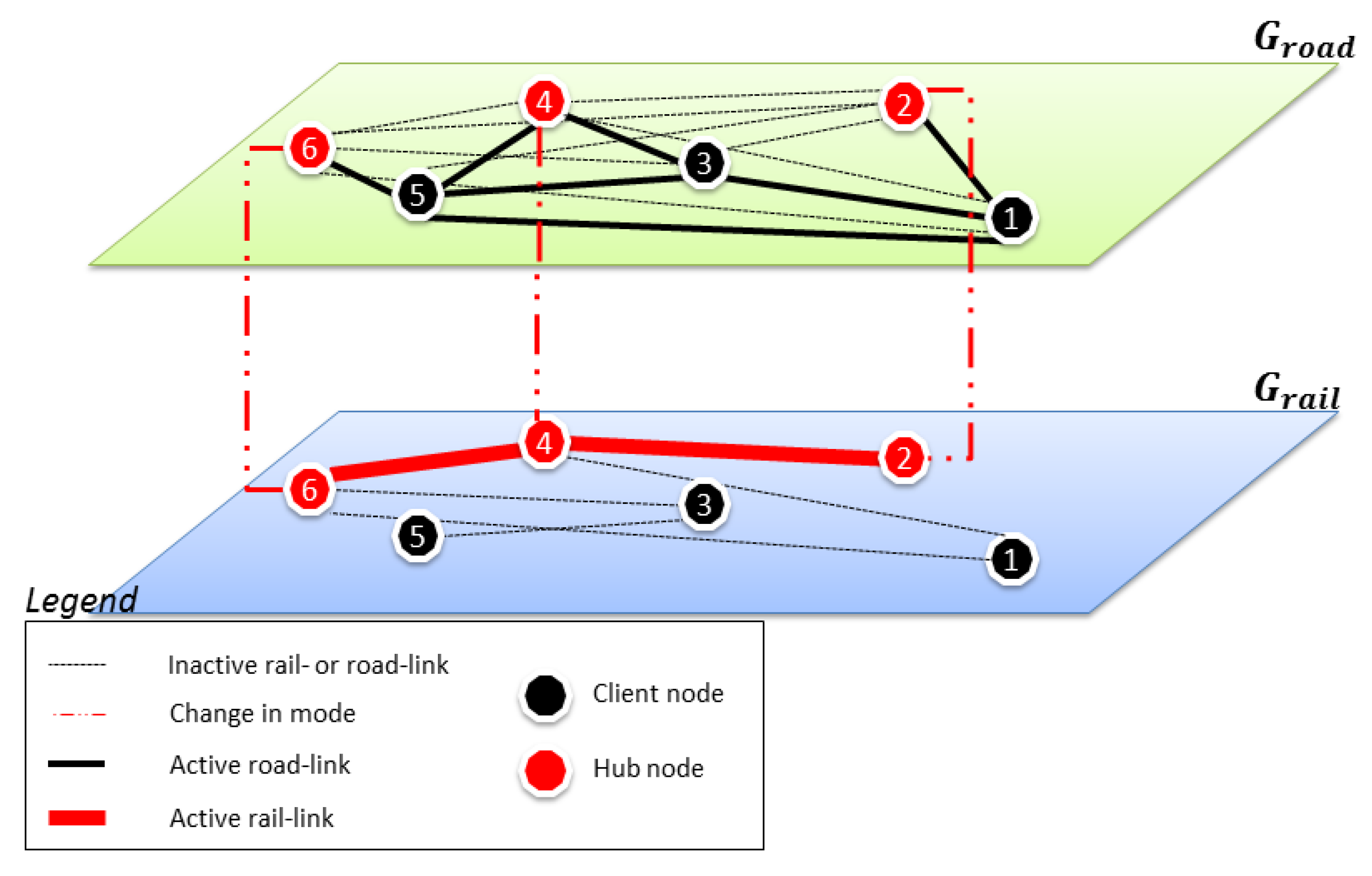
3.1. Problem Description

We model the intermodal green p-hub median problem as an incomplete graph $G=\{N,A\}$, where N is the set of all nodes in an instance. We denote $H\subset N$ the subset of potential rail terminals or hubs. For a solution, $A=A_{rail}\cup A_{road}$ represents the set of all active arcs between node pairs, and we enumerate $A_{rail}=\{(k,m)/k,m\in H\}$ the set of active rail-links and $A_{road}=A_{road}^{direct}\cup A_{road}^{hub}$ the set of active road-links. Where $A_{road}^{direct}=\{(i,j)/i,j\in N\}$ and $A_{road}^{hub}=\{(i,k),(k,i)/i\in N\backslash H,k\in H\}$ are the set of direct road-links between any two nodes and the set of direct client-hub and hub-client road-links, respectively.

When $q<\left(\frac{p(p-1)}{2}\right)$ the number of active direct rail-links, set $A_{rail}$ of rail-link between hub nodes constitutes an incomplete rail sub-graph $G_{rail}=\{H,A_{rail}\}$. In fact, real world rail freight transport networks remain incomplete, and most rail terminals are often only connected through a number of intermediate facilities. Whereas, the road sub-graph $G_{road}=\{N,A_{road}\}$ is assumed to be complete as any node pairs may be potentially reached through the road network. Nonetheless, road freight transport naturally incurs more CO${}_2$ emissions, and often comes at the cost of congestion. We mention that an example solution for a small instance is presented in Figure 1.

Figure 1. Graphical representation of opt solution for instance with $\left|N\right|=\left|H\right|=6$, $p=3$ and $q=2$.

In hub-networks, the number of access arcs to hub facilities increases with the number of allocated client nodes. Additionally, we consider that hub nodes act as rail terminals, where demand flows from various origins to many destinations are routed on-road by heavy-duty vehicles, then consolidated into freight trains in incomplete hub rail-networks.

For each open hub nodes $k,m\in H$, we assume that the consolidated demand flows may be transferred via one active rail-link from origin-hub to destination-hub, or via two active rail-links with an intermediate hub node $l\in H$. And we consider decision variables $z_{km}$ and $L_{km}^l$ to model the active direct and intermediate rail-links between hub pairs, respectively.

Variables $x_{ij}$, $f_{ij}^{km}$ and $y_{ij}^{lkm}$ are considered to represent if demand flows are sent directly on-road $A_{road}^{direct}$, directly between two hub nodes or through another intermediate facility in the road-rail network $A_{rail}\cup A_{road}^{hub}$, respectively. And we mention that the single-allocation scheme is assumed , thus a client node may only be allocated to one hub node. Nonetheless, direct on-road transport between hub and spoke pairs is allowed regardless of the allocation decision. For any origin-destination pairs, CO${}_2$ emission costs are incurred through the routing of the necessary demand flows in the road-rail hub-network. We note $E{C}_{ij}$ the on-road estimated CO${}_2$ emission costs for truck carrying demand flows directly from origin $i\in N$ to destination $j\in N$ ($x_{ij}=1$). Whereas, $HE{C}_{ij}^{km}$ and $LE{C}_{ij}^{lkm}$ represent the estimated CO${}_2$ emission costs of routing demand flows through the road-rail network when $f_{ij}^{km}=1$ or $y_{ij}^{lkm}=1$, respectively.

In Appendix A, we describe the mesoscopic road-emission model considered to estimate the CO₂ emission costs of vehicles travelling directly on-road $A_{road}^{direct}\cup A_{road}^{hub}$. We also present the mesoscopic rail-emission estimation model to estimate the CO${}_2$ emissions costs incurred through the transfer of consolidated flows in the incomplete rail network $A_{rail}$.

To formulate the intermodal green p-hub median problem with incomplete hub-network, we consider the following assumptions:

• Direct-links between spoke nodes are allowed.
• Demand flows are transferred on-rail between located hub nodes.
• All transportation on spoke-hub, hub-spoke and spoke-spoke direct links is performed on-road.
• In a solution, each spoke node i is allocated to only one hub node k. Nonetheless, direct on-road transportation between i and a hub node $m\ne k$ is allowed.
• Hub-networks are incomplete and at most one hub node $l\in H$ can be visited on the route between hub nodes $k\in H\backslash \left\{l\right\}$ and $m\in H\backslash \{l,k\}$.
• For any $(i,j)\in N$ origin-destination pair, $W_{ij}$ demand flows are sent either directly from i to j, directly on hub-link $z_{km}$ between hub nodes k and m, or through one intermediate hub-link $L_{km}^l$ with at most one hub $l\in H\backslash \{k,m\}$.

3.2. Mathematical Formulation

From the previously introduced notations (see Table 2 and Table 3 and assumptions, the intermodal green p-hub median problem with incomplete hub-network can be formulated as follows.

Table 2. Model Decision Variable Notations.

Decision Variables
$h_{ik}$	Binary variable equal to 1 if node $i\in N$ is allocated to hub node $k\in H$, 0 otherwise.
$z_{km}$	Binary variable equal to 1 if a rail-link between hub nodes $k,m\in H$ is active, 0 otherwise.
$L_{km}^l$	Binary variable that takes value 1 only if hub nodes $k,m\in H$ are connected through active intermediate rail-links with hub node $l\in H$.
$x_{ij}$	Binary variable equal to 1 if demand flows are routed on-road directly from node $i\in N$ to node $j\in N$, 0 otherwise.
$f_{ij}^{km}$	Binary variable equal to 1 only if demand flows are routed on-road from node $i\in N$ to hub node $k\in H$, directly on rail-link between hub nodes $k,m\in H$, then on-road from hub node $m\in H$ to node $j\in N$.
$y_{ij}^{lkm}$	Binary variable equal to 1 only if demand flows are routed on-road from node $i\in N$ to hub node $k\in H$, between hub nodes $k,m\in H$ through rail-links with hub node $l\in H$, then on-road from hub node $m\in H$ to node $j\in N$.
Dependant Variables
$E{C}_{ij}$	The estimated emission costs when routing demand flows directly on-road from node $i\in N$ to node $j\in N$.
$HE{C}_{km}^{ij}$	The estimated emission costs when routing demand flows on road-rail network from node $i\in N$ to node $j\in N$, and directly on rail-link between hub nodes $k,m\in H$.
$LE{C}_{ij}^{lkm}$	The estimated emission costs when routing demand flows on road-rail network from node $i\in N$ to node $j\in N$, and between hub nodes $k,m\in H$ through rail-link with hub node $l\in H$.

Table 3. Model Parameter Notations.

Model Parameters
N	Set of all nodes
H	Set of potential terminals
R	Set of speed levels
$d_{ij}$	The distance between nodes $i\in N$ and $j\in N$
$W_{ij}$	The amount of demand flow to be routed from node $i\in N$ to node $j\in N$
p	The number of hubs to locate
q	the number of active rail-links
$C^{train}$	The maximum payload of Train transferring demand flows between hub nodes
$\alpha$	The inter-hub cost discount factor for travel on rail-links between open hub nodes
M	A large number
$O_i$	The total flow originated from the node i, ${\displaystyle O_i=\sum _{j\in N}{W}_{ij}}$
$D_i$	The total flow destined to the node i, ${\displaystyle D_i=\sum _{j\in N}{W}_{ji}}$

• Hub location-allocation:

$$\begin{array}{c}\sum _{k\in H}{z}_{kk}=p\end{array}$$

(1)

$$\begin{array}{c}{z}_{km}\le z_{kk}\forall k,m\in H\end{array}$$

(2)

$$\begin{array}{c}{z}_{km}\le z_{mm}\forall k,m\in H\end{array}$$

(3)

$$\begin{array}{c}{L}_{km}^l\ge z_{kl}+z_{lm}-1-z_{km}\forall k,m,l\in H\end{array}$$

(4)

$$\begin{array}{c}{L}_{km}^l\le z_{kl}\forall k,m,l\in H\end{array}$$

(5)

$$\begin{array}{c}{L}_{km}^l\le z_{lm}\forall k,m,l\in H\end{array}$$

(6)

$$\begin{array}{c}{L}_{km}^l\le 1-z_{km}\forall k,m,l\in H\end{array}$$

(7)

$$\begin{array}{c}{z}_{km}=z_{mk}\forall k,m\in H\end{array}$$

(8)

$$\begin{array}{c}{L}_{km}^l=L_{mk}^l\forall k,m,l\in H\end{array}$$

(9)

$$\begin{array}{c}{h}_{ik}\le z_{kk}\forall i\in N,\forall k\in H,k\ne i\end{array}$$

(10)

$$\begin{array}{c}\sum _{i\in N,i\ne k}{h}_{ik}\ge z_{kk}\forall k\in H\end{array}$$

(11)

$$\begin{array}{c}\sum _{k\in H,k\ne i}{h}_{ik}=1-z_{ii}\forall i\in N\end{array}$$

(12)

$$\begin{array}{c}\sum _{m\in H,m\ne k}{z}_{km}\ge z_{kk}\forall k\in H\end{array}$$

(13)

$$\begin{array}{c}{z}_{km}+\sum _{l\in H\backslash \{k,m\}}{L}_{km}^l\ge z_{kk}+z_{mm}-1\forall k,m\in H,m\ne k\end{array}$$

(14)

$$\begin{array}{c}\sum _{k,m\in H,m\ne k}{z}_{km}=2.q\end{array}$$

(15)

First, Constraint (1) states that p hub nodes are located. Constraints (2) and (3) allow a rail-link $(k,m)$ to be active only if node k and node m are open hub nodes, respectively. Following, Constraints (4)–(7) ensure that hub nodes $k\in H$ and $m\in H$ are only connected through hub node $l\in H$ if rail-links $\left\{\right(k,l),(l,k),(m,l),(l,m\left)\right\}$ are active, while direct rail-links between k and m are not. Constraints (8) and (9) ensure that direct and intermediate rail-links active from hub k to hub m are also active from hub m to hub k. Next, Constraints (10) permit the allocation of node $i\in N$ to hub node $k\in H$ only if it is open. Constraints (11) force at least one non-hub node $i\in N,i\ne k$ to be allocated to open hub node $k\in H$. And Constraints (12) define the single-allocation scheme. For each open hub node $k\in H$, Constraints (13) state that at least one rail-link $(k,m),m\in H\backslash \left\{k\right\}$ must be active. Whereas, Constraints (14) establish that open hub nodes $k\in H$ and $m\in H$ must be linked either directly through one active rail-link, or via two active rail-links with an intermediate hub node $l\in H$. Finally, Constraint (15) sets the number of active direct rail-links in the hub-network.

When $q<\left(\frac{p(p-1)}{2}\right)$, the rail-network between hub nodes is incomplete. To efficiently capture the partition of demand flows, we propose decision variables $x_{ij}$, $f_{ij}^{km}$ and $y_{ij}^{lkm}$ to model routing of demand flows between o-d pairs directly on-road, on road-rail with one rail-link, and on road-rail via two rail-links, respectively. The following constraints handle the routing of demand flows in the road-rail hub-network.

• Demand Flows Routing:

$$\begin{array}{c}\sum _{k,m\in H}{f}_{ij}^{km}{W}_{ij}+\sum _{k,m,l\in H}{y}_{ij}^{lkm}{W}_{ij}+x_{ij}{W}_{ij}=W_{ij}\forall i,j\in N\end{array}$$

(16)

$$\begin{array}{c}\sum _{i,j\in N}{f}_{ij}^{km}{W}_{ij}\le C^{train}{z}_{km}\forall k,m\in H\end{array}$$

(17)

$$\begin{array}{c}\sum _{i,j\in N}{y}_{ij}^{lkm}{W}_{ij}\le C^{train}{L}_{km}^l\forall k,m,l\in H\end{array}$$

(18)

$$\begin{array}{c}\sum _{j\in N,m\in H}{f}_{ij}^{km}{W}_{ij}+\sum _{j\in N,m\in H}{f}_{ji}^{mk}{W}_{ji}\le (O_i+D_i)h_{ik}\forall i\in N,\forall k\in H\end{array}$$

(19)

$$\begin{array}{c}\sum _{j\in N,m,l\in H}{y}_{ij}^{lkm}{W}_{ij}+\sum _{j\in N,m,l\in H}{y}_{ji}^{lmk}{W}_{ji}\le (O_i+D_i)h_{ik}\forall i\in N,\forall k\in H\end{array}$$

(20)

$$\begin{array}{c}{f}_{km}^{km}{W}_{km}\ge W_{km}{z}_{km}\forall k,m\in H,k\ne m\end{array}$$

(21)

$$\begin{array}{c}\sum _{l\in H\backslash \{k,m\}}{y}_{km}^{lkm}\ge z_{kk}+z_{mm}-1-z_{km}\forall k,m\in H,k\ne m\end{array}$$

(22)

$$\begin{array}{c}{y}_{km}^{lkm}\le W_{km}{L}_{km}^l\forall k,m,l\in H,k\ne m\ne l\end{array}$$

(23)

Constraints (16) ensure that the total demand flows between each o-d pairs is routed in the road-rail hub-network. Additionally, Constraints (17) and (18) guarantee that the train maximum payload may not be exceeded when transferring demand flows directly between hub nodes k and m, and through hub node l, respectively. Whereas, Constraints (19) and (20) define an upper bound on the total originated and destined flows of node $i\in N$ that are routed by hub node $k\in H$. Furthermore, Constraints (21)–(23) force demand flows between open hub nodes to be transferred using the incomplete rail hub-network.

From the introduced parameter notations (see Table A1) and expressions (see Appendix A), the mesoscopic model [36] can be used to estimate the fuel consumption in $\left(L\right)$, respectively, for diesel trucks traveling on road or trains carrying consolidated demand flows through the rail hub-network.

• Emission costs estimation:

$$\begin{array}{c}\hfill E{C}_{ij}=e\left(\lambda \left(\left(\frac{d_{ij}}{v^{truck}}\right)(r^{idle}{x}_{ij}+{\beta }^{truck}{\chi }_{ij})\right)\right)+e\left(\lambda \left({\beta }^{truck}\left(n^{acc}{\pi }_{ij}{W}_{inert}^{truck}{d}_{ij}\right)\right)\right)\\ \hfill \forall i,j\in N,i\ne j\end{array}$$

(24)

$$\begin{array}{c}where,\\ {\pi }_{ij}=m^{truck}{x}_{ij}+x_{ij}{W}_{ij}\\ {\chi }_{ij}=P_{roll}^{truck}{\pi }_{ij}+P_{air}^{truck}{x}_{ij}\end{array}$$

Constraints (24) define the on-road total CO${}_2$ emission costs of vehicle transporting demand flows $W_{ij}$ directly from node $i\in N$ to node $j\in N$ when direct-link $x_{ij}$ is selected.

$$\begin{array}{c}HE{C}_{ij}^{km}=e\left(\lambda \left(\left(\frac{d_{ik}}{v^{truck}}\right)(r^{idle}{f}_{ij}^{km}+{\beta }^{truck}{\psi }_{ij}^{km})\right)\right)\\ +e\left(\lambda \left(\left(\frac{d_{mj}}{v^{truck}}\right)(r^{idle}{f}_{ij}^{km}+{\beta }^{truck}{\psi }_{ij}^{km})\right)\right)+e\left(\lambda \left({\beta }^{truck}\left(n^{acc}{\mu }_{ij}^{km}{W}_{inert}^{truck}(d_{ik}+d_{mj})\right)\right)\right)\\ \forall i\in N\backslash \{j,m\},\forall j\in N\backslash \{i,k\},\forall k,m\in H,k\ne m\end{array}$$

(25)

$$\begin{array}{c}LE{C}_{ij}^{lkm}=e\left(\lambda \left(\left(\frac{d_{ik}}{v^{truck}}\right)(r^{idle}{y}_{ij}^{lkm}+{\beta }^{truck}{\tilde{\psi }}_{ij}^{lkm})\right)\right)\\ +e\left(\lambda \left(\left(\frac{d_{mj}}{v^{truck}}\right)(r^{idle}{y}_{ij}^{lkm}+{\beta }^{truck}{\tilde{\psi }}_{ij}^{lkm})\right)\right)+e\left(\lambda \left({\beta }^{truck}\left(n^{acc}{\tilde{\mu }}_{ij}^{lkm}{W}_{inert}^{truck}(d_{ik}+d_{mj})\right)\right)\right)\\ \forall i\in N\backslash \{j,m,l\},j\in N\backslash \{i,k,l\},\forall k,m,l\in H,k\ne m,k\ne l,m\ne l\end{array}$$

(26)

$$\begin{array}{c}where,\\ {\mu }_{ij}^{km}=m^{truck}{f}_{ij}^{km}+f_{ij}^{km}{W}_{ij},{\tilde{\mu }}_{ij}^{lkm}=m^{truck}{y}_{ij}^{lkm}+y_{ij}^{lkm}{W}_{ij}\\ {\psi }_{ij}^{km}=P_{roll}^{truck}{\mu }_{ij}^{km}+P_{air}^{truck}{f}_{ij}^{km},{\tilde{\psi }}_{ij}^{lkm}=P_{roll}^{truck}{\tilde{\mu }}_{ij}^{lkm}+P_{air}^{truck}{y}_{ij}^{lkm}\end{array}$$

Similarly, The CO${}_2$ emission costs of vehicles supplying hub node $k\in H$ from origin $i\in N$ and delivering from hub node $m\in H$ to destination $j\in N$, respectively, are given by Constraints (25). When hub node $l\in H$ is visited by train traveling from hub $k\in H$ to hub $m\in H$, Constraints (26) determine the on-road CO${}_2$ emission costs of vehicles leaving origin i to hub k and reaching destination j from hub m, respectively.

$$\begin{array}{c}HE{C}_{km}^{km}=e\left(\lambda \left({\beta }_{diesel}^{train}\left(\left(\frac{d_{km}}{v^{train}}\right){\phi }^{km}\right)\right)\right)+e\left(\lambda \left({\beta }_{diesel}^{train}\left(n^{acc}{M}^{km}{W}_{inert}^{train}{d}_{km}\right)\right)\right)\\ +{\displaystyle \sum _{i\in N\backslash \{j,m\},j\in N\backslash \{i,k\}}}HE{C}_{ij}^{km}\forall k,m\in H,k\ne m\end{array}$$

(27)

$$\begin{array}{c}LE{C}_{km}^{lkm}=e\left(\lambda \left({\beta }_{diesel}^{train}\left(\left(\frac{(d_{kl}+d_{lm})}{v^{train}}\right){\tilde{\phi }}^{lkm}\right)\right)\right)\\ +e\left(\lambda \left({\beta }_{diesel}^{train}\left(n^{acc}{\tilde{M}}^{lkm}{W}_{inert}^{train}(d_{kl}+d_{lm})\right)\right)\right)+{\displaystyle \sum _{i\in N\backslash \{j,m,l\},j\in N\backslash \{i,k,l\}}}LE{C}_{ij}^{lkm}\\ \forall k,m,l\in H,k\ne m,k\ne l,m\ne l\end{array}$$

(28)

$$\begin{array}{c}where,\\ M^{km}=m^{train}{f}_{km}^{km}+\sum _{i,j\in N}{f}_{ij}^{km}{W}_{ij},{\tilde{M}}^{lkm}=m^{train}{y}_{km}^{lkm}+\sum _{i,j\in N}{y}_{ij}^{lkm}{W}_{ij}\\ P_{roll}^{cte}=P_{roll}^{Loc}+P_{roll}^{Car}+P_{roll}^{Axles},P_{roll}^{Aux}=P_{roll}^{Aux1}+P_{roll}^{Aux2}\\ {\phi }^{km}=P_{air}^{train}{f}_{km}^{km}+P_{roll}^{cte}{f}_{km}^{km}+P_{roll}^{Aux}{M}^{km},{\tilde{\phi }}^{lkm}=P_{air}^{train}{y}_{km}^{lkm}+P_{roll}^{cte}{y}_{km}^{lkm}+P_{roll}^{Aux}{\tilde{M}}^{lkm}\end{array}$$

Constraints (27) compute the total CO${}_2$ emission costs for diesel train transferring consolidated demand flows directly from hub $k\in H$ to hub $m\in H$. Whereas, Constraints (28) compute the total CO${}_2$ emission costs to transfer consolidated flows from hub $k\in H$ to hub $m\in N$ and visiting hub $l\in H$ on its route.

Furthermore, we note that trucks may perform additional hub-spoke, (or spoke-hub) and spoke-spoke trips transporting demand flows directly from (or to) a hub node to (or from) one of its allocated client nodes, or between client nodes visiting one and only one hub node on the route, respectively. We propose Constraints (29)–(31) to compute the total CO${}_2$ emission costs incurred by the on-road transportation of demand flows within one hub node.

$$\begin{array}{c}\hfill HE{C}_{ki}^{kk}=e\left(\lambda \left(\left(\frac{d_{ki}}{v^{truck}}\right)(r^{idle}{f}_{ki}^{kk}+{\beta }^{truck}{\psi }_{ki}^{kk})\right)\right)+e\left(\lambda \left({\beta }^{truck}\left(n^{acc}{\mu }_{ki}^{kk}{W}_{inert}^{truck}{d}_{ki}\right)\right)\right)\\ \hfill \forall i\in N,\forall k\in H,k\ne i\end{array}$$

(29)

$$\begin{array}{c}\hfill HE{C}_{ik}^{kk}=e\left(\lambda \left(\left(\frac{d_{ik}}{v^{truck}}\right)(r^{idle}{f}_{ik}^{kk}+{\beta }^{truck}{\psi }_{ik}^{kk})\right)\right)+e\left(\lambda \left({\beta }^{truck}\left(n^{acc}{\mu }_{ik}^{kk}{W}_{inert}^{truck}{d}_{ik}\right)\right)\right)\\ \hfill \forall i\in N,\forall k\in H,k\ne i\end{array}$$

(30)

$$\begin{array}{c}HE{C}_{ij}^{kk}=e\left(\lambda \left(\left(\frac{(d_{ik}+d_{kj})}{v^{truck}}\right)(r^{idle}{f}_{ij}^{kk}+{\beta }^{truck}{\psi }_{ij}^{kk})\right)\right)\\ +e\left(\lambda \left({\beta }^{truck}\left(n^{acc}{\mu }_{ij}^{kk}{W}_{inert}^{truck}(d_{ik}+d_{kj})\right)\right)\right)\forall i\in N\backslash \{j,k\},\forall j\in N\backslash \{i,k\},\forall k\in H\end{array}$$

(31)

$$HE{C}_{kk}^{kk}=\sum _{i\in N\backslash \{j,k\},j\in N\backslash \{i,k\}}HE{C}_{ij}^{kk}+\sum _{i\in N,i\ne k}HE{C}_{ik}^{kk}+\sum _{j\in N,j\ne k}HE{C}_{kj}^{kk}\forall k\in H$$

(32)

Constraints (29) represent the total CO${}_2$ emission costs of transporting demand flows directly from hub node $k\in H$ to its client node $i\in N$. And, Constraints (30) establish the total CO${}_2$ emission costs of routing demand flows directly from client node $i\in N$ to its hub node $k\in H$. Whereas, Constraints (31) give the expression of the total CO${}_2$ emission costs of trucks carrying demand flows from origin $i\in N$ to hub node $k\in H$, then from hub node $k\in H$ to destination $j\in N$. Constraints (32) are the sum of CO${}_2$ emission costs incurred by on-road transport within one hub node.

• Objective cost:

$$\begin{array}{c}Min\sum _{i,j\in N}E{C}_{ij}+\sum _{k,m\in H}HE{C}_{km}^{km}+\sum _{k,m,l\in H}LE{C}_{km}^{lkm}\end{array}$$

(33)

The objective of our formulation is to minimize the total CO${}_2$ emission costs incurred through the transport of all necessary demand flows in the road-rail hub network.

4. Genetic Algorithm

The problem formulated in Section 3 retains the properties of the p-hub median problem (p-HMP), integrates transportation-based CO${}_2$ emission costs in the model, and extends the location decision to the selection of intermodal terminals (i.e., hubs) such as demand flows are routed in incomplete hub-networks. In the literature, the p-HMP and the intermodal hub location problem (IHLP) are both known to be NP-Hard, which makes the intermodal green p-hub median problem with incomplete hub-network (I-Gp-IHMP) also NP-Hard. Thus, large sized instances may not be solved using exact methods. Whereas heuristic or meta-heuristic methods may be considered to offer good solutions in reasonable runtimes.

GA was first described by J.H Holland in 1960, and developed jointly with a team in the University of Michigan. In [37], the author introduced a theoretical framework for GA implementation. The method is inspired from the theory of natural evolution proposed by Charles Darwin. Thus, the fittest individuals in the population is preserved during the search process. Initially, a population of individual is generated. Then until a stopping criterion is met, the population-based search heuristic selects a pair of parent individuals and applies cross-over and mutation operators to produce new off-springs. Also, solution encoding or representation and individual evaluation function play a key role in the adaptation of genetic algorithms.

To solve the I-Gp-IHMP, we propose a genetic algorithm with value-encoding individuals, and a best path construction heuristic to initialize the population. Additionally, novel cross-over and mutation operators are implemented to search for better off-springs. The rank selection method is considered to select parents for cross-over. Furthermore, we mention that a new parent is selected from the population for mutation. In contrast, traditional GA implementations often allow mutation to occur only on newly generated off-springs through cross-over. Finally, demand flows routing heuristic is developed to efficiently determine the partition of demand flows in the incomplete road-rail network.

The general framework of our GA is given in Algorithm 1. And we describe our solution approach in following sections as follows. in Section 4.1, we present the solution encoding and individual fitness function. The new best path heuristic considered to generate initial individuals is described in Section 4.2. Whereas, the novel demand flows routing heuristic as well as cross-over and mutation operators can be found in Section 4.3 and Section 4.4, respectively.

Algorithm 1: Genetic Algorithm.

4.1. Solution Encoding and Fitness Function

The first step in a genetic algorithm is to model any solution (i.e., individual) as chromosomes. A chromosome is a sequence of genes representing any individual in the population. And each gene may take specific values depending on the encoding scheme. In the literature, many encoding schemes (Binary, Permutation, Value, Tree, etc.) were proposed to offer more suitable chromosomes representation.

For our particular problem, An individual is a solution X to the following three sub-problems: (i) the location of p hub nodes in a rail-network with q direct-links, (ii) The allocation of all non-hub nodes to located hub nodes, and (iii) the partition of the demand flows in the incomplete hub network. Whereas, the fitness of a solution is represented by the total transportation-based CO${}_2$ emission costs of required demand flows through the incomplete road-rail network. A solution is deemed infeasible if it violates the train maximum payload $C^{train}$ on any arc $(k,m)\in A^{rail}$. And we mention that a penalty cost $penalty(\varrho ,X)$ is imposed to degrade the fitness of infeasible individuals, where $\varrho$ is a penalty parameter. Thus, decreasing their chances of survival in the next generations. Nonetheless, these individuals may still be selected to maintain diversity during the search phase of our algorithm.

In our GA, value encoding was considered to determine the respective genes in the chromosomes representation. For each individual X, vector $R\left(X\right)$ and vectors $A^k\left(X\right)$ represent the incomplete rail-network with p located hub nodes $k\in H$, and the allocation of client nodes to each open hub k, respectively. Thus, fitness $F\left(X\right)$ of individuals could be computed directly and without unnecessary value conversion of each gene as follows:

$$\begin{array}{c}F\left(X\right)=obj\left(X\right)+penalty(\varrho ,X),\mathrm{where}\\ penalty(\varrho ,X)=\varrho \underset{k,m\in R\left(X\right)}{max}(0,\sum _{i,j\in A^k\left(X\right)\cup A^m\left(X\right)}{f}_{ij}^{km}-C^{train})\\ +\varrho \underset{l,k,m\in R\left(X\right)}{max}(0,\sum _{i,j\in A^k\left(X\right)\cup A^m\left(X\right)}{y}_{ij}^{lkm}-C^{train})\end{array}$$

We note $obj\left(X\right)$ the total estimated CO${}_2$ emission costs as given in Equation (33). Whereas, we present in Figure 2 an example of our GA solution encoding where rail network and allocation-list denote vector $R\left(X\right)$ and vectors $A^k\left(X\right)$, respectively. Additionally, the demand flows routing heuristic (see Section 4.3) could be considered to handle the partition of demand flows in the incomplete road-rail hub-network. Then, the CO${}_2$ emission costs could be easily estimated using models presented in Appendix A, and fitness $F\left(X\right)$ may be dynamically updated.

Figure 2. Genetic algorithm solution encoding example for instance with $\left|N\right|=\left|H\right|=10$, $p=3$ and $q=2$.

4.2. GA Initial Population

To initialize our GA, each individual in the population will be generated using a novel heuristic approach. Then, its respective fitness $F\left(X\right)$ will be set as described in Section 4.1. We propose a best-path construction heuristic (BP-CH) to offer good quality solutions for the initial population. For diversification, we mention that one open hub node will also be randomly selected at each time for each individual. Specifically, our BP-CH will proceed as follows.

First, one potential hub node $hu{b}_1\in H$ is selected randomly and opened. Following, we initialize $PHub{s}^k$ the sets representing the distinct union of potential hubs $Phu{b}_2,Phu{b}_3,\dots ,Phu{b}_p\in H\backslash \left\{hu{b}_1\right\}$ with previously located hub $hu{b}_1$. Then, we compute ${\delta }^{PHub{s}^k}$ the distance cost for each path between hubs in set $PHub{s}^k$ as follows:

$$\begin{array}{c}{\delta }^{PHub{s}^k}=d_{Phu{b}_2;hu{b}_1}+d_{Phu{b}_2;Phu{b}_3}+\dots +d_{Phu{b}_2;Phu{b}_p},where\\ PHub{s}^k=\{hu{b}_1,Phu{b}_2,Phu{b}_3,\dots ,Phu{b}_p\}\end{array}$$

The best path is identified as the minimum cost ${\delta }^{PHub{s}^k}$ achieved by a potential link-hub node $Phu{b}_2$ in set $PHub{s}^k$. And a link-hub node is defined as a hub from which all other hub nodes can be reached directly. hub nodes $hu{b}_i$ are then located such as $Hubs=PHub{s}^k$ with $PHub{s}^k$ is set of potential terminals verifying $min({\delta }^{PHub{s}^k})$. And all direct-links between link-hub $hu{b}_2\in Hubs$ and remaining hub nodes $hub\in Hubs\backslash \left\{hu{b}_2\right\}$ are activated to setup the incomplete hub-network. Algorithm 2 describes the best path search heuristic for a randomly selected hub $hu{b}_1\in H$.

At this step, p hub nodes are located in an incomplete rail-network. Next, our construction heuristic will attempt to allocate each non-hub node to only one located hub in $Hubs$. For on road- and rail-transport, we know that the total CO${}_2$ emission costs (i.e., the objective cost) shows a positive correlation with the traveled distance and the carried load between each o-d pairs. Thus, we propose a distance-based priority allocation heuristic to offer good initial individuals.

Algorithm 2: best Path Search Heuristic

Initially, a $client\in N\backslash Hubs$ will only be allocated to $hu{b}_i\in Hubs$ when it is the closest located hub to $client$, and $hu{b}_i$ has no other allocated clients. Then, once p client nodes are allocated, remaining nodes are simply each allocated to their nearest hub node $hu{b}_i\in Hubs$ in terms of distance cost. The priority allocation heuristic is presented in Algorithm 3.

Algorithm 3: Priority Allocation Heuristic

To conclude, the best path construction heuristic is considered to locate p hub nodes in an incomplete rail-network, and allocate the remaining nodes to open hubs with a distance-based priority allocation heuristic. Effectively answering the first two sub-problems (see Section 4.1) for a solution of our GA. Nonetheless, the partition of demand flows in the road-rail network needs to be decided to estimate the CO${}_2$ emission costs, and evaluate each solution. In the next section, we present the demand flows routing heuristic considered to solve the third sub-problem and compute the fitness of individuals in our GA.

4.3. Demand Flows Routing Heuristic

In the previous sections, we have introduced the encoding scheme and the heuristic approach considered to generate initial individuals for our population based meta-heuristic. For a given $R\left(X\right)$ and $A^1\left(X\right),A^2\left(X\right),\dots ,A^p\left(X\right)$, we have also established that solving the demand flows routing problem was required to evaluate any individual X, and compute fitness $F\left(X\right)$. For this purpose, our proposed heuristic will initially compute the total CO${}_2$ emission costs such as all demand flows are transferred through the incomplete hub-network. Then, improvement procedures will at each step reverse the demand flows to direct on-road transport.

Initially, we set $f_{ij}^{kk}=1$, $f_{ij}^{km}=1$ and $y_{ij}^{lkm}=1$ for all $i,j\in N\backslash Hubs$ client nodes allocated to one hub node $k\in Hubs$, to hub nodes $k,m\in Hubs$ via one direct rail-link and via two rail-links with hub node $l\in Hubs$, respectively. Additionally, we initialize demand flows $f_{ki}^{kk}=1$ and $f_{ik}^{kk}=1$ for all hub-client and client-hub arcs between client nodes $i\in N\backslash Hubs$ allocated to hub $k\in Hubs$. And For each hub nodes $k,m\in Hubs$, $f_{kj}^{km}=1$ (resp. $\left(f_{im}^{km}=1\right)$) and $y_{kj}^{lkm}=1$ (resp. $\left(y_{im}^{lkm}=1\right)$) demand flows from each hub k to clients j allocated to each hub m (resp. to each hub m from clients i allocated to hub k) when $z_{km}=1$ and when $L_{km}^l=1$. Furthermore, the total demand flows transferred on hub arcs $(k,m)\in A^{rail}$ are set to estimate $HE{C}_{km}^{km}$ and $LE{C}_{km}^{lkm}$, and compute the objective cost of solution X as follows.

$${\displaystyle F\left(X\right)=\sum _{k,m\in Hubs}HE{C}_{km}^{km}+\sum _{k,m,l\in Hubs}LE{C}_{km}^{lkm}}$$

Following, for each $f_{ij}^{kk}=1$, direct on-road $x_{ij}=1$ demand flows are set on arc $(i,j)$ only when $d_{ij}<(d_{ik}+d_{kj})$. Then, for each $f_{ij}^{km}$, we compute $\Delta F\left(X\right)$ the variation in the objective cost when $x_{ij}=1$ and $f_{ij}^{km}=0$.

$$\Delta F\left(X\right)=F\left(X\right)-\tilde{F}\left(X\right), \mathrm{where} \tilde{F}\left(X\right)=F\left(X\right)-(HE{C}_{ij}^{km}+HE{C}_{km}^{km})+(E{C}_{ij}+{\widetilde{HEC}}_{km}^{km})$$

When $\Delta F\left(X\right)>0$, the demand flows transferred between hub nodes are reversed to direct on-road transportation. Similarly, for each $f_{kj}^{km},f_{im}^{km},y_{ij}^{lkm},y_{kj}^{lkm},y_{im}^{lkm}=1$, this procedure is repeated and direct on-road demand flows are set when better costs are identified.

The demand flows routing heuristic stops when all new $(i,j)$ direct on-road arcs necessarily degrade the objective cost, thus efficiently answering the last sub-problem. Should solution X be infeasible, a capacity repair procedure is considered until X is feasible or until at most $c_{repair}$ repairs are performed, such as one flow sent on rail-link with capacity violation is randomly selected and switched to direct on-road transport between o-d pairs. Then, a penalty cost (see Section 4.1) is added to fitness $F\left(X\right)$ of any infeasible individual X.

4.4. Crossover and Mutation Operators

During the search phase, our GA attempts to evade premature convergence to local minimums through the selection of individuals for both cross-over and mutation. At each time, a new off-spring $X_{child}$ will be introduced in the population by applying only one cross-over or mutation operator as described in Table 4.

Table 4. Cross -over and Mutation Operators.

Cross-over operators
Mutual Exchange	For selected parents $X_1$ and $X_2$, produce new off-spring $X_{child}$ such as $R\left(X_{child}\right)=R\left(X_1\right)$ and $A^k\left(X_{child}\right)=A^k\left(X_2\right),\forall k\le p$.
Link-Hub Exchange	For selected parents $X_1$ and $X_2$, produce new off-spring $X_{child}$ such as $R\left(X_{child}\right)=R\left(X_1\right)$ and $A^k\left(X_{child}\right)=A^k\left(X_1\right),\forall k\le p$. Then, exchange link-hub in $R\left(X_{child}\right)$ with link-hub in $R\left(X_2\right)$
Non Link-Hub Exchange	For selected parents $X_1$ and $X_2$, produce new off-spring $X_{child}$ such as $R\left(X_{child}\right)=R\left(X_1\right)$ and $A^k\left(X_{child}\right)=A^k\left(X_1\right),\forall k\le p$. Then, exchange one non-link hub in $R\left(X_{child}\right)$ with one non-link hub in $R\left(X_2\right)$.
Mutation operators
Link-Hub Change	For selected individual X, produce new off-spring $X_{child}$ such as $R\left(X_{child}\right)=R\left(X\right)$ and $A^k\left(X_{child}\right)=A^k\left(X\right),\forall k\le p$. Then, select one client node in $A^k\left(X_{child}\right)$ and replace link-hub node in $R\left(X_{child}\right)$.
Non Link-Hub Change	For selected individual X, produce new off-spring $X_{child}$ such as $R\left(X_{child}\right)=R\left(X\right)$ and $A^k\left(X_{child}\right)=A^k\left(X\right),\forall k\le p$. Then, select one client node in $A^k\left(X_{child}\right)$ and replace one non link-hub node in $R\left(X_{child}\right)$.
Link-Hub Swap	For selected individual X, produce new off-spring $X_{child}$ such as $R\left(X_{child}\right)=R\left(X\right)$ and $A^k\left(X_{child}\right)=A^k\left(X\right),\forall k\le p$. Then, select one non link-hub in $R\left(X_{child}\right)$ and replace link-hub node in $R\left(X_{child}\right)$.
Non-Link Hub Swap	For selected individual X, produce new off-spring $X_{child}$ such as $R\left(X_{child}\right)=R\left(X\right)$ and $A^k\left(X_{child}\right)=A^k\left(X\right),\forall k\le p$. Then, select two non link-hubs in $R\left(X_{child}\right)$ and swap all their respective client nodes.
Reallocate Client	For selected individual X, produce new off-spring $X_{child}$ such as $R\left(X_{child}\right)=R\left(X\right)$ and $A^k\left(X_{child}\right)=A^k\left(X\right),\forall k\le p$. Then, select one client node in $A^k\left(X_{child}\right)$ and allocate it to a different open hub.
Swap Clients	For selected individual X, produce new off-spring $X_{child}$ such as $R\left(X_{child}\right)=R\left(X\right)$ and $A^k\left(X_{child}\right)=A^k\left(X\right),\forall k\le p$. Then, swap two client nodes in $A^k\left(X_{child}\right)$ each allocated to a different hub.

Additionally, we mention that specific repair procedures were required to fix each new off-spring $X_{child}$, and produce appropriate vectors $R\left(X_{child}\right)$ and $A^1\left(X_{child}\right),A^2\left(X_{child}\right),\dots$$,A^p\left(X_{child}\right)$. For example, when mutual exchange operator is run for selected parents $X_1$ and $X_2$, hub nodes in parent $X_1$ may be client nodes in parent $X_2$. Thus, the allocation vectors of new child individual must be repaired such as one hub $\left(hu{b}_{X_1}\in R\left(X_1\right),hu{b}_{X_1}\notin R\left(X_2\right)\right)$ is selected at each time to replace one hub $\left(hu{b}_{X_2}\in R\left(X_2\right),hu{b}_{X_2}\notin R\left(X_1\right)\right)$, if it is also allocated as a client node in off-spring $X_{child}$.

Furthermore, the demand flows routing heuristic is run for $X_{child}$ (see Section 4.3), and fitness $F\left(X_{child}\right)$ is computed. Then, a new cross-over and mutation operator is selected and run when cross-over and mutation probabilities are met, respectively. And when the initial population has been updated for a predefined number of generations, our GA terminates and returns the individual with best fitness value.

To summarize, we have introduced a genetic algorithm to solve the intermodal green p-hub median problem with incomplete hub-network. For each individual, a new best path construction heuristic was considered to initialize location an allocation vectors with regards to the solution encoding scheme. Then, a demand flows routing heuristic was used to efficiently compute the fitness cost. Whereas, novel cross-over and mutation operators were implemented to produce new off-springs.

5. Computational Experiments

In this section, we present the results of extensive computational experiments on the intermodal green p-hub median problem with incomplete hub-network. A comparison study between solutions returned by CPLEX and our GA can be found in Section 5.2. Following, we perform a comparison study between the road-rail and the road only hub-spoke networks in terms of the CO${}_2$ emission costs, and discuss the tuning of freight trains in Section 5.3. Then, Section 5.4 is reserved for a study of the robustness of the proposed solution approach.

Additionally, We mention that all algorithms are implemented in JAVA programming language and run on our PC with an Intel i7-7500 with up to 2.90 GHz. Whereas, all instances solved using the IBM commercial solver CPLEX are run for a maximum time limit of two hours, and with a maximum tree-size of 10 GB. Relevant data for distance and demand flows matrices are found in [4] datasets. Also, $\alpha =0.5$ inter-hub discount factor for travel using rail-links was set in all following results.

Furthermore, we performed extensive computational tests to set values for parameters of our GA. Various configurations ($GA(p,g,c,m)$) were considered to solve all instances solved optimally using CPLEX, where $p=\{50,100,250,500\}$, $g=\{500,1000,5000,10000\}$, $c=\{0.3,0.6,0.9\}$ and $m=\{0.3,0.6,0.9\}$ are the population size, the number of generations, the crossover-rate and the mutation-rate, respectively. We note that configuration with $GA(100,1000,0.3,0.3)$ was able to return all optimal solutions in competitive CPU times, thus we retain it for all computational experiments using our solution approach.

Table 5 regroups notations used in all computational tables, and the expression for each percentage gap notation is given as follows:

$$\begin{array}{c}\%Gap=\left(\frac{UB-LB}{UB}\times 100\right),\\ \%GapUB=\left(\frac{Obj-UB}{UB}\times 100\right),\\ \%GapLB=\left(\frac{Obj-LB}{Obj}\times 100\right),\\ \%GapRail=\left(\frac{Obj(Road/Rail)-Obj\left(Road\right)}{Obj\left(Road\right)}\times 100\right)\end{array}$$

Table 5. Computational Table Notations.

Notations
Obj		The objective cost of a solution as returned by our GA.
UB		The objective cost of the best upper bound found by CPLEX.
LB		The value of the lower bound found by CPLEX.
%Gap		The deviation in % for each instance between the UB and LB.
%GapUB		The deviation in % for each instance between the Obj and UB returned by our GA and CPLEX respectively.
%GapLB		The deviation in % for each instance between the Obj and LB returned by our SAA meta-heuristic and CPLEX respectively.
%GapRail		The deviation in % for each instance between the objective cost of the road-rail case and the objective cost of the road-only case.

5.1. Effect of the Heuristic Methods

In this section, we study the effect of the best-path construction heuristic (BP-CH) and the demand flows routing heuristic on the solutions obtained by our genetic algorithm. Our aim is to assess the performance of the implemented heuristics during the runs of our meta-heuristic, and to this end we develop two variants of our GA. In the first variants, the initial population will be generated using a random approach. Specifically, p hub nodes will be selected randomly from H the set of potential terminals at each time, and located as hub nodes. Following, the incomplete rail-network will be set such as one possible link is selected randomly at each time and activated. When q rail-links are active, each non-hub node is allocated randomly to a hub node, then the demand flows routing heuristic is run to compute the fitness of new individual. In the second variant, the location and allocation steps will be performed similarly to the first variant. Whereas, the demand flows routing heuristic will be replaced by a random routing approach during the generation of the initial population and of the off-springs.

In Table 6, we present the objective cost found by our GA, Variant one and two for selected instances with $\left|N\right|=\{10,20,40,50\}$, $p=\{3,5\}$ and heavy-freight trains. We note that both variants were unable to obtain optimal solutions for all smallest-sized instances with $\left|N\right|=10$, only Variant 1 was able to return the optimal solution for instance with $p=5$. Also, our BP-CH with demand flows routing heuristic outperforms the first and second variants for all remaining instances. $0.00$, $14.30$ and $4.98$ denote the best, the worst and the average $\%GapGA$ in the following order. Furthermore, the obtained results indicate that the first variant performs better than the one without the demand flows routing heuristic. Thus, in all following computational experiments, we retain the best-path construction heuristic and the demand flows routing heuristic during the run of our meta-heuristic.

Table 6. Objective cost comparison between our GA, Variant 1 and Variant 2.

			GA		Variant 1			Variant 2
|N|	p		Obj (£)		Obj (£)	%GapGA		Obj (£)	%GapGA
10	3		173.68		174.07	0.22		174.46	0.45
	5		369.28		369.28	0.00		369.56	0.07
20	3		643.84		656.26	1.93		691.10	7.34
	5		765.11		777.39	1.60		774.08	1.17
40	3		2377.43		2499.75	5.14		2546.11	7.09
	5		2458.93		2672.57	8.69		2810.61	14.30
50	3		3434.24		3614.85	5.26		3688.55	7.40
	5		3459.26		3743.21	8.21		3834.08	10.83

5.2. Comparison Study CPLEX and GA

Traditional formulations of the p-hub median problem are known to be NP-Hard. In our case, we also include the cost of transportation-based CO${}_2$ emissions into the model. Also, we assume that the rail hub-network is incomplete such as only a specific number q of direct rail-links are activated. In the following section, we solve small- and medium-sized [4] instances using the IBM commercial solver CPLEX as well as our own meta-heuristic. We show that CPLEX was unable to effectively solve all instances in the allotted runtime and tree-memory size. Whereas, all optimal solutions found by the exact method were returned using our GA in competitive CPU times.

Table A2, Table A3 and Table A4 in Appendix B report the results for the runs performed using both aforementioned methods, and when considering heavy-, medium- and light-freight trains, respectively. Initially, we see that the smallest sized instances ($\left|N\right|=10$) were able to be solved by CPLEX with a $\%Gap=0.00$. And we note $Avg\left(CP{U}^H\right)=10.624$ s, $Avg\left(CP{U}^M\right)=10.127$ s and $Avg\left(CP{U}^L\right)=12.482$ s the average time taken by the solver to return optimal solutions for heavy-, medium- and light-freight trains, respectively. For remaining instances, the exact method was unable to return integer solutions, especially due to memory requirements. Additionally, our GA is able to solve all considered instances in no more than $CPU\left(Worst\right)=13.50$ s (see instance with $\left|N\right|=20$, $p=5$ and $q=10$ with medium trains), and returns all optimal solutions in average runtimes $Avg\left(CP{U}_{G{A}^{OPT}}^H\right)=3.17$ s, $Avg\left(CP{U}_{G{A}^{OPT}}^M\right)=5.65$ s and $Avg\left(CP{U}_{G{A}^{OPT}}^L\right)=5.51$ s when heavy, medium and light freight trains are employed.

Furthermore, for all instances solved by CPLEX, we note that increasing the number of rail-links yields a decreasing improvement to the objective cost. Specifically, it seems that objective cost obtained for any instance with q rail-links is improved whenever one link is added until the network is complete. For example, we mention instance with $\left|N\right|=10$, $p=5$ for which increasing active rail-links one by one respectively improves the objective cost in percentage by $-6.88$, $-2.46$, $-2.12$, $-0.03$, $-0.02$, and $-0.01$ when considering heavy-trains. Figure 3 regroups all results for remaining settings. These results indicate that incomplete networks with a specific number of active rail-links may be preferable in real cases, especially since the gain from having a complete network does not seem to justify additional investment costs.

Figure 3. Variation in objective cost relative to number of rail-links.

5.3. Unimodal and Intermodal Transport for Complete and Incomplete Hub-Networks

In this section, we offer a comparison study between the traditional or unimodal green p-hub median problem and the intermodal case proposed in this work. We mention that [4] instances are solved using our GA for both complete and incomplete hub-networks. For the unimodal case, we assume that uncapacitated trucks are in charge of the transfer of consolidated flows between open hub nodes. Whereas, the capacity Constraints (17) and (18) are relaxed for the road-rail case. Similarly, we consider different settings (light, medium and heavy) for freight trains to compare the transportation-based CO${}_2$ emissions costs incurred through the intermodal and the unimodal distribution of required demand flows.

In Table A5 and Table A6 in Appendix B, we present the results of our GA respectively for the small- and medium-sized and for the large-sized [4] instances with incomplete hub-networks and heavy freight trains. We note that road transport appears to surpass road-rail transport for the smallest instances ($\left|N\right|\le 30$). For medium-sized instances, the road-rail model seems able to identify better cost solutions only when the number of open hubs does not exceed instance specific values ($p\le 5$ when $\left|N\right|=40$ and $p\le 6$ when $\left|N\right|=50$). Also, increasing the number of located hubs does not necessarily lead to solutions with better $\%GapRail$. Whereas, the unimodal case (e.g., on-road transport) appears to be better than the multi-modal (e.g., road-rail transport) case when $p=7$ for all considered small- and medium-sized instances. Furthermore and for all instances when $\%GapRail<0$, different hub nodes are located depending on the selected transport mode during hub transfers. For example, we mention instance ($\left|N\right|.p=50.3$) where nodes ($19,34,5$) are open hubs nodes for on-road transport, and where nodes ($4,39,25$) are established as intermodal hubs or rail terminals. Nonetheless, some nodes seem to be interesting hub candidates (e.g., node 33 for $\left|N\right|.p=40.3$), and thus are located in best found solutions of both the road and the road-rail case.

For all large-sized ($\left|N\right|\ge 70$) instances, the transfer of consolidated demand flows using incomplete rail-networks seems to significantly improve the total transportation-based CO${}_2$ emission costs. We note $Avg(\%GapRail)=5.76$ the average percentage gap between objective cost of all solutions of the unimodal and the multi-modal cases when hub-networks are incomplete. Additionally, solutions with better $\%GapRail$ were found for the largest sized instance with $\left|N\right|=200$, and the $\%GapRail$ appears to improve whenever more hub nodes are located. Whereas, the solution with best $\%GapRail$ was found when $p=6$ for the large-sized instance with $\left|N\right|=100$. For remaining instances, the decision on the number of open hubs also appears to be a necessary step to identify solutions with the best gap relative to on-road only transport. This indicates that a new mathematical formulation which considers the number of open hubs as a decision variable may be able to identify the optimal value p for each tackled instance. Similarly, we note that different hub nodes are open in BFS for same instances when considering either unimodal or intermodal transport, respectively.

Furthermore, we also compare the solutions obtained using our GA for the [4] instances when hub-networks are complete. For fixed number of open hubs, Figure A1, Figure A2 and Figure A3 show that unimodal transport by heavy-duty vehicles may still be preferred to intermodal transport by heavy-freight trains for small-sized instances ($\left|N\right|\le 30$). For medium-sized instances with $\left|N\right|=40$ and $\left|N\right|=50$, our GA was only able to obtain better cost solutions with complete rail-network when $p\le 4$ and $p\le 5$, respectively. Whereas, the transfer of consolidated demand flows in complete rail-networks similarly leads to more eco-friendly solutions for all large-sized instances ($\left|N\right|\ge 70$).

Table 7 gives the number of best solutions returned by our GA for each of the considered freight train-settings (heavy, medium or light), connectivity of hub-network (incomplete or complete) and transport modes (road-rail or road). When intermodal transportation is considered, we can see that better costs were found for all large-sized instances regardless of the connectivity between hub nodes. For medium-sized instances, unimodal transportation incurs more CO${}_2$ emissions costs when compared to hub-hub transport on rail using medium- and light-trains. However, solutions with a better objective were found using road-only for all medium-sized instances with $p\le 5$ and complete hub-network relative to road-rail with heavy-trains, except for the $\left|N\right|=50$ nodes instance. Whereas, the intermodal case was only able to better solve a greater number of small-sized instances when considering light-trains for the transfer of consolidated demand flows. Thus, the choice on the adequate setting for trains appears to be a necessary step to benefit from the use of rail-transport, especially for small-sized instances.

Table 7. Number of BFS for each train-setting, network connectivity and transport mode.

				Small-Sized Instances	Medium-Sized Instances	Large-Sized Instances		All Instances
Heavy	incomplete	road-rail		0	7	25		32
		road		13	3	0		16
	Complete	road-rail		0	5	25		30
		road		13	5	0		18
Medium	incomplete	road-rail		2	10	25		37
		road		11	0	0		11
	Complete	road-rail		3	9	25		37
		road		10	1	0		11
Light	incomplete	road-rail		7	10	25		42
		road		6	0	0		6
	Complete	road-rail		7	10	25		42
		road		6	0	0		6

5.4. Robustness of the GA

To assess the robustness of our novel genetic algorithm as well as its ability to reliably obtain the best found solutions, we have solved instances with $\left|N\right|=\{10,20,50,100\}$, $p=3$ and $q=\{2,3\}$, as well as $p=5$ and $q=\{4,10\}$ for heavy freight trains using our solution approach 10 times. For each instance, the relative standard deviation in percentage %$RSD\left(T\right)=\left(\frac{SD\left(T\right)}{\overline{T}}\times 100\right)$ is computed, such as $SD\left(T\right)=\left(\sqrt{\frac{{\sum }_{i=0}^{10}{(\overline{T}-T_i)}^2}{10}}\right)$ is the standard deviation of best found solutions $T_i$ in 10 runs relative to average solution ${\overline{T}}_i$.

From Figure 4, we note that all values of RSD seem to be less than $2\%$ except for $RSD=2.51$ in the largest instance with $\left|N\right|=100$, $p=5$ and complete rail-network. Specifically, $Avg\left(RSD\right)=0.751$ is the average relative standard deviation, and $Best\left(RSD\right)=0.00$ represents the best value of RSD returned by all instances with $\left|N\right|=10$. Additionally, we can see that all small-sized instances display a low RSD, and we note $Avg\left(RS{D}^S\right)=0.01$ the average standard deviation for all instances with $\left|N\right|=\{10,20\}$. For all medium-sized instances, the worst $Worst\left(RSD\right)=1.93$ can be found in the instance with $\left|N\right|=50$, $p=5$ and complete rail-network. These results suggest that our GA appears to be more stable when solving instances with incomplete hub-networks. Nonetheless, the low RSD values for all instances and all test configurations indicate that our proposed solution approach is reliable, and may be employed to solve other datasets or to obtain good results for comparison with other heuristic methods in potential future works. Our GA may also be considered to assist decision makers by providing a pool of solutions with different settings for real-sized instances.

Figure 4. Objective cost relative standard deviation for (Sörensen et al., 2012 ) [4] instances.

6. Conclusions

In this paper, we introduced the intermodal green p-hub median problem with incomplete hub-network and proposed a new MILP formulation to model it. Our aim was to study the trade-off between road and rail transportation-based CO${}_2$ emission costs with different train settings. To solve the formulated problem, we presented a novel genetic algorithm with a best path construction heuristic to generate good individuals for the initial population. We developed an efficient demand flows routing heuristic to determine the partition of flows in hub-spoke networks. Also, a capacity violation repair approach was required to obtain feasible solutions.

For all instances solved using the exact solver, we show that our solution approach is able to return optimal solutions in competitive runtimes. Additionally, the results of extensive computational experiments indicate that significant savings may be achieved through the routing of consolidated demand flows on-rail, especially for larger instances. Whereas, road only transportation seems more eco-friendy for the smallest-sized instances ($\left|N\right|\le 20$). Also, the train capacity settings appear to affect the resulting CO${}_2$ emission costs for every instances. Nonetheless, more testing is required on more datasets to confirm our conclusion. Furthermore, we performed in Section 5.1 and Section 5.4 a number of runs on selected instances to assess the performance of our developed BP-CH and demand flows routing heuristic, as well as the robustness of our proposed solution approach, respectively. In practice, the reduction in the transportation-based CO₂ emission costs due to the adequate employment of intermodal transportation may encourage companies to favor less polluting modes (e.g., rail) further minimizing their expenditures. New policies may also be devised to help accompany the achievement of carbon laws (e.g., European Climate Law) adopted by governments.

However, performing sensitivity analysis on a number of decision parameters such as the number of active rail-links q or the inter-hub discount factor $\alpha$ proved to be beyond the scope of this paper. Future works may study the influence of the aforementioned parameters on the environmental costs and on the located hub nodes. Whereas, new formulations may include the number of open hubs and the number of hub-links in the decision. A multi-objective formulation could be devised considering CO${}_2$ emission costs alongside investment-related costs for the setup of hubs and/or hub-links. Additionally, the present work may be extended to include a decision on the freight train settings. The introduced problem may also be solved for a real case or considering other datasets. Our proposed GA may be adapted to solve other variants of the green hub location problem. And, new heuristic or meta-heuristic methods may be implemented to efficiently solve the introduced problem.

References

- Basallo-Triana, M.J.; Vidal-Holguín, C.J.; Bravo-Bastidas, J.J. Planning and design of intermodal hub networks: A literature review. Comput. Oper. Res. 2021, 136, 105469. [Google Scholar] [CrossRef]
- Szmelter-Jarosz, A.; Ghahremani-Nahr, J.; Nozari, H. A neutrosophic fuzzy optimisation model for optimal sustainable closed-loop supply chain network during COVID-19. J. Risk Financ. Manag. 2021, 14, 519. [Google Scholar] [CrossRef]
- Nozari, H.; Tavakkoli-Moghaddam, R.; Gharemani-Nahr, J. A neutrosophic fuzzy programming method to solve a multi-depot vehicle routing model under uncertainty during the COVID-19 pandemic. Int. J. Eng. 2022, 35, 360–371. [Google Scholar]
- Sörensen, K.; Vanovermeire, C.; Busschaert, S. Efficient metaheuristics to solve the intermodal terminal location problem. Comput. Oper. Res. 2012, 39, 2079–2090. [Google Scholar] [CrossRef]
- Salhi, S.; Rand, G.K. The effect of ignoring routes when locating depots. Eur. J. Oper. Res. 1989, 39, 150–156. [Google Scholar] [CrossRef]
- O’Kelly, M.E. The location of interacting hub facilities. Transp. Sci. 1986, 20, 92–106. [Google Scholar] [CrossRef]
- Campbell, J.F. Integer programming formulations of discrete hub location problems. Eur. J. Oper. Res. 1994, 72, 387–405. [Google Scholar] [CrossRef]
- Ernst, A.T.; Krishnamoorthy, M. Efficient algorithms for the uncapacitated single allocation p-hub median problem. Locat. Sci. 1996, 4, 139–154. [Google Scholar] [CrossRef]
- Kara, B.Y.; Tansel, B.C. On the single-assignment p-hub center problem. Eur. J. Oper. Res. 2000, 125, 648–655. [Google Scholar] [CrossRef]
- O’kelly, M.E. A quadratic integer program for the location of interacting hub facilities. Eur. J. Oper. Res. 1987, 32, 393–404. [Google Scholar] [CrossRef]
- Skorin-Kapov, D.; Skorin-Kapov, J.; O’Kelly, M. Tight linear programming relaxations of uncapacitated p-hub median problems. Eur. J. Oper. Res. 1996, 94, 582–593. [Google Scholar] [CrossRef]
- O’Kelly, M.E.; Miller, H.J. The hub network design problem: A review and synthesis. J. Transp. Geogr. 1994, 2, 31–40. [Google Scholar] [CrossRef]
- Campbell, J.F.; Ernst, A.T.; Krishnamoorthy, M. Hub arc location problems: Part I—introduction and results. Manag. Sci. 2005, 51, 1540–1555. [Google Scholar] [CrossRef]
- Campbell, J.F.; Ernst, A.T.; Krishnamoorthy, M. Hub arc location problems: Part II—formulations and optimal algorithms. Manag. Sci. 2005, 51, 1556–1571. [Google Scholar] [CrossRef]
- Yoon, M.G.; Current, J. The hub location and network design problem with fixed and variable arc costs: Formulation and dual-based solution heuristic. J. Oper. Res. Soc. 2008, 59, 80–89. [Google Scholar] [CrossRef]
- Alumur, S.; Kara, B.Y. A hub covering network design problem for cargo applications in Turkey. J. Oper. Res. Soc. 2009, 60, 1349–1359. [Google Scholar] [CrossRef][Green Version]
- Alumur, S.A.; Kara, B.Y.; Karasan, O.E. The design of single allocation incomplete hub networks. Transp. Res. Part B Methodol. 2009, 43, 936–951. [Google Scholar] [CrossRef]
- Gelareh, S.; Nickel, S. Hub location problems in transportation networks. Transp. Res. Part Logist. Transp. Rev. 2011, 47, 1092–1111. [Google Scholar] [CrossRef]
- Calık, H.; Alumur, S.A.; Kara, B.Y.; Karasan, O.E. A tabu-search based heuristic for the hub covering problem over incomplete hub networks. Comput. Oper. Res. 2009, 36, 3088–3096. [Google Scholar] [CrossRef]
- Akgün, İ.; Tansel, B.Ç. p-hub median problem for non-complete networks. Comput. Oper. Res. 2018, 95, 56–72. [Google Scholar] [CrossRef]
- Racunica, I.; Wynter, L. Optimal location of intermodal freight hubs. Transp. Res. Part B Methodol. 2005, 39, 453–477. [Google Scholar] [CrossRef]
- Alumur, S.A.; Kara, B.Y.; Karasan, O.E. Multimodal hub location and hub network design. Omega 2012, 40, 927–939. [Google Scholar] [CrossRef]
- Mokhtar, H.; Redi, A.P.; Krishnamoorthy, M.; Ernst, A.T. An intermodal hub location problem for container distribution in Indonesia. Comput. Oper. Res. 2019, 104, 415–432. [Google Scholar] [CrossRef]
- de Sá, E.M.; Morabito, R.; de Camargo, R.S. Benders decomposition applied to a robust multiple allocation incomplete hub location problem. Comput. Oper. Res. 2018, 89, 31–50. [Google Scholar] [CrossRef]
- Vural, D.; Aygün, S. Capacited P-hub location problem allowing direct flow between spokes in intermodal transportation network. Sādhanā 2019, 44, 203. [Google Scholar] [CrossRef]
- Marín, A. Formulating and solving splittable capacitated multiple allocation hub location problems. Comput. Oper. Res. 2005, 32, 3093–3109. [Google Scholar] [CrossRef]
- Osorio-Mora, A.; Núñez-Cerda, F.; Gatica, G.; Linfati, R. Multimodal capacitated hub location problems with multi-commodities: An application in freight transport. J. Adv. Transp. 2020, 2020, 2431763. [Google Scholar] [CrossRef]
- Oudani, M. Modelling the Incomplete Intermodal Terminal Location Problem. IFAC-PapersOnLine 2019, 52, 184–187. [Google Scholar] [CrossRef]
- Oudani, M. A Simulated Annealing Algorithm for Intermodal Transportation on Incomplete Networks. Appl. Sci. 2021, 11, 4467. [Google Scholar] [CrossRef]
- Maiyar, L.M.; Thakkar, J.J. Modelling and analysis of intermodal food grain transportation under hub disruption towards sustainability. Int. J. Prod. Econ. 2019, 217, 281–297. [Google Scholar] [CrossRef]
- Dukkanci, O.; Peker, M.; Kara, B.Y. Green hub location problem. Transp. Res. Part E Logist. Transp. Rev. 2019, 125, 116–139. [Google Scholar] [CrossRef]
- Alumur, S.; Kara, B.Y. Network hub location problems: The state of the art. Eur. J. Oper. Res. 2008, 190, 1–21. [Google Scholar] [CrossRef]
- Campbell, J.F.; O’Kelly, M.E. Twenty-five years of hub location research. Transp. Sci. 2012, 46, 153–169. [Google Scholar] [CrossRef]
- Alumur, S.A.; Campbell, J.F.; Contreras, I.; Kara, B.Y.; Marianov, V.; O’Kelly, M.E. Perspectives on modeling hub location problems. Eur. J. Oper. Res. 2021, 291, 1–17. [Google Scholar] [CrossRef]
- Benaini, A.; Berrajaa, A.; Boukachour, J.; Oudani, M. Solving the uncapacitated single allocation p-hub median problem on gpu. In Bioinspired Heuristics for Optimization; Springer: Berlin/Heidelberg, Germany, 2019; pp. 27–42. [Google Scholar]
- Kirschstein, T.; Meisel, F. GHG-emission models for assessing the eco-friendliness of road and rail freight transports. Transp. Res. Part B Methodol. 2015, 73, 13–33. [Google Scholar] [CrossRef]
- Holland, J. Adaption in Natural and Artifical Systems; MIT Press: Cambridge, MA, USA, 1992. [Google Scholar]
Publisher’s Note: MDPI stays neutral with regard to jurisdictional claims in published maps and institutional affiliations. |
© 2022 by the authors. Licensee MDPI, Basel, Switzerland. This article is an open access article distributed under the terms and conditions of the Creative Commons Attribution (CC BY) license (https://creativecommons.org/licenses/by/4.0/).