Article

Impacts of Power Structure on Introduction of Green Store Brand

School of Economics and Management, Tongji University, Shanghai 201804, China
*
Author to whom correspondence should be addressed.
Sustainability 2022, 14(19), 11995; https://doi.org/10.3390/su141911995
Submission received: 7 August 2022 / Revised: 11 September 2022 / Accepted: 15 September 2022 / Published: 22 September 2022
(This article belongs to the Special Issue New Trends in Sustainable Supply Chain and Logistics Management)

Abstract

:
Over the past decades, the store brand has undergone a key change and achieved a remarkable improvement. Based on the industry observations, there is a wide belief that the retailers are more and more inclining to add values that cater to the consumers into their store brands. The green store brand, one kind of the burgeoning store brands, has been introduced by many retailers recently. In this paper, we investigate the conditions for retailer to introduce a green store brand and the impacts of supply chain power structure on the retailer’s product strategy. We built and solved six game models with respect to three supply chain power structures with and without the green store brand. The results show that: (i) the threshold to introduce the green store brand is lowest in RS power structure while highest in VN power structure, and the thresholds to only sell the green store brand under different power structures are the same; (ii) the green store brand may be introduced as a profitable product that has the real sale or just a threatening tool to compel the manufacturer to make a concession in wholesale price; (iii) once the green store brand is introduced, it is always detrimental to the manufacturer regardless of power structure; (iv) the green store brand can alleviate the double marginalization effect with respect to the national brand in most cases but aggravate it if the power structure is RS, and the ratio of potential margin is relatively low.

1. Introduction

A store brand, also called private label, refers to the brand that set and controlled by retailers. The Private Label Manufactures Association (PLMA) has defined store brand products as all merchandise sold under a retail store’s private label designed, produced, and sold on the retailer’s own. Over the past years, the store brand has developed rapidly all over the world. In 2014, the global average market share of store brands was 16.5%, and the first echelon were the countries in Europe, among which Switzerland, Britain, Germany, and Spain had the market shares of store brands: about 40% (Nielsen report, 2014). According to the report released in 2016 by PLMA, these data increased in varying degrees, and especially, the market shares of store brands in Switzerland and Spain came in at nearly 50%. Other countries also achieved improvement in store brands. For example, the dollar share of store brands in the U.S. market was 17.7% in 2017 (Nielsen report, 2018), while these data increased to 19.2% in 2019 (PLMA report, 2020).
On the other hand, the position of store brands has developed from the inferior substitution of national brands to the unique product whose value and price are equivalent or even higher than those of national brands. Many retailers are inclining to add extra value into their store brand, which not only caters to the consumers but also forms differentiation against other retailers. With the rapid development of concern about sustainability (Agriculture and Agri-Food Canada report, 2010), consumers are more and more willing to buy the products that are healthy and environmentally friendly [1,2,3]. Conforming to this trend, many retailers, particularly those in Europe and North America, have developed their store brands with green and organic attributes [4,5]. During the development of a green store brand, retailers themselves are active in setting food safety, quality, and environmentally friendly standards for their store brand [6,7]. For example, Walmart launched a new label, “for planet”, for some of her store brands to declare that the product is made from recyclable raw materials and is more environmentally friendly. Similarly, Sam’s Club also introduced a new label, “Made with Our Member & Planet in Mind”, stressing that this series of store brand has higher quality and is more consistent with sustainability standards. Furthermore, many retail giants have begun offering their green store brand products in categories with focus on consumer preferences of green and sustainable products [8,9]. For instance, Kroger provides consumers with some organic and healthy food through the green store brand named “Simple Truth”, and Cole has the same type of store brand product, one example of which is Cole’s carbon-neutral beef. Moreover, Tesco developed a store brand product of concentrated foam cleaner, which can reduce the use of plastic packing. However, some empirical research, such as Sayman et al. (2002) [10] and Braak et al. (2014) [11], pointed out that not all categories are suitable for the introduction of premium store brand. Though a great deal of literature has studied the introduction of traditional store brand, the conditions of the introduction of the green store brand, which is extremely differentiated from the traditional one, remain unclear. This motivates us to investigate which category is the most profitable for retailers to introduce a green store brand.
Another motivation for our research is that, as the retail industry has been changing in the past decades, the ability of the retailer to negotiate with the manufacturer has been improved. Especially for those retailer giants such as Tesco, Sainsbury, and Walmart, they usually have the power to issue take-it-or-leave-it terms to manufacturers [12]. However, there still exist some super manufacturers, such as Apple and Estee Lauder, who have often been considered to be more powerful against the downstream retailers. In addition, the supply chain members may have the equal power. The well-known example is about the cooperative relationship between Walmart and P&G. As a result, the power structures between manufacturers and retailers vary across different cases. Therefore, we want to know whether the power structure has an impact on the introduction of green store brands and how the power structure and green store brands affect the interaction between manufacturer and retailer. Unfortunately, to the best of our knowledge, there is a lack of research focusing on this question. Most of literature studied on the introduction of store brands was based on the perspective of either the manufacturer leadership [13,14,15,16] or the retailer leadership [12]. This paper fills the gap of literature on how power structure affects the retailer’s introduction strategy of green store brands.
In addition, although the impacts of the power structure (e.g., Luo et al. (2017) [17]) and the introduction of store brands (e.g., Ru et al. (2015) [12]; Raju et al. (1995) [14]) on the supply chain performance have been studied, respectively, how the introduction of green store brand effects the interaction between supply chain members under different power structures is still unknown.
Therefore, our paper considers a supply chain consisting of one manufacturer and one retailer and a category in which the retailer has the ability to develop her green store brand. We built and solved six game models with respect to three supply chain power structures with and without the green store brand. Here, our research aims to fulfill the gap in previous literature through addressing the following key questions:
  • What are the conditions for the retailer to introduce the green store brand?
  • How will the manufacturer and retailer develop their pricing decisions to maximize their own profits before and after the introduction of a green store brand under different power structures?
  • What are the impacts of the power structure on the retailer’s decision on the introduction of a green store brand and how the power structure and green store brand affect the interaction between supply chain members?
Our outcomes reveal that the potential margin ratio of both brands is a key criterion to derive the retailer’s introduction strategy and product strategy. That is, the retailer will not introduce the green store brand if the ratio is low and sell the green store brand only if the ratio is high; otherwise, she will sell the both brands. Especially, these thresholds vary between different power structures. We also found the different roles that the green store brand plays in that it will be introduced as a profitable product that has real sales or a just threatening tool to make the manufacturer take a concession in the wholesale price of a national brand. In addition, the results show that, once the green store brand is introduced, the introduction of a green store brand is always detrimental to the manufacturer regardless of power structure. Most importantly, a green store brand can alleviate the double marginalization effect of a national brand in most cases. However, what is unexpected is that if the retailer has the leadership, and the potential margin of green store brand is low, the green store brand will aggravate the double marginalization effect, which needs to be handled properly.
The rest of this paper is organized as follows: In Section 2, we provide a review of the relevant literature. Then, we formulate our models in Section 3. We solve the models under the three power structures with and without green store brand and obtain the equilibrium results in Section 4. In Section 5, we explore the impacts of power structure on the introduction of a green store brand and the impacts of power structure and green store brand on the interaction between the manufacturer and retailer. Finally, in Section 6, we conclude our findings and limitations and list the directions for future research.

2. Literature Review

Our paper is closely related to the stream of literature that focuses on the conditions to introduce a store brand and the impacts of its introduction on the supply chain performance. Raju et al. (1995) [14] built a game model using an aggregate demand formulation to explore the effects of price substitution elasticity, amount of on-sale national brands, and potential basic demand of a store brand on the introduction of a store brand. Morton and Zettelmeyer (2004) [18] found that a retailer is more likely to introduce the store brand in the categories with large revenues by an empirical investigation. Jin et al. (2017) [19] considered a supply chain consisting of one manufacturer and two retailers and found that the retailers are less likely to introduce store brands when the manufacturer chooses a single-channel (dual-channel) strategy under the flexible (uniform) wholesale price scheme. Mills (1995) [13] took the first step to apply the utility theory into the demand model and found the retailer will introduce a store brand only if the substitutability between both brands is not too small. They also found that the introduction of a store brand could alleviate the double marginalization problem of a national brand that is inherent in the distribution supply chain. Since then, many researchers obtained the similar results [10,15,16,20,21]. Chen et al. (2011) [15] characterized the conditions under which the retailer will introduce a store brand and discovered that the impact of introducing a store brand on the overall performance of supply chain may be beneficial or detrimental. Xiang Fang et al. (2013) [16] presented the retailer’s decision on the introduction of a green store brand is dependent on the both brands’ cost per unit quality. They found that the introduction of a store brand can improve the supply chain efficiency. These papers also implied that the introduction of a store band always hurts the manufacturer, while Ru et al. (2015) [12] showed that a store brand may benefit the manufacturer when the interaction between the manufacturer and retailer is modeled as a retailer-led Stackelberg game. However, the above literature all focused on the standard store brand, whose price and quality are lower than the national brand’s. Only a few papers discussed the introduction of a green store brand or a premium store brand, and most of them studied the issue by empirical research. Braak et al. (2014) [11] performed an empirical study to find out which factors may affect the introduction of premium store brand by the data from 150 categories for six retailers from two countries. They found that new variables need to be considered although the earlier empirical generalizations on factors conducive to a standard store brand entry still hold for a premium store brand entry. Schnittka (2015) [22] identified the conditions under which premium brands are more attractive, and the results revealed that a premium store brand is more suitably introduced by a high-priced retailer and in the categories with high brand relevance. Masuda and Kushiro (2018) [23] took a private-label vegetable grown with reduced use of synthetic pesticides and chemical fertilizers, which can be seen under the green store brand, as the object of study and identified the brand equity factors using payment card data. The results can help the retailer choose the proper category for introducing her green store brand. From the perspective of theoretical research, Hara and Matsubayashi (2017) [24] used game theory to study the strategic introduction of a premium store brand that was horizontally differentiated to the national brand. Li et al. (2021) [25] identified the conditions for a retailer to introduce a higher-quality private label or lower-quality private label and found that the introduction of the higher-quality private label can improve channel profit. Different from the above papers, our work provides a new insight into the impacts of power structure on the introduction of the store brand as well as the supply chain performance.
Another stream of literature that this paper related to is that concentrated on the impacts of power structure on the supply chain performance. Choi (1991) [26] initially used three different nonoperative games (i.e., two Stackelberg and one Nash games) to model different power structures in a supply chain and concludes that all channel members as well as consumers are better off when the market is non-dominated. Shi et al. (2013) [27] use a game-theory-based framework to model power in a supply chain with random and price dependent demand and examine how power structure and demand models affect supply chain members’ performance. Chung and Lee (2017) [28] proposed a game-theoretic model composed of two manufacturers and one retailer and found that the power structure does have the impacts on the pricing decisions. The surprising result in this paper was the retailer does not always benefit from the more power. Luo et al. (2017) [17] considered the horizontal and vertical competitions simultaneously between two manufacturers and one retailer and modeled seven different power structures. They found the non-dominated power structure leads to the most profit for the entire supply chain. Ghosh and Shan (2012) [29] built several game theoretical models involving manufacturer Stackelberg, retailer Stackelberg and vertical Nash and explored how the power structure effects the greening levels, prices, and profits of the supply chain. Moreover, very few studies investigated the impacts of power structure on the supply chain with a store brand. Choi and Fredj (2013) [30] modeled all three power structures to study the strategic interaction between one manufacture and two retailers who have their own store brand. The results showed that a dominant manufacturer may result in the highest prices for both brands. While they focused on the effects of power structure on the pricing strategies of both national brand and store brands, we explored how the power structure affects the introduction of a green store brand. The most relative literature to ours is the work done by Ma et al. (2018) [31]. They modeled six non-cooperative games (two Stackelberg and one Nash games both with and without a store brand) between one manufacturer and one retailer and showed the retailer with lower power is more inclined to introduce a store brand. Our work differs from theirs by taking the unit production cost of both brands into the consideration and complements the extant literature by focusing on the green store brand whose value, position, and influence on the interaction between members are totally distinguished from the standard one.
Our paper is also related to the literature about green supply chain. Wu et al. (2020) [32] considered a supply chain with a green store brand and proposed three modes according to the difference of the initial one-off environmental investment of the green store brand. They found that the green supply chain achieves the best coordination effect when the retailer and manufacturer jointly undertake the initial one-off environmental investment. Huang et al. (2022) [33] incorporated the methods of analytical hierarchy process (AHP) and decision-making trial and evaluation laboratory (DEMATEL) to evaluate the critical success factors of blockchain implementation for circular supply chain management. Ghosh and Shah (2015) [34] explored the impact of a cost-sharing contract on the green supply chain coordination and found that cost-sharing contracts result in higher greening levels and higher profits for supply chain members as well as the whole supply chain. While these studies provided deeper insight into the coordination of the green supply chain, our work focuses on the introduction of a green product developed by the retailer.

3. The Model

We consider a supply chain that consists of one manufacturer of a national brand and one retailer and a product category in which the retailer has the opportunity to develop the green store brand product. The manufacturer produces the national brand product that is not a green product and distributes it to the retailer. The retailer considers whether to introduce the green store band product and chooses the best product strategy from three scenarios, i.e., only national brand product, only store brand product, and both brand products. We take the number of consumers who are exposed to the product category (i.e., market size) to be exogenous, and each consumer purchases at most one unit of the product. Without loss of generality, we normalize the market size to be one. In addition, we assume that both manufacturer and retailer have the complete information about the national brand and the store brand. Table 1 summarizes the notations in our models.

3.1. Demand and Profit Models

Without loss of generality, we assume that the perceived value of the national brand is equal to one, and the perceived value of the green store brand is equal to λ ( λ > 1 ) . The value of parameter λ reflects the consumes’ green preference, and a higher λ means the stronger preference of consumers for the green product compared to the normal one. Let θ represent the consumers’ willingness to pay for the unit perceived value of product. We follow Chiang et al. (2003) [35] and assume that consumers are heterogeneous in their willingness to pay; that is, θ is uniformly distributed over [ 0 , 1 ] with density of 1. In addition, the retailer determines the retail prices, denoted by p n and p s , for national brand and store brand, respectively. Thus, the consumer utilities derived from the two brand products are U n ( θ ) = θ p n and U s ( θ ) = λ θ p s . A consumer with the willingness to pay of θ will purchase a national brand product (a store brand product) only if U n ( θ )   >   0 ( U s ( θ ) > 0 ). That is, the consumer who is indifferent between buying and not buying national brand product is located at p n , and the consumer who is indifferent between buying and not buying store brand product is located at p s λ . While both utilities are positive, the consumer will choose the national brand product only if U n ( θ ) U s ( θ ) ; otherwise, the green store brand will be chosen. The consumer who is indifferent between buying the national brand product and buying the store brand product is located at p s p n λ 1 . Thus, the demand functions before and after the introduction of green store brand can be modeled.
i.
The demand functions for national brand product before the introduction of the green store brand are as follows:
D n = { 1 p n p n < 1 0 o t h e r w i s e
ii.
The demand functions for both brand products after the introduction of the green store brand are as follows:
D n = { 1 p n     1 p s + p n λ < 1 p n p s λ 1 p n       P n P s < λ < 1 P s + P n 0     λ P n P s D s = { 0 P n P s < λ < 1 P s + P n 1 p n p s λ 1     1 p s + p n λ < 1 1 p s λ P n P s
Our demand functions are based on the fact that the green product gives the consumers more value and yields more utility. Meanwhile, the linear demand functions offer superior mathematical tractability. This setting has been widely adopted in the previous literature, such as in Chiang et al. (2003) [35], Fang et al. (2013) [16], Ru et al. (2015) [12], and Ma et al. (2018) [31].
We assume that manufacturer distributes his national brand product to the retailer with the wholesale price w , and the retailer sells it to the consumers at the price p n , so the margin of retailer on national brand is m ( m = p n w ). In addition, the retailer sells her green store brand to the consumers at the price p s if green store brand has been introduced. In addition, the unit production cost of the national brand and green store brand are, respectively, c n and c s . As a matter of fact, a green product must accord with green product standards, such as using sustainable packaging materials, while the average product just accords with international common standards. There is a popular belief that the unit production cost of green store brand is higher than that of national brand. Therefore, we assume that c s > c n . Further, we assume that c n < 1 and c s < λ to exclude uninteresting cases where no consumer will purchase any product. Furthermore, our analysis shows that the key criterion is the ratio of the green store brand’s potential margin to the national brand’s, which was defined by Chen et al. (2011) [15]. Let α represent this ratio; i.e., α = λ c s 1 c n . Although other investigations of store brand products (e.g., Raju et al. (1995) [14]) normalize the production costs of both the national brand and the store brand to zero, we explicitly consider positive production costs to explore how the unit production costs affect the introduction of the store brand. The profit functions of the manufacturer and retailer are:
π M = ( w c n ) D n
π R = m D n + ( p s c s ) D s

3.2. Supply Chain Power Structure

We assume that the introduction decision of a green store brand is a long-term strategy that cannot change as easily as the pricing [12]. Further, the store brand can be a credible threat, which may force the manufacturer to reduce the wholesale price of national brand only when it has been introduced [18]. Therefore, in our model, the introduction decision is made prior to the pricing decisions no matter what the supply chain power structure is. Then, in the next pricing game stage, we follow the previous literature [18,31,36,37], modelling the supply chain power structure as the different sequence of pricing decisions made by the manufacturer and the retailer. Therefore, the decision sequences can be translated into the following three games:
The Manufacturer Stackelberg (MS): refers to the power structure with the manufacturer as a leader and the retailer as a follower. Correspondingly, the pricing decision sequence is as following: first, the manufacturer, anticipating the retailer’s reaction function, decides the wholesale price of the national brand. Then, the retailer sets the margin of the national brand and retail price of the green store brand, respectively.
The Retailer Stackelberg (RS): refers to the power structure with the retailer as a leader and the manufacturer as a follower. Correspondingly, the pricing decision sequence is as following: first, the retailer, anticipating the manufacturer’s reaction function, decides the margin of the national brand and retail price of the green store brand, respectively. Then, the manufacturer sets the wholesale price of the national brand.
The Vertical Stackelberg (VN): refers to the power structure in which neither the manufacturer nor the retailer has the leadership. Hence, they, anticipating each other’s reaction function, decide simultaneously the wholesale price and the margin of the national brand as well as the retail price of the green store brand.
In sum, the sequences of decisions under different supply chain power structures can be summarized in Figure 1.

4. Equilibrium

In this section, we will derive the pricing decisions of the manufacturer and retailer as well as retailer’s introduction decision under three power structures. Under each power structure, we first solve the base model containing only national brand and then solve the model containing both brands. On the basis of solutions of the two models, the introduction decision of green store brand can be derived. To distinguish the solutions of the two models, we use the subscript 0 to represent the solutions of the former model.

4.1. Equilibrium in the MS Power Structure

4.1.1. Pricing Decision before the Introduction of Green Store Brand

In this scenario, the retailer only sells the national brand to consumers, and so the consumers only make the decision whether to buy the national brand product or not. The demand function of national brand is as Equation (1). This game is solved backwards.
For a given wholesale price w 0 M S , the retailer’s reaction function is derived as first-order condition of maximizing Equation (4) subject to Equation (1): m 0 M S = 1 w 0 M S 2 . Substituting this reaction function into the manufacturer’s profit function Equation (3) and maximizing it with respect to the wholesale price, we can obtain the manufacturer’s optimal pricing: w 0 M S = 1 + c n 2 . Replacing this value into the retailer’s reaction function and the demand function of national brand as well as the profit functions, we can obtain that: m 0 M S = 1 c n 4 , p n 0 M S = 3 + c n 4 , D n 0 M S = 1 c n 4 , π M 0 M S = ( 1 c n ) 2 8 , and π R 0 M S = ( 1 c n ) 2 16 .

4.1.2. Pricing Decision after the Introduction of Green Store Brand

In this model, the retailer introduces the green store brand and sells both brands to consumers. Therefore, the consumers not only make the decision whether to buy but also decide which brand product to buy. The demand functions of both brands are as in Equation (2). To obtain equilibrium, we start by resolving the last-stage game and move back to the first-stage game. In the last stage, the retailer sets the margin m M S and p s M S considering wholesale price of national brand w M S decided by manufacturer. If the retail margin m M S is sufficiently low, i.e., m M S p s M S λ + 1 w M S , then only national brand has sales because consumers’ utility from buying a national brand product is always greater than the green store brand. If the wholesale price m M S is medium, i.e., p s M S λ + 1 w M S < m M S < p s M S λ w M S , then two products both have sales. If the wholesale price m M S is high, i.e., m M S p s M S λ w M S , then the demand of national brand will be zero. Given the value of w M S , the retailer sets the optimal wholesale price, which be summarized in Lemma 1. (All proofs are presented in Appendix A).
Lemma 1.
Given the value of  w M S , there exists a unique pair of  m R S and p s R S that makes the maximum profit for the retailer:
( m M S , p s M S ) = { ( 1 + w M S 2 , N / A )       if   w M S 1 + c s λ ( 1 + w M S 2 , λ + c s 2 ) if   1 + c s λ < w M S < c s λ ( N / A , λ + c s 2 )     if   w M S c s λ .
Anticipating the above reaction function of retailer, the manufacturer sets the optimal wholesale price w M S . Substituting the ( m M S , p s M S ) into the manufacturer’s profit function Equation (3) and maximizing it subject to corresponding restrictive condition, within each restrictive condition, there exists a unique optimal solution. We compare the four optimal solutions with each other and obtain the overall optimal solution. Lemma 2 characterizes the optimal wholesale price of the national brand. Applying Lemma 2 to Lemma 1, we can obtain the equilibrium retail margin m M S and retail price p s M S . Further, we can compute the other equilibrium results, which are presented in Table 2.
Lemma 2.
Given the different values of  α and λ , there exists the corresponding unique optimal solution:
w M S = { c n + 1 2 if   α 1 2 1 + c s λ if   λ 2 λ 1 α < 1 2 λ c n + c s 2 λ     if   λ < α < λ 2 λ 1 N / A if   α λ .

4.1.3. Retailer’s Introduction Decision

Comparing the retailer’s optimal profits derived from the two scenarios, i.e., only national brand and both brands, we can derive the introduction strategy of the green store brand of retailer. We define Δ π R M S = π R M S π R 0 M S ; if Δ π R M S > 0 , then the retailer will introduce the green store brand. Otherwise, the retailer obtains more profit from only selling the national brand.
Theorem 1.
Let  α _ M S = 1 2 , α ˜ M S = λ 2 λ 1 , α ¯ M S = λ ; then,
(i)
if α α _ M S , the retailer sells national brand only;
(ii)
if α _ M S α < α ˜ M S , the retailer sells both brands, but only the national brand has sales;
(iii)
if α ˜ M S < α < α ¯ M S , the retailer sells both brands, and both have sales;
(iv)
if α α ¯ M S , the retailer introduces the green store brand and sells the store brand only.
Theorem 1 implies that the retailer’s decision to introduce the green store brand depends on the α . For a given green degree λ , there exists a pair of thresholds of α , i.e., α _ M S and α ¯ M S . Only when α is higher than the lower threshold does the retailer have the motivation to introduce the green store brand. In the extreme case where the α is higher than the upper threshold, the retailer not only introduces the green store brand but also does not sell the national brand any more. This is because the profitability of green store brand is so excellent that the retailer could set an optimal retail price for the green store brand to attract consumers from the national brand, and no one will buy the national brand. While the α is medium, the retailer introduces the green store brand and sells both brands simultaneously. Surprisingly, we find an interesting case that the demand of the green store brand may be zero even though both brands are displayed on shelves. That is to say, in this situation, the retailer benefits from the entry of a green store brand by using it as a threatening tool instead of a profitable product.

4.2. Equilibrium in the RS Power Structure

4.2.1. Pricing Decision before the Introduction of Green Store Brand

In this scenario, the retailer only sells the national brand to consumers, and so the consumers only make the decision whether to buy the national brand product or not. The demand function of the national brand is as in Equation (1). This game is solved backwards.
For a given retail margin m 0 R S , the manufacturer’s reaction function is derived as first-order condition of maximizing Equation (3) subject to Equation (1): w 0 R S = 1 m 0 R S + c n 2 . Substituting this reaction function into the retailer’s profit function Equation (4) and maximizing it with respect to the margin, we can obtain the retailer’s optimal pricing: m 0 R S = 1 c n 2 . Replacing this value into the manufacturer’s reaction function and the demand function of the national brand as well as the profit functions, we can obtain that: w 0 R S = 1 + 3 c n 4 , p n 0 R S = 3 + c n 4 , D n 0 R S = 1 c n 4 , π M 0 R S = ( 1 c n ) 2 16 , and π R 0 R S = ( 1 c n ) 2 8 .

4.2.2. Pricing Decision after the Introduction of Green Store Brand

In this model, the retailer will introduce the green store brand and sells both brands to consumers. Therefore, the consumers not only make the decision whether to buy but also decide which brand product to buy. The demand functions of both brands are as in Equation (2). To obtain an equilibrium, we start by resolving the last-stage game and move back to the first-stage game. In the last stage, the manufacturer sets the wholesale price w R S considering the margin m R S and p s R S . If the wholesale price w R S is sufficiently low, i.e., w R S p s R S λ + 1 m R S , then only national brand has sales because consumers’ utility from buying a national brand product is always greater than the green store brand. If the wholesale price w R S is medium, i.e., p s R S λ + 1 m R S < w R S < p s R S λ m R S , then two products both have sales. If the wholesale price w R S is high, i.e., w R S p s R S λ m R S , then the demand of national brand will be zero. Given the values of m R S and P s R S , the manufacturer sets the optimal wholesale price, which is summarized in Lemma 3.
Lemma 3.
Given the values of  m R S and  p s R S , there exists a unique optimal solution to the manufacturer’s wholesale price:
w R S ( m R S , p s R S ) = { 1 m R S + c n 2                                                 if   0 < c n 1 m R S 2 ( λ p s R S ) 1 λ m R S + p s R S             if   1 m R S 2 ( λ P s R S ) < c n 2 ( 1 λ + p s R S ) m R S p s R S λ λ ( c n m R S ) + p s R S 2 λ                                   if   2 ( 1 λ + p s R S ) m R S p s R S λ < c n < p s R S λ m R S N / A         if   c n p s R S λ m R S   .
Anticipating the above reaction function of manufacturer, the retailer sets the optimal strategy on margin m R S and retail price p s R S ( p s R S c s ) . Substituting the w R S ( m R S , p s R S ) into the retailer’s profit function Equation (4) and maximizing it subject to the corresponding restrictive condition, within each restrictive condition, there exists a unique optimal solution. We compare the four optimal solutions with each other and obtain the overall optimal solution. Lemma 4 characterizes the optimal retailer margin of the national brand and retail price of the green store brand. Applying Lemma 4 to Lemma 3, we can obtain the equilibrium wholesale price. Further, we can compute the other equilibrium results, which are presented in Table 2.
Lemma 4.
Given the different values of  α and λ , there exists the corresponding unique optimal solution:
( m R S , p s R S ) = { ( 1 c n 2 , N / A )     if   α 2 λ 4 ( 2 λ + 1 ) ( 2 ( 1 + c s λ ) λ c n + c s λ , c s ) if   2 λ 4 ( 2 λ + 1 ) < α λ 2 ( 2 λ 1 )   ( 1 c n 2 , λ ( 3 + 4 λ + c n ) 2 ( 2 λ 1 ) )   if   λ 2 ( 2 λ 1 ) < α λ 2 λ 1 ( 1 c n 2 , λ + c s 2 )       if λ 2 λ 1 < α < λ ( N / A , λ + c s 2 )     if   α λ .

4.2.3. Retailer’s Introduction Decision

Comparing the retailer’s optimal profits under the two scenarios, i.e., only the national brand and both brands, we can derive the introduction strategy of the green store brand of the retailer. We define Δ π R R S = π R R S π R 0 R S ; if Δ π R R S > 0 , then the retailer will introduce the green store brand. Otherwise, the retailer obtains more profit from only selling the national brand.
Theorem 2.
Let  α _ R S = 2 λ 4 ( 2 λ + 1 ) , α ˜ R S = λ 2 λ 1 , α ¯ R S = λ ; then,
(i)
if α α _ R S , the retailer sells national brand only;
(ii)
if α _ R S α < α ˜ R S , the retailer sells both brands, but only national brand has sales;
(iii)
if α ˜ R S < α < α ¯ R S , the retailer sells both brands, and both have sales;
(iv)
if α α ¯ R S , the retailer introduces the green store brand and sells the store brand only.
Similar to the analysis in Section 4.1.3, the retailer may sell the national brand only or the green store brand only or both brands, which depends on the values of α and λ . In addition, within a certain range of α , the green store brand will be introduced, but it has no sales.

4.3. Equilibrium in the VN Power Structure

4.3.1. Pricing Decision before the Introduction of Green Store Brand

In this scenario, the retailer only sells the national brand to consumers, and so the consumers only make the decision whether to buy the national brand product or not. The demand function of the national brand is as in Equation (1). All players maximize their respective profits simultaneously, which results in the following reaction functions: m 0 V N = 1 w 0 V N 2 and w 0 V N = 1 m 0 V N + c n 2 . By solving the two equations, we can obtain the optimal prices, i.e., m 0 V N = 1 + 2 c n 3 and m 0 M S = 1 c n 3 . Replacing them into the demand function of national brand and the profit functions, we can obtain that: D n 0 V N = 1 c n 3 , π R 0 V N = ( 1 c n ) 2 9 , and π M 0 V N = ( 1 c n ) 2 9 .

4.3.2. Pricing Decision after the Introduction of Green Store Brand

In this model, the retailer introduces the green store brand and sells both brands to consumers. Therefore, the consumers not only make the decision whether to buy but also decide which brand product to buy. The demand functions of both brands are as in Equation (2). That is, if the retail price of national brand p n V N is sufficiently low, i.e., m V N + w V N p s V N λ + 1 , then only the national brand has sales because consumers’ utility from buying a national brand product is always greater than the green store brand. If the retail price of national brand p n V N is medium, i.e., p s V N λ + 1 < m V N + w V N < p s V N λ , then the two products both have sales. If the retail price of national brand p n V N is high, i.e., m V N + w V N p s V N λ , then the demand of the national brand will be zero. All players maximize their own profits simultaneously, and the reaction functions of the retailer and manufacturer are, respectively, the same as Lemma 1 and Lemma 3. Anticipating the reaction function of each other, the manufacturer and retailer set the optimal pricing strategy to maximize their profits. Theorem 3 characterizes the optimal prices of both brands. Then, we can compute the other equilibrium results, which are presented in Table 2.
Lemma 5.
Given the different values of  α and λ , there exists the corresponding unique optimal solution:
( w V N , m V N , p s V N ) = { ( 1 + 2 c n 3 , 1 c n 3 , N / A ) if   α 2 3 ( 1 + c s λ   , λ c s 2 , λ + c s 2 )   if   2 3 < α 2 λ 3 λ 1 ( 2 λ c n + c s 3 λ , λ ( 3 2 c n ) c s 6 λ , λ + c s 2 )     if   2 λ 3 λ 1 < α < λ ( N / A , N / A , λ + c s 2 )   if   α λ .

4.3.3. Retailer’s Introduction Decision

Comparing the retailer’s optimal profits under the two scenarios, i.e., only the national brand and both brands, we can derive the introduction strategy of the green store brand of the retailer. We define Δ π R V N = π R V N π R 0 V N ; if Δ π R V N > 0 , then the retailer will introduce the green store brand. Otherwise, the retailer obtains more profit from only selling national brand.
Theorem 3.
Let  α _ V N = 2 3 , α ˜ V N = 2 λ 3 λ 1 , α ¯ V N = λ ; then,
(i)
if α α _ V N , the retailer sells national brand only;
(ii)
if α _ V N α < α ˜ V N , the retailer sells both brands, but only the national brand has sales;
(iii)
if α ˜ V N < α < α ¯ V N , the retailer sells both brands, and both have sales;
(iv)
if α α ¯ V N , the retailer introduces the green store brand and sells the store brand only.
Similar to the analysis in Section 4.1.3 and Section 4.2.3, the retailer may sell the national brand only or the green store brand only or both brands, which depends on the values of α and λ . Additionally, within a certain range of α , the green store brand will be introduced, but it has no sales.

5. Model Analysis

In this section, we first study how the supply chain power structure affects the retailer’s decision on the introduction strategy of a green store brand and the further product strategy. Then, we study the impacts of the power structure and green store brand on the supply chain performance.

5.1. Impact of Power Structure on the Introduction of Green Store Brand

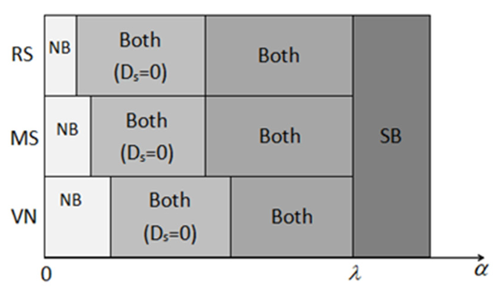
We first compare the critical thresholds for α derived from different power structures with each other to reveal how power structure affects the product strategy of the retailer. To be more intuitive, we present the product strategies under different power structures in Figure 2.
Proposition 1.
For given λ , we can obtain:
(i)
α _ R S < α _ M S < α _ V N ;
(ii)
α ˜ R S = α ˜ M S < α ˜ V N ;
(iii)
α ¯ R S = α ¯ M S = α ¯ V N ;
(iv)
( α α _ G ) λ > 0 , ( α α _ G ) c s < 0 , ( α α _ G ) c n > 0
Proposition 1 implies three main outcomes. First, the power structure does have the impact on the retailer’s introduction strategy of a green store brand in some cases while not in the other cases. More specifically, if the ratio of potential margins is too low or too high, the retailer will decide either not to sell or to sell the green store brand no matter what power structure it is. In the other cases, while α is medium (i.e., α _ R S < α < α _ V N ), the retailer does have reversal strategies under a different power structure.
Secondly, power structures also have impact on the critical threshold values with respect to different product strategies if α < λ and have no effect if α λ . In the latter case, the green store brand is good enough to attract all the consumers, and the retailer will abandon the national brand regardless of supply chain power structure. In the former case, the retailer has the highest threshold to sell both brands and the highest threshold for both brands to have sales under the VN power structure. The mechanism behind this is that the retailer needs to more focus on the balance between both brands under the non-dominated power structure. In addition, it is of interest to note that the retailer is most likely to conduct the both-brands product strategy under the RS power structure. This is because, compared to the MS or VN power structure, the retailer has the absolute priority on pricing under the RS power structure, which assists her in strategic pricing for both brands and benefits from the introduction even if the α is relatively low.
Finally, the higher the consumer green preference and the smaller the unit production cost of the green store brand or the larger the unit production cost of the national brand, the more likely it is for the retailer to introduce the green store brand. That is to say, the category with high consumer green preference and low potential margin of the national brand product enhances the probability for the retailer to cause a profit increase by introducing a green store brand.

5.2. Impacts of Power Structure and Green Store Brand on the Supply Chain Performance

According to the conclusions in Section 5.1, if the α is sufficiently high ( α λ ), the retailer will always sell the green store brand only, and the national brand will exit the market no matter what the power structure it is. As a result, it is intuitive to conclude that the power structure has no effect on the retailer’s pricing decision, and the entry of the green store brand totally changes the supply chain from the manufacturer–retailer with the national brand to only retailer with the green store brand in this case. In another extreme case where the α is sufficiently low ( α α _ R S ), the green store brand will not be introduced, and more power means more preemptive pricing and more profit for the supply chain member, which is consistent with the conclusions in the previous literature (e.g., Choi and Fredj et al., 2013; Ma et al., 2018). Therefore, we next focus our comparisons on the case where the unit production cost of the green store brand is not too low or too high ( α _ R S < α < λ ). By comparing the equilibrium prices, demands, and profits of three supply chain power structures, we can obtain the impacts of power structure on equilibrium results. Furthermore, under each supply chain power structure, we compare the equilibrium results with and without the green store brand to study the impacts of the green store brand on supply chain performance. Let Δ denote the discrepancy in equilibrium resulting from the entry of the green store brand. For example, Δ w R S represents the difference between wholesale prices with and without the green store brand under RS power structure, and Δ w R S = w R S w 0 R S . To identify the difference between equilibrium results under different power structures, various numerical examples are given. Let λ = 4 3 , c n = 1 2 , and c s ( 2 3 , 48 + 29 6 12 ( 3 + 2 6 ) ) ; the interval of c s is derived from the inequality α _ R S < α < λ , which case we focus on. Similarly, let λ = 4 3 , c s = 6 5 , and c n ( 7 2 6 15 , 9 10 ) ; c s = 6 5 , c n = 1 2 , and λ ( 1.2769 , 12 5 ) . These numerical examples also illustrate the effects of parameters on the equilibrium results. Finally, we can obtain the following propositions.
Proposition 2.
(i)
The equilibrium wholesale prices under different power structures are compared as follows:
w 0 M S > w 0 V N > w 0 R S , w M S w V N > w R S ;
(ii)
The difference values in wholesale price under different power structures are compared as follows:
{ Δ w R S < Δ w M S Δ w V N 0       if   2 λ 4 ( 2 λ + 1 ) < α 4 λ 1 4 ( 2 λ 1 ) < α < λ Δ w M S < Δ w R S < Δ w V N 0       if   4 λ 1 4 ( 2 λ 1 ) < α < max ( 16 λ 5 12 ( 2 λ 1 ) , 8 λ 3 ( 4 λ 1 ) ) Δ w M S < Δ w V N < Δ w R S < 0       if   max ( 16 λ 5 12 ( 2 λ 1 ) , 8 λ 3 ( 4 λ 1 ) ) .
Proposition 2 implies that the manufacturer can always charge a higher wholesale price if he has more power regardless of whether the retailer introduces the green store brand. On the other hand, the manufacturer has to decrease the wholesale price facing the entry of green store brand. However, the degree that the wholesale price declines varies from power structures and depends on the values of α and λ . By comparing the three difference values in wholesale price with each other, we can obtain that the wholesale price always declines more under the MS power structure than VN power structure, while it may be more or less under the RS power structure compared to that under the MS/VN power structure. The main implication of this result is that the manufacturer can receive a bigger share of the national brand profit when he has more power in the channel, so he prefers to reduce the wholesale price more to try to keep the consumers from switching to the green store brand.
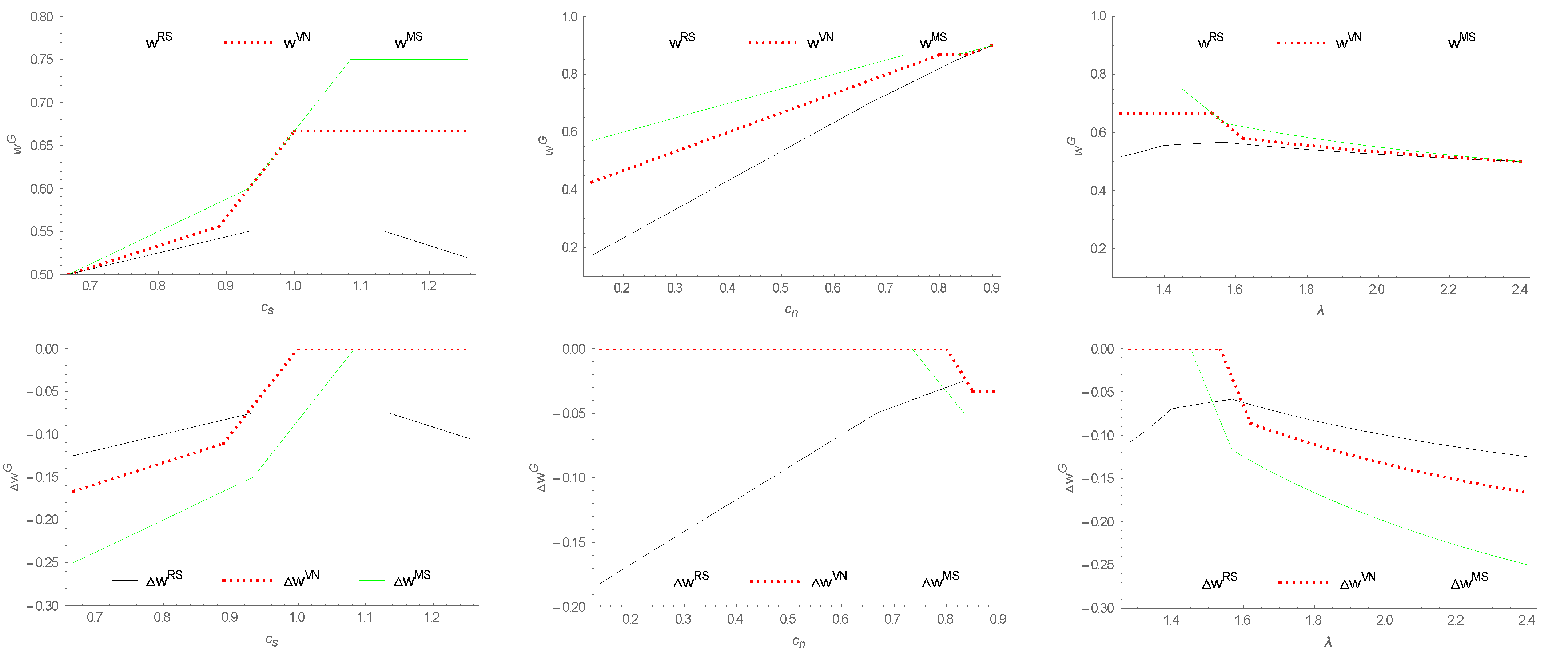
As shown in Figure 3, in most cases, the wholesale price under the MS/VN power structure is increasing in c s an c n and decreasing in λ . It is intuitive that the manufacturer will charge a higher wholesale price if the unit production cost of his own product becomes larger or if the potential margin of the competitor’s product becomes smaller, which implies the stronger advantage in price for the manufacturer’s national brand. However, when power structure is RS, and the α is relatively low, the retailer will introduce the green store brand as a threatening tool, meanwhile utilizing her priority in pricing decision to extract extra profit from the national brand, which results in the fact that the manufacturer has to further cut down the wholesale price of the national brand.
Proposition 3.
(i)
The equilibrium retail margins of the national brand under different power structures are compared as follows:
m 0 M S < m 0 V N < m 0 R S ,   m M S m V N < m R S ;
(ii)
The equilibrium retail prices of green store brand (if introduced) under different power structures are compared as follows:
{ p s R S < p s M S = p s V N = λ + c s 2       if   2 λ 4 ( 2 λ + 1 ) < α < max ( 2 3 , λ 2 λ 1 ) p s R S = p s M S = p s V N = λ + c s 2       if   max ( 2 3 , λ 2 λ 1 ) α < λ ;
(iii)
The difference values in retail margins of national brand under different power structures are compared as follows:
{ Δ m R S > Δ m M S = Δ m V N = 0       if   2 λ 4 ( 2 λ + 1 ) < α λ 2 ( 2 λ 1 ) Δ m M S Δ m V N Δ m R S = 0       if   λ 2 ( 2 λ 1 ) < α < λ .
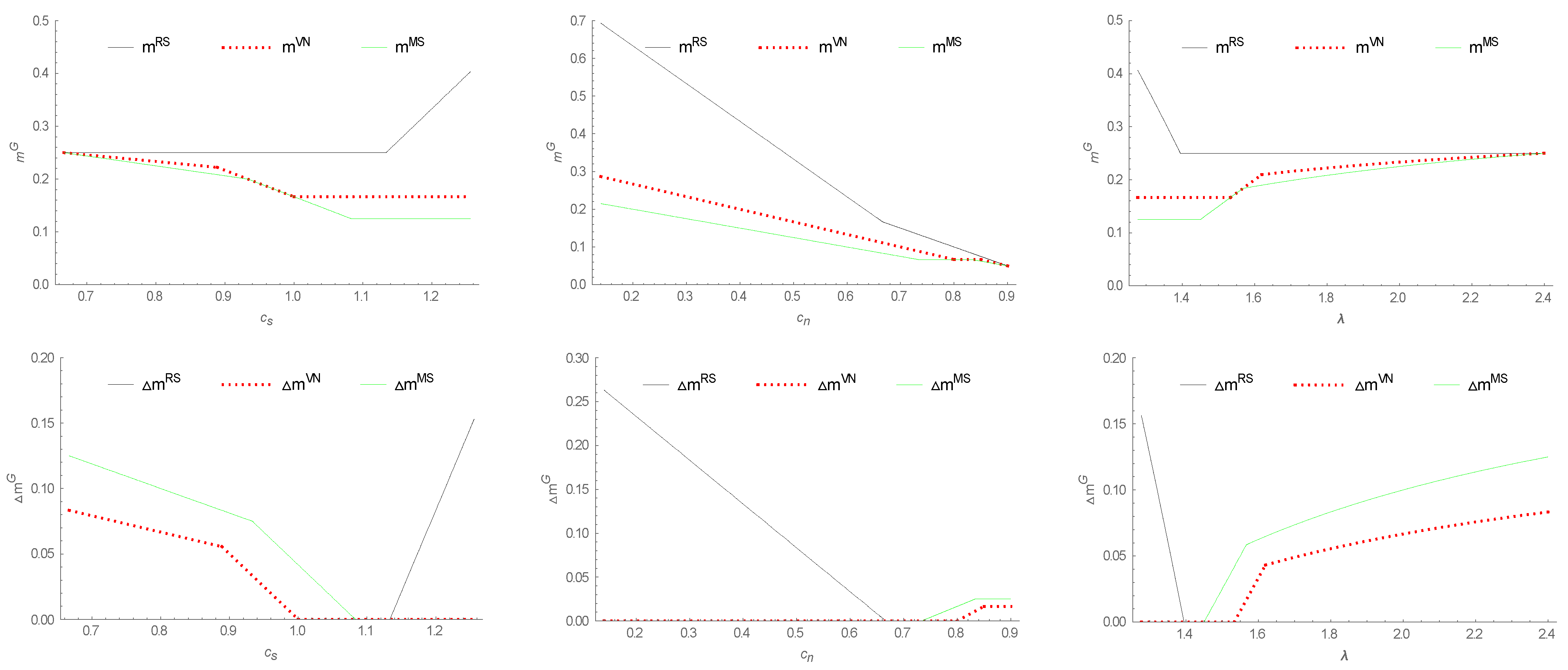
It is not surprising that the retailer can charge a larger retail margin of the national brand for her more power in the supply chain, i.e., the lowest under the MS power structure and highest under the RS power structure, as shown in the upper three pictures of Figure 4. However, it is not the same case with respect to the green store brand. Figure 5 illustrates that the retailer adopts the same pricing strategy for her store brand under different power structures excluding the case in which the power structure is RS, and the α is relatively low. In the latter case, the retailer will set a lower retail price for the green store brand compared to the MS/VN power structure. As a result, according to the equilibrium prices of w G , m G , and p s G under different power structures, we found an unexpected outcome from the retailer’s advantage in decision sequence and the disadvantage in unit production cost of her store brand. That is, the dominant retailer will adopt the price-cutting strategy for the green store brand to compel the manufacturer to further reduce the wholesale price, and then, the retailer can achieve more margin on the national brand. However, this price-cutting strategy is not useful when the retailer does not have the priority on pricing, which leads to the price strategy for the green store brand (if it is introduced) in these cases remaining unchanged with the decrease of α .
By comparing the equilibrium retail margins on the national brand before and after the entry of the green store brand, we can obtain that the retailer will always set a higher margin on the national brand after the entry of the green store brand, as shown in the three pictures at the bottom of Figure 4. The motivation behind this is not only to cause more sharing of the sale of the national brand but also to make room for the sale of the green store brand.
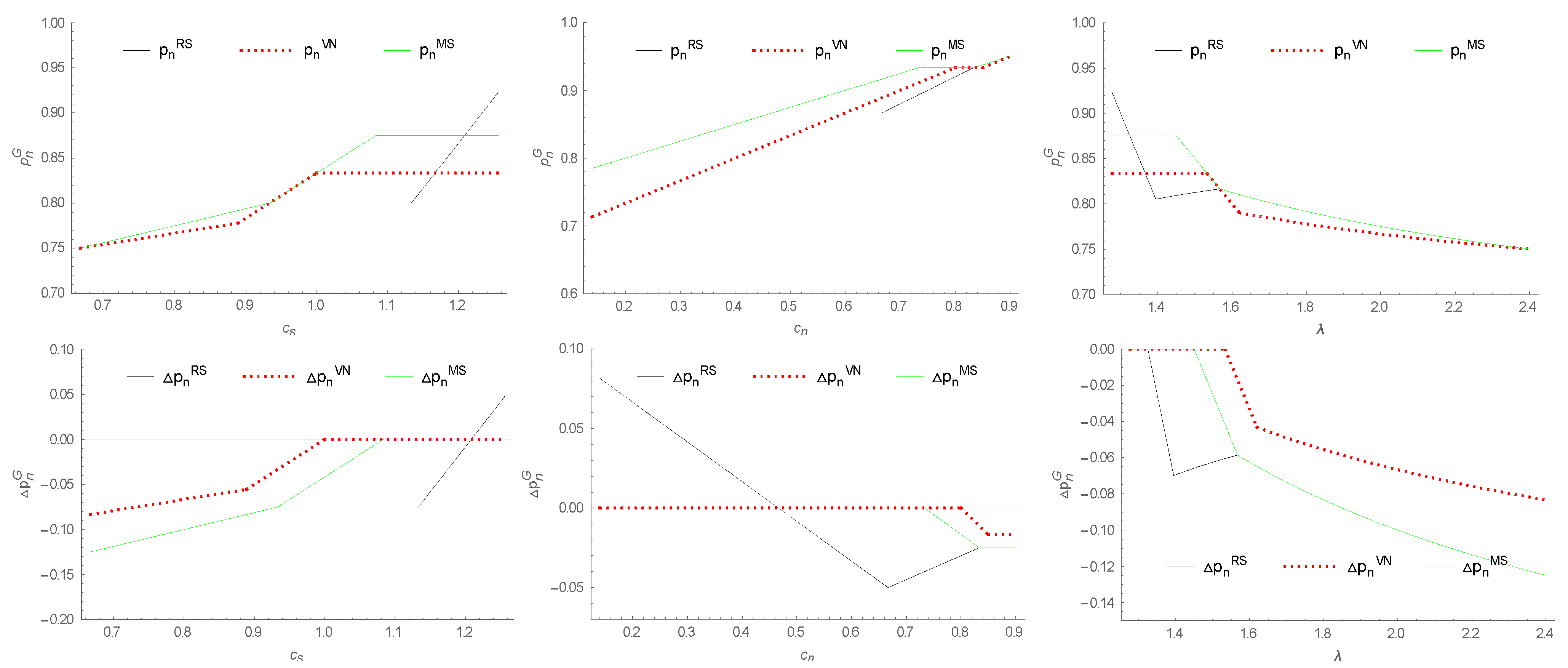
Moreover, Figure 4 illustrates that the impacts of three parameters on the retail margin of national brand vary between different intervals and different power structures. In sum, only when the power structure is RS, and the α is relatively low does the retail margin m R S increase in c s and decrease in λ ; furthermore, the retail margin m R S is non-inclined with increasing c n and c s and non-declined with increasing λ . Figure 5 illustrates that when the retailer does not adopt the price-cutting strategy for the green store brand, the retail price only depends on the value of λ and c s and is increasing in λ and c s . However, when the retailer adopts the price-cutting strategy, she also should take the unit production cost c n into consideration, and all three parameters may increase the retail price p s R S in some cases but have no impact on it in the other cases.
Proposition 4.
(i)
The equilibrium retail prices of national brand under different power structures are compared as follows:
p n 0 M S = p n 0 R S > p n 0 V N ,  
  • and
{ p n R S p n M S > p n V N           if   2 λ 4 ( 2 λ + 1 ) < α 1 4 p n M S > p n R S p n V N           if 1 4 < α 1 3 p n M S p n V N p n R S           if   1 3 < α < 1 2 λ 1 p n M S = p n R S > p n V N           if   1 2 λ 1 α < λ ;
(ii)
The difference values in retail margins of national brand under different power structures are compared as follows:
{ Δ p n R S > Δ p n M S = Δ p n V N = 0           if   2 λ 4 ( 2 λ + 1 ) < α 1 4 Δ p n R S Δ p n M S Δ p n V N 0           if   1 4 < α < λ .
Before the introduction of the green store brand, the retail price of the national brand is lowest under VN power structure, and this remains after the entry of the green store brand except in the situation where the retailer is a leader, and the α is medium-high, as shown in the upper three pictures in Figure 6. This indicates that the non-dominated supply chain power structure alleviates the double-marginalization problem for the national brand, which is consistent with Choi (1991) [26], Chung and Lee (2017) [28], and Luo et al. (2017) [17]. For the special result that p n M S p n V N p n R S , it can be explained by the comprehensive effect of power structure and green store brand; that is, the mitigation effect of the latter on double-marginalization problem (implied by Proposition 4(ii)) is greater than the former.
Proposition 4 (ii) states that the green store brand also can alleviate the double-mitigation effect of the national brand in most cases, which is in accordance with the conclusions in Sayman and Raju (2004) [10], Choi, (2006) [21], Chen et al. (2011) [15], and Xiang Fang et al. (2013) [16]. However, different from the previous literature, we find the unexpected result that the green store brand may deteriorate the double-mitigation effect of national brand when the power structure is RS, and the α is relatively low, as shown in the lower three pictures in Figure 6. The mechanisms for the two opposite effects on the double-mitigation effect can be derived by the conclusions in the above propositions relative to the wholesale price and retail margin of the national brand. That is, the reduction in double-mitigation effect comes from a lower wholesale price, and the deterioration comes from a higher retail margin.
Proposition 5.
(i)
The equilibrium profits of the retailer under different power structures are compared as follows:
π R 0 M S < π R 0 V N < π R 0 R S , π R M S π R V N < π R R S ,  
  • and
{ Δ π R R S Δ π R M S Δ π R V N 0         if 2 λ 4 ( 2 λ + 1 ) < α 1 + 2 λ 4 2 λ 1 Δ π R M S > Δ π R R S > Δ π R V N 0         if   λ < 1 14 ( 7 + 3 7 ) a n d 1 + 2 λ 4 2 λ 1 < α < λ ( λ 1 ) ( 16 λ 2 14 λ 1 ) 3 λ 3 ( 2 λ 2 4 λ + 1 ) or   λ 1 14 ( 7 + 3 7 ) a n d 1 + 2 λ 4 2 λ 1 < α < 1 + 16 λ 3 2 ( 2 λ 1 ) Δ π R M S > Δ π R V N Δ π R R S > 0         if   λ < 1 14 ( 7 + 3 7 ) a n d λ ( λ 1 ) ( 16 λ 2 14 λ 1 ) 3 λ 3 ( 2 λ 2 4 λ + 1 ) α < λ or λ 1 14 ( 7 + 3 7 ) a n d 1 + 16 λ 3 2 ( 2 λ 1 ) α < λ ;
(ii)
The equilibrium profits of the manufacturer under different power structures are compared as follows:
π M 0 M S > π M 0 V N > π M 0 R S , π M M S π M V N > π M R S ,  
  • and
{ Δ π M R S < Δ π M M S Δ π M V N 0         if   2 λ 4 ( 2 λ + 1 ) < α 2 + 2 4 ( 2 λ 1 ) Δ π M M S < Δ π M R S < Δ π M V N < 0         if   2 + 2 4 ( 2 λ 1 ) < α < 1 2 + 2 ( 8 λ 2 8 λ + 11 ) 12 ( 2 λ 1 ) Δ π M M S < Δ π M V N Δ π M R S < 0         if   1 2 + 2 ( 8 λ 2 8 λ + 11 ) 12 ( 2 λ 1 ) α < λ .
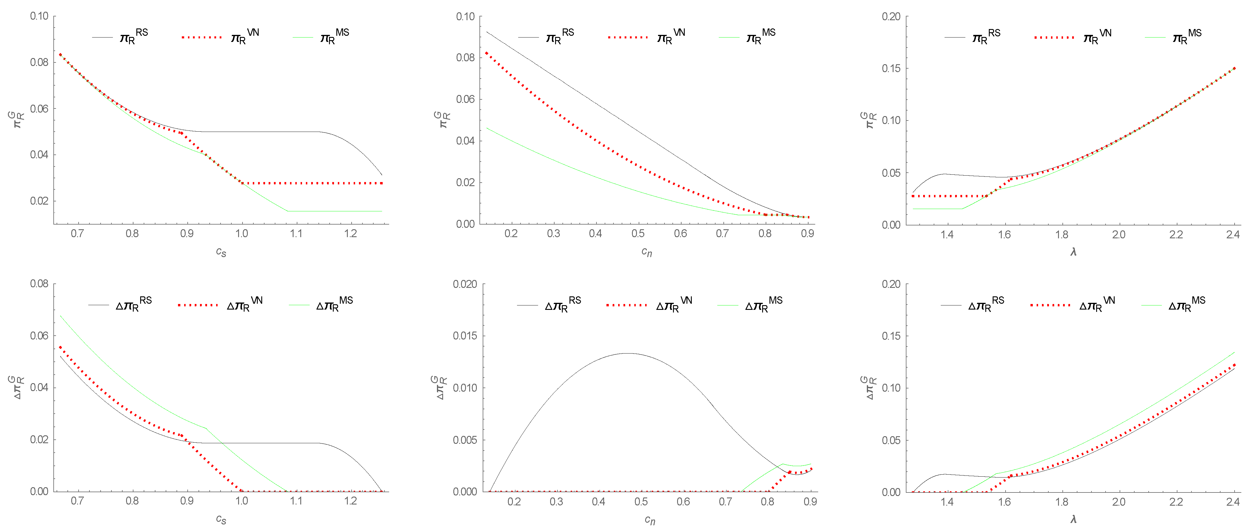
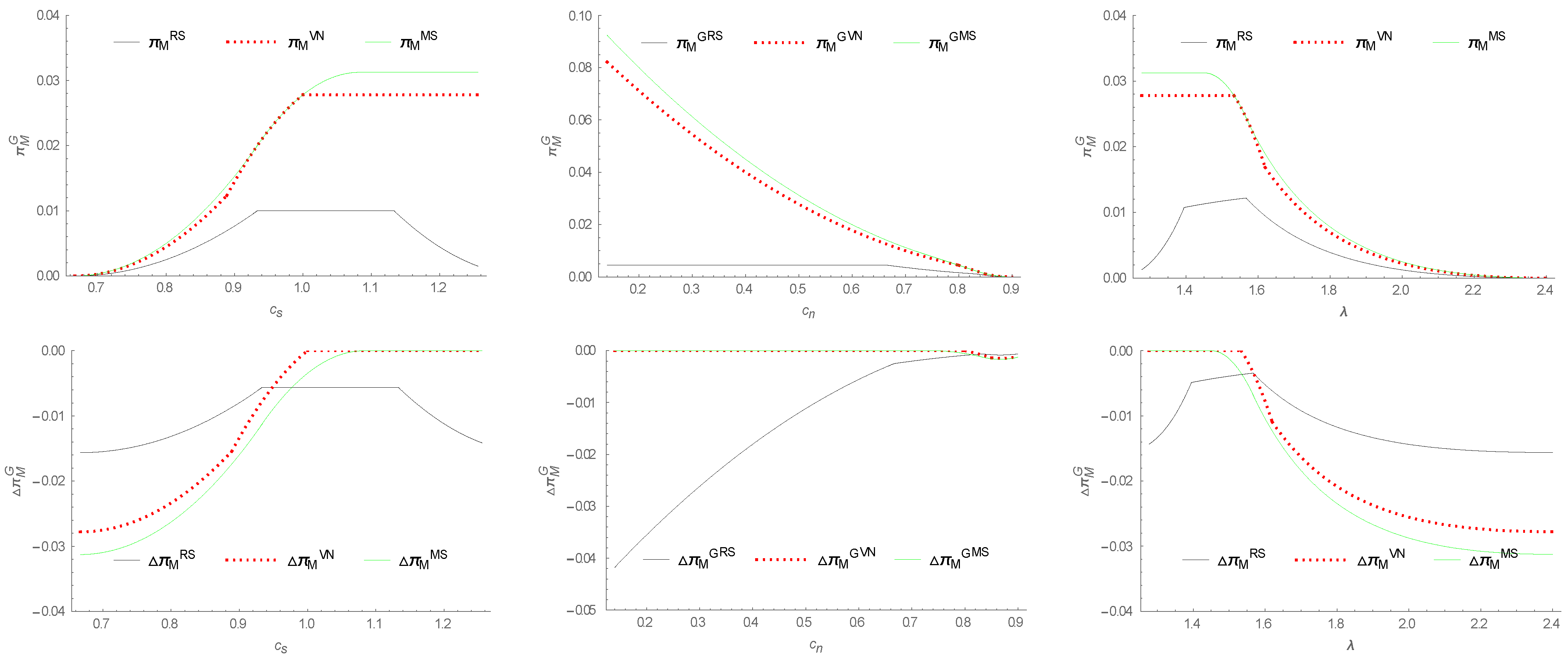
By comparing the profits of retailer or manufacturer derives from three power structures, respectively, before and after the introduction of the green store brand, we can obtain that, regardless of the green store brand introduction, the supply chain member always gains more profit with bigger power, as shown in the upper pictures in Figure 7 and Figure 8. Figure 7 and Figure 8 also illustrate the impacts of three parameters on the profits of the retailer and manufacturer. When the green store brand is introduced as a profitable product, the profit of retailer increases in λ and decreases in c s and c n , while the profit of the manufacturer increases in c s and decreases in λ and c n . This finding may remain when the green store brand is introduced as a threatening tool except for the case where the power structure is RS, and the α is relatively low. In the latter case, we were surprised to find that the manufacturer benefits from the improvement of the green store brand’s potential margin, and this may result from the declining threat of the green store brand with higher potential margin. Further, the manufacturer’s profit is unchanged in c n within a certain interval, which means the manufacturer may fail to improve his profit by attempting to lower the unit production cost. It is also interesting to find that, in this case, the retailer’s profit decreases in λ within a certain interval and is unchanged in c s within a certain interval, which means the retailer does not always benefit from the higher consumers’ green preference and does not always suffer from the incline of unit production cost.
On the other hand, regardless of power structure, once the conditions for the introduction of the green store brand are satisfied, the retailer will benefit from the entry of the green store brand, while the manufacturer will suffer from it. However, the degree of profit increase or decrease varies between different power structures. More specifically, while the ratio is sufficiently high, meaning the green store brand is competitive and has positive demand, then the power structure plays the “Curse of God” for both supply chain members. However, with the decreasing of ratio, the retailer will introduce the green store brand as a threatening tool instead of a profitable product, and the “Curse of God” may disappear. As a result, compared to the other two power structures, the retailer under the RS power structure may gain more profits due to the entry of the green store brand, and simultaneously, the manufacturer may lose more in this situation. This gives an interesting insight into the problem of the green store brand’s introduction for the retailer. That is, for the category in which the potential margin of national brand is too high for green store brand to achieve the relatively competitive potential margin, the retailer should position the green store brand against the weak manufacturer. On the contrary, the strong manufacturer will be against for the category in which the green store brand has enough advantage on the potential margin.

6. Conclusions

6.1. Theoretical Implications

With the rapid development of the retail industry, both store brands and supply chain power structure have undergone the key changes. For the store brand, it is not just an inferior substitute for national brands anymore but a product with its own special value. The green store brand, one kind of burgeoning store brand, has a very different market positioning compared to the traditional store brand. While the traditional one targets the price-oriented consumers, the green store brand targets value-oriented consumers. In other words, the product attributes between the two kinds of store brand are totally different. However, previous studies have mainly focused on the traditional store brand, and the issues of when and where to introduce a green store brand remain unclear. In this paper, we investigate the conditions for a retailer to introduce a green store brand and the impacts of the introduction of a green store brand on the supply chain equilibrium. On the other hand, for the supply chain power structure, there exists different power structures according to the ability of the retailer to negotiate with the manufacturer. The previous literature with respect to the power structure and store brand mainly focused on the coordination of the supply chain with a store brand. Our work, different from these literatures, studies how the power structure affects the introduction of store brand.
In sum, the main contributions of this paper are in recognizing the conditions associate with introducing a green store brand and investigating the impacts of power structure on the introduction of a green store brand as well as the impacts of a green store brand on supply chain performance under different power structures. Our main findings are as follows:
Firstly, the retailer has the lowest threshold to introduce the green store brand when she is a leader in the supply chain and the highest threshold in the non-dominant supply chain. Further, under each power structure, the possibility of introduction becomes larger with the increasing consumer green preference, the decreasing unit production cost of the green store brand, and the increasing unit production cost of the national brand.
Secondly, if the green store brand is introduced, it may be used as a profitable product or a just threatening tool, which depends on the potential margin ratio of the green store brand to the national brand. If this critical ratio is lower than the corresponding threshold ( α ˜ G ), the green store brand will be introduced but have no sales, meaning that it could be an effective tool to force the manufacturer to make concessions in wholesale price. Otherwise, the green store brand will have positive demand and even may kick the national brand out of the market. Furthermore, the green store brand is most likely introduced as a profitable product instead of a threatening tool under the VN power structure, while it has the same functional position under the MS and RS power structures.
Thirdly, regardless of power structure, as long as the critical ratio is higher than the certain lower threshold, the retailer will always benefit, while the manufacturer will always suffer from the introduction of green store brand, which is different from the conclusions in Ru et al. (2015) [12] and Ma et al. (2018) [31]. They stated that the manufacturer may benefit from the store brand. Furthermore, if the green store brand is introduced as a profitable product, the supply chain member will benefit or suffer most under the MS power structure and least under RS power structure. However, it is not necessary when the green store brand is used as a threatening tool. Moreover, even though the increase or decrease of profits of supply chain members varies under different power structures, the supply chain members still can gain more profits with stronger power.
Finally, we found the conclusion in previous literature that the non-dominant supply chain power structure can alleviate the double-marginalization problem for the national brand and still satisfy the supply chain with a green store brand. Besides this, we also find that the entry of green store brand could alleviate the double-marginalization problem in most cases, which is consistent with Sayman and Raju (2004) [10], Ru et al. (2015) [12], Mills (1995) [13], and Chen et al. (2011) [15]. However, what is different from these previous studies is our finding that the green store brand may aggravate the double-mitigation effect of the national brand if the power structure is RS, and the α is relatively low.

6.2. Managerial Implications

Our results offer some meaningful managerial insights to the supply chain members as well as the government. Firstly, for the retailer, the optimal introduction and product strategies depend on the power structures and the relevant parameters, which means that for a given green product the retailer can offer, she may make different choices under different relationships between her and the manufacturer. In addition, according to the potential margin ratio, she can introduce the green store brand under different roles, i.e., either as just a threatening tool or as a profitable product. In turn, the retailer should choose the best pricing strategies for the green store brand on the basis of its role and power structures. More specifically, when the power structure is RS, and the potential margin ratio is low but still higher than the introduction threshold, the retailer should take a pricing-cutting strategy for her green store brand. Furthermore, the retailer can always benefit from the stronger negotiation strength, and she should try her best to improve consumer loyalty.
Secondly, for the manufacturer, enhancing the negotiation strength and cutting down the unit production cost of national brand are the main two approaches to improve his profit. In the supply chain with a green store brand, the former one is always useful, while the latter one is ineffective if the manufacturer is the follower, and the green store brand is positioned as a threatening tool. Therefore, the manufacturer should take a careful consideration about whether to take actions to cut the cost. However, he could always make measures such as advertising to enhance the negotiation strength and realize the profit increase.
Finally, for the government, he could take some measures to encourage the retailer to introduce the green store brand. For example, the government can conduct green propaganda to enhance the consumers’ green preference; he also can instate a tax remission or offer a technical guidance to lower the unit production cost of the green store brand. However, what is most important is that the government should ensure that the green store brand has real sales to make potential policies or actions meaningful in the aspect of environmental protection (by promoting the green product) and in the aspect of supply chain management (by eliminating the possible aggravation effect brought by the green store brand on the double-marginalization problem for national brand).

6.3. Limitation and Future Research

There are some limitations of our research that can be extended in the following ways. First, we assume all consumers have the same green product preference; however, it may not always be the truth. In fact, the difference in personal characteristics, such as age, education, and experience, may lead to different green preferences. It will be interesting to take this heterogeneity into consideration. Furthermore, we only consider the supply chain of a single manufacturer and a single retailer. However, a supply chain with multiple manufacturers and multiple retailers is more common in reality. Therefore, one can extend our work by considering multiple retailers who are all interested in introducing their own store brands. Additionally, to allow the manufacturer to sell the national brand through his own direct channel and study the interaction under the dual-channel supply chain will be another direction to extent our study. Finally, it is important to validate our results through an empirical study with real data.

Author Contributions

Conceptualization, J.Z. and J.H.; methodology, J.Z.; software, J.Z.; validation, J.Z. and J.H.; formal analysis, J.Z.; investigation, J.Z.; resources, J.H.; data curation, J.Z.; writing—original draft preparation, J.Z.; writing—review and editing, J.Z. and J.H.; visualization, J.Z.; supervision, J.H.; project administration, J.H.; funding acquisition, J.H. All authors have read and agreed to the published version of the manuscript.

Funding

This research was supported by National Natural Science Foundation of China (Grant No. 71532015).

Conflicts of Interest

The author declares no conflict of interest.

Appendix A

Proof of Lemma 1.
In the MS game, the manufacturer first sets the wholesale price w M S , and then the retailer, given the value of w M S , sets m M S and p s M S to maximize her profit. First, we derive the optimal m M S and p s M S for either of the following three cases. □
(1)
m M S p s M S λ + 1 w M S
In this case, only national brand has sales. Thus, the optimal prices are determined by solving the following problem:
max π R 1 M S ( m M S ) = m M S ( 1 m M S w M S ) s . t .   m M S p s M S λ + 1 w M S
According to 2 π R 1 M S m M S 2 = 2 < 0 , we can obtain that π R 1 M S ( m M S ) is a concave function. By letting π R 1 M S m M S = 0 , we can obtain the optimal retail margin m 1 M S * = 1 w M S 2 , and the retail price of the green store brand p s 1 M S * should satisfy the constraint p s 1 M S * max { c s , λ 1 w M S * 2 } . Replacing it into the retailer’s profit function yields π R 1 M S * = ( 1 w M S ) 2 4 .
(2)
p s M S λ + 1 w M S < m M S < p s M S λ w M S
In this case, both brands have sales. Hence, the optimal prices are determined by solving the following problem:
max π R 2 M S ( m M S , p s M S ) = m M S ( p s M S m M S w M S λ 1 m M S w M S ) + ( p s M S c s ) ( 1 p s M S m M S w M S λ 1 ) s . t .   p s M S λ + 1 w M S < m M S < p s M S λ w M S
Taking the partial derivative of π R 2 M S with respect to m M S and p s M S , we can obtain the Hessian matrix:
H 1 = [ 2 π R M S m M S 2 2 π R M S m M S p s M S 2 π R M S p s M S m M S 2 π R M S p s M S 2 ] = [ 2 λ λ 1 2 λ 1 2 λ 1 2 λ 1 ]
where the first-order principal minor is 2 λ λ 1 < 0 , and the second-order principal minor is 4 λ ( λ 1 ) 2 4 ( λ 1 ) 2 = 4 λ 1 > 0 , the H1 is thus a negative definite matrix. By letting π R 2 M S m M S = 0 and π R 2 M S p s M S = 0 , we can obtain the optimal retail margin m 2 M S * = 1 w M S 2 and p s 2 M S * = λ + c s 2 . The constraint should be satisfied, and simplifying p s 2 M S * λ + 1 w M S < m 2 M S * < p s 2 M S * λ w M S yields 1 + c s λ < w M S < c s λ . In addition, replacing m 2 M S * = 1 w M S 2 and p s 2 M S * = λ + c s 2 into the retailer’s profit function yields π R 2 M S * = ( 1 w M S ) 2 4 + ( λ c s 1 + w M S ) 2 4 ( λ 1 ) .
(3)
m M S p s M S λ w M S
In this case, only green store brand has sales. Therefore, the optimal prices are determined by solving the following problem:
max π R 3 M S ( p s M S ) = ( p s M S c s ) ( 1 p s M S λ ) s . t .   m M S p s M S λ w M S
According to 2 π R 3 M S p s M S 2 = 2 λ < 0 , we can obtain that π R 3 M S ( p s M S ) is a concave function. By letting π R 3 M S p s M S = 0 , we can obtain the optimal retail price of the green store brand p s 3 M S * = λ + c s 2 λ , and the retail margin m 3 M S should satisfy the constraint condition of m 3 M S * λ + c s 2 λ w M S . Replacing it into the retailer’s profit function yields π R 3 M S * = ( λ c s ) 2 4 λ .
Next, we compared the three optimal profits of retailer derived from the above cases. Note that if 1 + c s λ < w M S < c s λ , then π R 2 M S * w M S = λ w M S c s 2 ( λ 1 ) . It is easy to obtain that π R 2 M S * w M S = λ w M S c s 2 ( λ 1 ) π R 2 M S * w M S | ( w M S = c s λ ) = 0 . Therefore, π R 2 M S * is decreasing in w M S when 1 + c s λ < w M S < c s λ . Based on this, we have the following comparisons:
For w M S 1 + c s λ , π R 2 M S * < π R 2 M S * ( w M S = 1 + c s λ ) = ( 1 w M S ) 2 4 = π R 1 M S * , and π R 1 M S * π R 3 M S * = ( 1 w M S ) 2 4 ( λ c s ) 2 4 λ ( λ c s ) 2 4 ( λ c s ) 2 4 λ > 0 . Therefore, if w M S min { 0 , 1 + c s λ } , the optimal prices of both brands are m M S * = ( 1 w M S ) 2 4 and p s M S * = N / A .
For 1 + c s λ < w M S < c s λ , then π R 2 M S * > π R 2 M S * ( w M S = c s λ ) = ( λ c s ) 2 4 λ = π R 3 M S * , and π R 2 M S * π R 1 M S * = ( λ c s 1 + w M S ) 2 4 ( λ 1 ) > 0 . Therefore, if { 0 , 1 + c s λ } < w M S < c s λ , the optimal prices of both brands are m M S * = 1 w M S 2 and p s M S * = λ + c s 2 .
For w M S c s λ , then π R 2 M S * < π R 2 M S * ( w M S = c s λ ) = ( λ c s ) 2 4 λ = π R 3 M S * , and π R 3 M S * π R 1 M S * > π R 3 M S * π R 1 M S * ( w M S = c s λ ) = ( λ 1 ) ( λ c s ) 2 4 λ 2 > 0 . Therefore, if w M S c s λ , the optimal prices of both brands are m M S * = N / A and p s M S * = λ + c s 2 .
In summary, for a given w M S , the optimal retail margins of both brands are as follows:
( m M S * , p s M S * ) = { ( 1 w M S 2 , N / A ) if   w M S 1 + c s λ ( 1 w M S 2 , λ + c s 2 )   if   1 + c s λ < w M S < c s λ ( N / A , λ + c s 2 )       if   w M S c s λ .
Proof of Lemma 2.
The manufacturer’s optimal wholesale price w M S * is derived using a two-step analysis: First, we obtained the optimal w M S for each of the three cases. Then, by comparing the three optimal profits of manufacturer derived from the above cases, we can obtain the overall optimal wholesale price w M S * . □
(1)
w M S 1 + c s λ
In this case, the optimal w 1 M S is determined by solving the following problem:
max π M 1 M S ( w M S ) = ( w M S c n ) ( 1 w M S ) 2 s . t .   w M S 1 + λ c s
According to π M 1 M S w M S = 1 < 0 and letting π M 1 M S w M S = 0 , we can obtain the optimal wholesale price w 1 M S * = 1 + c n 2 , and simplifying 1 + c n 2 1 + c s λ yields α < 1 2 . That is to say, if α 1 2 , the π M 1 M S is increasing in w M S when w M S 1 + c s λ . Furthermore, note that the w M S > c n should be satisfied for the positive profit of manufacturer, and simplifying c n < 1 + c s λ yields α < 1 . Therefore, if 1 2 α < 1 , then w 1 M S * = 1 + c s λ , and otherwise, w 1 M S * = N / A .
As a result, the manufacturer’s optimal wholesale price w 1 M S in this case can be presented as follows:
w 1 M S * = { 1 + c n 2   if   α 1 2 1 + c s λ   if   1 2 < α < 1 N / A   if   α 1
(2)
1 + c s λ < w M S < c s λ
In this case, the optimal w 2 M S is determined by solving the following problem:
max π M 2 M S ( w M S ) = ( w M S c n ) ( c s λ w M S ) 2 λ 1 s . t .   1 + c s λ < w M S < c s λ
According to 2 π M 2 M S w M S 2 = 2 λ 2 λ 1 < 0 and letting π M 2 M S w M S = 0 , we can obtain the optimal wholesale price w 2 M S * = c s + λ c n 2 λ , and simplifying 1 + c s λ < c s + λ c n 2 λ < c s λ yields λ 2 λ 1 < α < λ . Similar to the above case, the manufacturer’s optimal wholesale price w 2 M S * in this case can be presented as follows:
w 2 M S * = { 1 + c s λ + ε     if   α λ 2 λ 1 c s + λ c n 2 λ     if   λ 2 λ 1 < α < λ N / A         if   α λ
(3)
w M S c s λ
In this case, the national brand will never have sales and the manufacturer’s profit always equals to zero.
Next, by comparing π M 1 M S * ( w 1 M S * ) , π M 2 M S * ( w 2 M S * ) , and π M 3 M S * ( = 0 ) with each other, we can obtain the overall optimal w M S * . Note that 1 2 < λ 2 λ 1 < 1 < λ , and the manufacturer’s optimal wholesale price can be fully characterized based on which of the intervals α falls into.
For α 1 2 , π M 1 M S * ( 1 c n 2 ) π M 1 M S * ( 1 λ + c s ) > π M 2 M S * ( 1 λ + c s + ε ) > π M 3 M S * = 0 ;
For 1 2 < α λ 2 λ 1 , π M 1 M S * ( 1 λ + c s ) > π M 2 M S * ( 1 λ + c s + ε ) > π M 3 M S * = 0 ;
For λ 2 λ 1 < α < 1 , π M 1 M S * ( 1 λ + c s ) < π M 2 M S * ( c s + λ c n 2 λ ) , and π M 2 M S * ( c s + λ c n 2 λ ) > π M 3 M S * = 0 ;
For 1 α < λ , π M 2 M S * ( c s + λ c n 2 λ ) > π M 1 M S * = π M 3 M S * = 0 ;
For α λ , π M 1 M S * = π M 2 M S * = π M 3 M S * = 0 .
In summary, we can obtain the optimal w M S * as follows:
w M S * = { 1 + c n 2   if   α 1 2 1 + c s λ   if   1 2 < α λ 2 λ 1 c s + λ c n 2 λ       if   λ 2 λ 1 < α < λ N / A   if   α λ
Proof of Theorem 1.
If the retailer does not introduce the green store brand, then we have the equilibrium results, which are shown in Section 4.1.1. Denote the corresponding profit of retailer by π R 0 M S and π R 0 M S = ( 1 c n ) 2 16 . On the contrary, if the retailer introduces the green store brand, then her optimal profit for a given pair of α and λ is presented as follows:
π R M S * = { ( 1 c n ) 2 16   if   α 1 2 ( λ c s ) 2 4   if   1 2 < α λ 2 λ 1 ( c s λ c n ) 2 + 4 ( λ 1 ) ( λ c s ) 2 16 λ ( λ 1 )   if   λ 2 λ 1 < α < λ ( λ c s ) 2 4 λ   if   α λ .
Obviously, (1) if α 1 2 , then π R M S * = π R 0 M S * . (2) If 1 2 < α λ 2 λ 1 , then π R M S * π R 0 M S * = ( λ c s ) 2 4 ( 1 c n ) 2 16 = ( 1 c n ) 2 ( 2 α + 1 ) ( 2 α 1 ) 16 > 0 . (3) If λ 2 λ 1 < α < λ , then π R M S * π R 0 M S = ( c s λ c n ) 2 + 4 ( λ 1 ) ( λ c s ) 2 16 λ ( λ 1 ) ( 1 c n ) 2 16 = ( 1 c n ) 2 [ ( λ α ) 2 + 4 ( λ 1 ) α 2 λ ( λ 1 ) ] 16 λ ( λ 1 ) . Let F ( α ) = ( λ α ) 2 + 4 ( λ 1 ) α 2 λ ( λ 1 ) ; we can have F ( α ) = 2 ( λ α ) + 8 ( λ 1 ) α = 2 [ ( 4 λ 3 ) α λ ] and F ( α ) = 2 ( 4 λ 3 ) > 0 . Thus, F ( α ) is increasing in α . As a result, F ( α ) > F ( λ 2 λ 1 ) = λ ( 4 λ 3 2 λ 1 1 ) = 2 λ ( λ 1 ) 2 λ 1 > 0 . Therefore, F ( α ) is increasing in α , and F ( α ) > F ( λ 2 λ 1 ) = λ ( λ 1 ) ( 4 λ 1 ) ( 2 λ 1 ) 2 > 0 , which implies that π R M S * π R 0 M S > 0 . (4) If α λ , then π R M S * π R 0 M S = ( λ c s ) 2 4 λ ( 1 c n ) 2 16 = ( 1 c n ) 2 ( 2 α + λ ) ( 2 α λ ) 16 λ > 0 .
Therefore, we summarize the retailer’s optimal product strategy as follows. The retailer will sell the only national brand if α 1 2 and only the green store brand if α λ ; otherwise, she will sell both brands. More specifically, replacing the optimal prices into the demand functions of both brands while the retailer sells both brands, we find that both brands have sales only when λ 2 λ 1 < α < λ ; otherwise, the demand of the green store brand will be zero.
Proof of Lemma 3.
In the RS game, the retailer first sets the m R S and p s R S to maximize her profit, and then, the manufacturer, given the values of m R S and p s R S , sets wholesale price w R S to maximize his profit. We derive the optimal wholesale price for either of the following three cases. □
(1)
w R S 1 + p s R S λ m R S
In this case, the optimal w 1 R S * is determined by solving the following problem:
max π M 1 R S ( w R S ) = ( w R S c n ) ( 1 w R S m R S ) s . t .   w R S 1 + p s R S λ m R S
According to π M 1 R S w R S = 2 < 0 , we can obtain that π M 1 R S ( w R S ) is a concave function. Letting π M 1 R S w R S = 0 and π M 1 R S w R S = 1 2 w R S m R S + c n , we can obtain the optimal wholesale price w 1 R S * = 1 m R S + c n 2 , and simplifying 1 m R S + c n 2 1 + p s R S λ m R S yields m R S 1 c n 2 ( λ p s R S ) . That is to say, the optimal wholesale price w 1 R S * = 1 m R S + c n 2 if m R S 1 c n 2 ( λ p s R S ) ; otherwise, the π M 1 R S is increasing in w R S when w R S 1 + p s R S λ m R S . Therefore, if m R S > 1 c n 2 ( λ p s R S ) , then the optimal w 1 R S * = 1 + p s R S λ m R S .
(2)
1 + p s R S λ m R S < w R S < p s R S λ m R S
In this case, the optimal w 2 R S * is determined by solving the following problem:
max π M 2 R S ( w R S ) = ( w R S c n ) ( p s R S m R S w R S λ 1 m R S w R S ) s . t .   1 + p s R S λ m R S < w R S < p s R S λ m R S
According to 2 π M 2 R S w R S 2 = 2 λ λ 1 < 0 , we can obtain that π M 2 R S ( w R S ) is a concave function. Letting π M 2 R S w R S = 0 and π M 2 R S w R S = λ ( c n 2 w R S m R S ) + p s R S λ 1 , we can obtain w 2 R S * = λ ( c n m R S ) + p s R S 2 λ , and simplifying 1 + p s R S λ m R S < λ ( c n m R S ) + p s R S 2 λ < p s R S λ m R S yields 2 ( 1 λ + p s R S ) c n p s R S λ < m R S < p s R S λ c n . Similar to the above case, if m R S 2 ( 1 λ + p s R S ) c n p s R S λ or m R S p s R S λ c n , then π M 2 R S is decreasing or increasing in w R S when 1 + p s R S λ m R S < w R S < p s R S λ m R S . As a result, the optimal wholesale price w 2 R S * = 1 + p s R S λ m R S + ε in the former case and w 2 R S * = N / A in the latter case.
(3)
w R S p s R S λ m R S
In this case, the national brand will never have sales, and the manufacturer’s profit always equals to zero.
Next, we compared the three optimal profits of manufacturer derived from the above cases. Note that for any p s R S < λ , we have 1 c n 2 ( λ p s R S ) < 2 ( 1 λ + p s R S ) c n p s R S λ < p s R S λ c n . Hence, we derived the optimal wholesale price w R S * under different regions with respect to m R S and p s R S as follows.
If m R S 1 c n 2 ( λ p s R S ) , then
π M 1 R S * ( w 1 R S * = 1 m R S + c n 2 ) > π M 1 R S ( w 1 R S = 1 + p s R S λ m R S ) > π M 2 R S * ( w 2 R S = 1 + p s R S λ m R S + ε ) > π M 3 R S * ;
If 1 c n 2 ( λ p s R S ) < m R S 2 ( 1 λ + p s R S ) c n p s R S λ , then
π M 1 R S * ( w 1 R S * = 1 + p s R S λ m R S ) > π M 2 R S * ( w 2 R S * = 1 + p s R S λ m R S + ε ) > π M 3 R S * ;
If 2 ( 1 λ + p s R S ) c n p s R S λ < m R S < p s R S λ c n , then
π M 2 R S * ( w 2 R S * = λ ( c n m R S ) + p s R S 2 λ ) > π M 2 R S ( w 2 R S * = 1 + p s R S λ m R S + ε ) > π M 1 R S * ( w 1 R S * = 1 + p s R S λ m R S ) > π M 3 R S * ;
If m R S p s R S λ c n , then for any w R S > c n , there always is m R S + w R S p s R S λ , which implies D n 0 . Hence, π M 1 R S = π M 2 R S = π M 3 R S = 0 .
In summary, we can obtain the optimal w R S * as follows:
w R S * = { 1 m R S + c n 2         if   m R S 1 c n 2 ( λ p s R S ) 1 + p s R S λ m R S   if   1 c n 2 ( λ p s R S ) < m R S 2 ( 1 λ + p s R S ) c n p s R S λ λ ( c n m R S ) + p s R S 2 λ   if   2 ( 1 λ + p s R S ) c n p s R S λ < m R S < p s R S λ c n N / A   if   m R S p s R S λ c n
Proof of Lemma 4.
The retailer, anticipating the manufacturer’s optimal wholesale price w R S * , sets m R S and p s R S to maximize her profit. We derive the optimal m R S and p s R S for either of the following four cases. □
(1)
m R S 1 c n 2 ( λ p s R S )
In this case, only national brand has sales. Thus, the optimal prices are determined by solving the following problem:
max π R 1 R S ( m R S ) = m R S ( 1 m R S c n ) 2 s . t .   m R S 1 c n 2 ( λ p s R S )
According to 2 π R 1 R S m R S 2 = 1 < 0 , we can obtain that π R 1 R S ( m R S ) is a concave function. By letting π R 1 R S m R S = 0 , we can obtain the optimal retail margin m 1 R S * = 1 c n 2 and π R 1 M S * = ( 1 c n ) 2 8 . Further, the retail price of the green store brand p s 1 R S should satisfy the constraint condition that p s 1 R S 1 c n 4 λ .
(2)
1 c n 2 ( λ p s R S ) < m R S 2 ( 1 λ + p s R S ) c n p s R S λ
In this case, the optimal prices are determined by solving the following problem:
max π R 2 R S ( m R S , p s R S ) = m R S ( λ p s R S ) s . t .   1 c n 2 ( λ p s R S ) < m R S 2 ( 1 λ + p s R S ) c n p s R S λ
Obviously, π R 2 R S is increasing m R S . Thus, the problem transfers into max π R 2 R S ( p s R S ) = [ 2 ( 1 λ + p s R S ) c n p s R S λ ] ( λ p s R S ) . According to 2 π R 2 R S p s R S 2 = ( 4 2 λ ) < 0 , we can obtain that π R 2 R S ( p s R S ) is a concave function. By letting π R 2 R S p s R S = 0 , we can obtain the optimal retail margin p s 2 R S * = λ ( 4 λ 3 + c n ) 2 ( 2 λ 1 ) . Additionally, the retail price of the green store brand p s 2 R S * should satisfy the constraint condition that p s 2 R S * c s . Simplifying λ ( 4 λ 3 + c n ) 2 ( 2 λ 1 ) c s yields α > λ 2 ( 2 λ 1 ) . That is to say, in this case, p s 2 R S * = λ ( 4 λ 3 + c n ) 2 ( 2 λ 1 ) if α > λ 2 ( 2 λ 1 ) and p s 2 R S * = c s if α λ 2 ( 2 λ 1 ) . Replacing the p s 2 R S * into the function of m R S = 2 ( 1 λ + p s R S ) c n p s R S λ , we can obtain the corresponding optimal retail margin of the national brand, and the optimal prices as well as the optimal profit are as follows:
( m 2 R S * , p s 2 R S * , π R 2 R S * ) = { ( 2 2 λ c n + ( 2 1 λ ) c s , c s , ( λ c s ) ( 2 ( 1 + c s λ ) c n c s λ ) )   if   α λ 2 ( 2 λ 1 ) ( 1 c n 2 , λ ( 4 λ 3 + c n ) 2 ( 2 λ 1 ) , λ ( 1 c n ) 2 4 ( 2 λ 1 ) ) if   α > λ 2 ( 2 λ 1 )
(3)
2 ( 1 λ + p s R S ) c n p s R S λ < m R S < p s R S λ c n
In this case, the optimal prices are determined by solving the following problem:
max π R 3 R S ( m R S , p s R S ) = ( p s R S c s ) [ λ ( m R S + 2 λ 2 ) + λ c n ( 2 λ 1 ) p s R S ] 2 λ ( λ 1 ) m R S ( λ m R S + λ c n p s R S ) 2 ( λ 1 ) s . t .   2 ( 1 λ + p s R S ) c n p s R S λ < m R S < p s R S λ c n
Taking the partial derivative of π R 3 R S with respect to m R S and p s R S , we can obtain the Hessian matrix:
H 2 = [ 2 π R R S m R S 2 2 π R R S m R S p s R S 2 π R R S p s R S m R S 2 π R R S p s R S 2 ] = [ λ λ 1 1 λ 1 1 λ 1 2 λ 1 λ ( λ 1 ) ]
where the first-order principal minor is 2 π R R S m R S 2 = 2 λ λ 1 < 0 , and the second-order principal minor is 2 λ 1 ( λ 1 ) 2 1 ( λ 1 ) 2 = 2 λ 1 > 0 , the H2 is a thus negative definite matrix. By solving equations of π R 3 R S m R S = 0 and π R 3 R S p s R S = 0 , we can obtain the optimal retail margin m 3 R S * = 1 c n 2 and p s 3 R S * = λ + c s 2 . Replacing them into the constraint condition and simplifying it yields λ 2 λ 1 < α < λ . That is to say, if α λ 2 λ 1 or α λ , the optimal prices of m R S and p s R S are located in the boundaries of 2 ( 1 λ + p s R S ) c n p s R S λ < m R S < p s R S λ c n . As a result, the optimal prices of m R S and p s R S as well as the optimal profit in this case, for a given pair of α and λ , are as follows:
( m 3 R S * , p s 3 R S * , π R 3 R S * ) = { ( 2 2 λ c n + ( 2 1 λ ) c s + ε , c s , ( λ c s ) ( 2 ( 1 + c s λ ) c n c s λ ) ε )   if   α λ 2 ( 2 λ 1 ) ( 1 c n 2 + ε , λ ( 4 λ 3 + c n ) 2 ( 2 λ 1 ) , λ ( 1 c n ) 2 4 ( 2 λ 1 ) ε )     if   λ 2 ( 2 λ 1 ) < α λ 2 λ 1 ( 1 c n 2 , λ + c s 2 , ( c s λ c n ) 2 + 2 ( λ 1 ) ( λ c s ) 2 8 λ ( λ 1 ) )       if   λ 2 λ 1 < α < λ ( N / A , λ + c s 2 ε , ( λ c s ) 2 4 λ ε )       if   α λ
(4)
m R S p s R S λ c n
In this case, only the green store brand has sales. Thus, the optimal prices are determined by solving the following problem:
max π R 4 R S ( p s R S ) = ( p s R S c s ) ( 1 p s R S λ ) s . t .   m R S p s R S λ c n
According to 2 π R 4 R S p s R S 2 = 2 λ < 0 , we can obtain that π R 4 R S ( p s R S ) is a concave function. By letting π R 4 R S p s R S = 0 , we can obtain the optimal retail margin p s 4 R S * = λ + c s 2 and π s 4 R S * = ( λ c s ) 2 4 λ . Furthermore, the retail margin of the national brand m R S should satisfy the constraint condition that m R S λ + c s 2 λ c n .
Next, we compare the four optimal profits of the retailer derived from the above cases. Note that λ 2 ( 2 λ 1 ) < λ 2 λ 1 < λ . The retailer’s optimal prices can be fully characterized based on which of the intervals α falls into.
If α λ 2 ( 2 λ 1 ) , then it is easy to obtain that π R 2 R S * > π R 3 R S * > π R 4 R S * . Therefore, we only need to compare the π R 2 R S * with π R 1 R S * . Let Δ π R R S = π R 2 R S π R 1 R S = ( λ c s ) ( 2 ( 1 + c s λ ) c n c s λ ) ( 1 c n ) 2 8 = ( 1 c n ) 2 [ ( 1 λ 2 ) α 2 + α 1 8 ] , and the sign of Δ π R R S depends on the sign of ( 1 λ 2 ) α 2 + α 1 8 . Let f ( α ) = ( 1 λ 2 ) α 2 + α 1 8 and f ( α ) = 1 2 ( 2 1 λ ) α 1 λ ( 2 λ 1 ) ( 2 1 λ ) = 0 . Hence, f ( α ) is increasing in α , and we can obtain that f ( 0 ) = 1 8 < 0 and f ( λ 2 ( 2 λ 1 ) ) = 1 8 ( 2 λ 1 ) > 0 . Therefore, there is α ( 0 , λ 2 ( 2 λ 1 ) ] to make f ( α ) = 0 , and solving it yields α _ = 2 λ 4 ( 2 λ + 1 ) . As a result, if α 2 λ 4 ( 2 λ + 1 ) , then π R 2 R S * π R 1 R S * ; otherwise, π R 2 R S * > π R 1 R S * .
If λ 2 ( 2 λ 1 ) < α λ 2 λ 1 and λ 2 λ 1 < α < λ , then it is easy to obtain that π R 2 R S * > π R 3 R S * > π R 4 R S * and π R 2 R S * > π R 1 R S * .
If α λ , then π R 1 R S * < π R 2 R S * < π R 3 R S * < π R 4 R S * .
In summary, for a given pair of α and λ , the optimal retail margins of both brands are as follows:
( m R S * , p s R S * ) = { ( 1 c n 2 , N / A ) if   α 2 λ 4 ( 2 λ + 1 ) ( 2 2 λ c n + ( 2 1 λ ) c s , c s )     if   2 λ 4 ( 2 λ + 1 ) < α λ 2 ( 2 λ 1 ) ( 1 c n 2 , λ ( 4 λ 3 + c n ) 2 ( 2 λ 1 ) )   if   λ 2 ( 2 λ 1 ) < α λ 2 λ 1 ( 1 c n 2 , λ + c s 2 )   if   λ 2 λ 1 < α < λ ( N / A , λ + c s 2 )   if   α λ
Proof of Theorem 2.
It can be directly derived from Lemma 4, and we summarize the retailer’s optimal product strategy as follows. The retailer will sell only the national brand if α 2 λ 4 ( 2 λ + 1 ) and only the green store brand if α λ ; otherwise, she will sell both brands. More specifically, replacing the optimal prices into the demand functions of both brands while the retailer sells both brands, we found that the both brands have sales only when λ 2 λ 1 < α < λ ; otherwise, the demand of the green store brand will be zero. □
Proof of Lemma 5.
In the VN game, the manufacturer and retailer, anticipating the counterpart’s reaction function with each other, set their own optimal price to maximize their profits. The reaction functions of the manufacturer and retailer are showed as follows, and the proofs are just same as Lemma 1 and Lemma 3. □
w V N = { 1 m V N + c n 2         if   m V N 1 c n 2 ( λ p s V N ) 1 + p s V N λ m V N   if   1 c n 2 ( λ p s V N ) < m V N 2 ( 1 λ + p s V N ) c n p s V N λ λ ( c n m V N ) + p s V N 2 λ   if   2 ( 1 λ + p s V N ) c n p s V N λ < m V N < p s V N λ c n N / A     if   m V N p s V N λ c n
( m V N , p s V N ) = { ( 1 w V N 2 , N / A )   if   w V N 1 + c s λ ( 1 w V N 2 , λ + c s 2 )   if   1 + c s λ < w V N < c s λ ( N / A , λ + c s 2 )       if   w V N c s λ
According to the above-mentioned information, the manufacturer may set the wholesale price of the national brand as N/A or not, and the retailer may set the retail margins as N/A or not. Note that the manufacturer never has the motion to set the w V N = N / A on his own initiative because of the zero-profit resulting from this, and he will do this only when the retailer sets m V N = N / A . In addition, the manufacturer will not take the green store brand into consideration during his pricing decision if the retailer sets p s V N = N / A . Therefore, we derive the equilibrium prices of w V N , m V N , and p s V N for the following cases.
If the retailer sets p s V N = N / A , then the unique strategy combination and the equilibrium prices of w V N and m V N are as follows:
{ w V N = 1 m V N + c n 2 m V N = 1 w V N 2 p s V N = N / A { w 1 V N = 1 + 2 c n 3 m 1 V N = 1 c n 3 p s 1 V N = N / A
Replacing the solution into the corresponding constraint conditions, we can obtain that it is the unique equilibrium solution for this strategy combination when α 2 3 .
If the retailer sets m V N = N / A , then the unique strategy combination and the equilibrium price of p s V N is as follows:
{ w V N = N / A m V N = N / A p s 2 V N = λ + c s 2
In this case, the retailer can always achieve her maximum profit by setting the retail price of the green store brand as λ + c s 2 no matter which interval the α falls into.
If the retailer sets m V N N / A and p s V N N / A , then there may be three different strategy combinations as follows:
{ w V N = 1 m V N + c n 2 m V N = 1 w V N 2 p s V N = λ + c s 2 { w 3 V N = 1 + 2 c n 3 m 3 V N = 1 c n 3 p s 3 V N = λ + c s 2
Replacing the solution into the corresponding constraint conditions, we can obtain that it is the unique equilibrium solution for this strategy combination when α 2 3 .
{ w V N = 1 λ m V N + p s V N m V N = 1 w V N 2 p s V N = λ + c s 2 { w 4 V N = 1 λ + c s m 4 V N = λ c s 2 p s 4 V N = λ + c s 2
Replacing the solution into the corresponding constraint conditions, we can obtain that it is the unique equilibrium solution for this strategy combination when 2 3 < α 2 λ 3 λ 1 .
{ w V N = λ ( c n m V N ) + p s V N 2 λ m V N = 1 w V N 2 p s V N = λ + c s 2 { w 5 V N = 2 λ c n + c s 3 λ m 5 V N = 3 λ 2 λ c n c s 6 λ p s 5 V N = λ + c s 2
Replacing the solution into the corresponding constraint conditions, we can obtain that it is the unique equilibrium solution for this strategy combination when 2 λ 3 λ 1 < α < λ .
Next, we derive the equilibrium strategy combination by comparing the retailer’s optimal profits under the above cases, and replacing the solutions into the retailer’s profit function, we can obtain that:
π R 1 V N * = ( 1 c n ) 2 9 ,  
π R 2 V N * = ( λ c s ) 2 4 λ ,  
π R 3 V N * = ( 1 c n ) 2 9 ,  
π R 4 V N * = ( λ c s ) 2 4 ,  
π R 5 V N * = 4 ( c s λ c n ) 2 + 9 ( λ 1 ) ( λ c s ) 2 36 λ ( λ 1 ) .
If α 2 3 , then we compare π R 2 V N * and π R 3 V N * . It is easy to obtain that π R 1 V N * = π R 3 V N * and π R 2 V N * π R 1 V N * = ( λ c s ) 2 4 λ ( 1 c n ) 2 9 = ( 1 c n ) 2 ( α 2 4 λ 1 9 ) ( 1 c n ) 2 ( 1 9 λ 1 9 ) < 0 . Hence, the equilibrium pricing strategy in this case is w V N * = 1 + 2 c n 3 , m V N * = 1 c n 3 , and p s V N * = N / A .
If 2 3 < α 2 λ 3 λ 1 , then we compare π R 2 V N * and π R 4 V N * . π R 2 V N * π R 4 V N * = ( λ c s ) 2 4 λ ( λ c s ) 2 4 < 0 . Hence, the equilibrium pricing strategy in this case is w V N * = 1 λ + c s , m V N * = λ c s 2 , and p s V N * = λ + c s 2 .
If 2 λ 3 λ 1 < α < λ , then we compare π R 2 V N * and π R 5 V N * . π R 2 V N * π R 5 V N * = ( λ c s ) 2 4 λ 4 ( c s λ c n ) 2 + 9 ( λ 1 ) ( λ c s ) 2 36 λ ( λ 1 ) = ( c s λ c n ) 2 9 λ ( λ 1 ) < 0 . Hence, the equilibrium pricing strategy in this case is w V N * = 2 λ c n + c s 3 λ , m V N * = 3 λ 2 λ c n c s 6 λ , and p s V N * = λ + c s 2 .
If α λ , then it is obvious that the only equilibrium pricing strategy in this case is w V N * = N / A , m V N * = N / A , and p s V N * = λ + c s 2 .
In summary, for a given pair of α and λ , the optimal prices of both brands are as follows:
( w V N * , m V N * , p s V N * ) = { ( 1 + 2 c n 3 , 1 c n 2 , N / A )       if   α 2 3 ( 1 λ + c s , λ c s 2 , λ + c s 2 )   if   2 3 < α 2 λ 3 λ 1 ( 2 λ c n + c s 3 λ , 3 λ 2 λ c n c s 6 λ , λ + c s 2 )   if   2 λ 3 λ 1 < α < λ ( N / A , N / A , λ + c s 2 )       if   α λ
Proof of Theorem 3.
It can be directly derived from Lemma 5, and we summarize the retailer’s optimal product strategy as follows. The retailer will sell only the national brand if α 2 3 and only the green store brand if α λ ; otherwise, she will sell both brands. More specifically, replacing the optimal prices in the demand functions of both brands while the retailer sells both brands, we found that the both brands have sales only when λ 2 λ 1 < α < λ ; otherwise, the demand of green store brand will be zero. □
Proof of Proposition 1.
(i) For 2 λ 2 ( 4 2 λ + 1 ) 1 2 = 1 2 2 λ 2 ( 4 2 λ + 1 ) < 0 and 2 3 > 1 2 > 2 λ 2 ( 4 2 λ + 1 ) follows; therefore, α _ R S < α _ M S < α _ V N ; (ii) For 2 λ 3 λ 1 λ 2 λ 1 = λ 2 ( 3 λ 1 ) ( 2 λ 1 ) > 0 ; therefore, α ˜ R S = α ˜ M S < α ˜ V N ; (iii) It is straightforward to see. □
Now, we prove ( α α _ G ) λ > 0 , ( α α _ G ) c s < 0 , ( α α _ G ) c n > 0 .
( α α _ R S ) λ = 1 1 c n + 1 4 + 8 λ + 8 2 λ 1 8 λ + 4 2 λ > 3 2 λ 1 + 24 λ ( 1 + 2 λ ) + 16 λ 2 4 λ ( 2 + 2 λ ) ( 1 + 2 2 λ + 2 λ ) ,  
Let f ( λ ) = 3 2 λ 1 + 24 λ ( 1 + 2 λ ) + 16 λ 2 and f ( λ ) = 24 + 3 2 λ + 36 2 λ + 32 λ . Thus, f ( λ ) is increasing in λ , and we can obtain that f ( λ ) > f ( 1 ) = 12 3 2 8 > 0 . Therefore, ( α α _ R S ) λ > 0 ; ( α α _ R S ) c n = λ c s ( 1 c n ) 2 > 0 ; ( α α _ R S ) c s = 1 1 c n < 0 .

References

  1. Maurer, M.; Koulouris, P.; Bogner, F.X. Green awareness in action—How energy conservation action forces on environmental knowledge, values and behavior in adolescents’ school life. Sustainability 2020, 12, 955. [Google Scholar] [CrossRef]
  2. Zhen, L. Yard template planning in transshipment hubs under uncertain berthing time and position. J. Oper. Res. Soc. 2013, 64, 1418–1428. [Google Scholar] [CrossRef]
  3. Zhen, L. Tactical berth allocation under uncertainty. Eur. J. Oper. Res. 2015, 247, 928–944. [Google Scholar] [CrossRef]
  4. Dunne, D.; Narasimhan, C. The new appeal of private labels. Harv. Bus. Rev. 1999, 77, 41. [Google Scholar]
  5. Zhen, L. Container yard template planning under uncertain maritime market. Transp. Res. Part E 2014, 69, 199–217. [Google Scholar] [CrossRef]
  6. Banterle, A.; Stranieri, S. Sustainability standards and the reorganization of private label supply chains: A Transaction Cost Perspective. Sustainability 2013, 5, 5272–5288. [Google Scholar] [CrossRef]
  7. Pacheco, F.A.L. Sustainable use of soils and water: The role of environmental land use conflicts. Sustainability 2020, 12, 1163. [Google Scholar] [CrossRef]
  8. Zhang, H.; Su, X. The Applications and complexity analysis based on supply chain enterprises’ green behaviors under evolutionary game framework. Sustainability 2021, 13, 10987. [Google Scholar] [CrossRef]
  9. Margariti, K. “White” space and organic claims on food packaging: Communicating sustainability values and affecting young adults’ attitudes and purchase intentions. Sustainability 2021, 13, 11101. [Google Scholar] [CrossRef]
  10. Sayman, S.; Raju, J.S. How category characteristics affect the number of store brands offered by the retailer: A model and empirical analysis. J. Retail. 2004, 80, 279–287. [Google Scholar] [CrossRef]
  11. Braak, A.; Geyskens, I.; Dekimpe, M.G. Taking private labels upmarket: Empirical generalizations on category drivers of premium private label introductions. J. Retail. 2014, 90, 125–140. [Google Scholar] [CrossRef]
  12. Ru, J.; Shi, R.; Zhang, J. Does a store brand always hurt the manufacturer of a competing national brand? Prod. Oper. Manag. 2015, 24, 272–286. [Google Scholar] [CrossRef]
  13. Mills, D.E. Why retailers sell private labels. J. Econ. Manag. Strategy 1995, 4, 509–528. [Google Scholar] [CrossRef]
  14. Raju, J.S.; Sethuraman, R.; Dhar, S.K. The introduction and performance of store brands. Manag. Sci. 1995, 41, 957–978. [Google Scholar] [CrossRef]
  15. Chen, L.; Gilbert, S.M.; Xia, Y.S. Private labels: Facilitators or impediments to supply chain coordination. Decis. Sci. 2011, 42, 689–720. [Google Scholar] [CrossRef]
  16. Fang, X.; Gavirneni, S.; Rao, V.R. Supply chains in the presence of store brands. Eur. J. Oper. Res. 2013, 224, 392–403. [Google Scholar] [CrossRef]
  17. Luo, Z.; Chen, X.; Chen, J.; Wang, X.J. Optimal pricing policies for differentiated brands under different supply chain power structures. Eur. J. Oper. Res. 2017, 259, 437–451. [Google Scholar] [CrossRef]
  18. Morton, F.S.; Zettelmeyer, F. The strategic positioning of store brand in retailer-manufacture negotiations. Rev. Ind. Organ. 2004, 24, 161–194. [Google Scholar] [CrossRef]
  19. Jin, Y.; Wu, X.; Hu, Q. Interaction between channel strategy and store brand decisions. Eur. J. Oper. Res. 2016, 256, 911–923. [Google Scholar] [CrossRef]
  20. Horowitz, I. An option-pricing look at the introduction of private labels. J. Oper. Res. Soc. 2000, 51, 221–230. [Google Scholar] [CrossRef]
  21. Choi, S.C.; Coughlan, A.T. Private label positioning: Quality versus feature differentiation from the national brand. J. Retail. 2006, 82, 79–93. [Google Scholar] [CrossRef]
  22. Schnittka, O. Are they always promising? An empirical analysis of moderators influencing consumer preferences for economy and premium private labels. J. Retail. Consum. Serv. 2015, 24, 94–99. [Google Scholar] [CrossRef]
  23. Masuda, K.; Kushiro, S. Influence of brand equity on the price premium for private labels in fresh produce: A contingent valuation survey. Agribusiness 2018, 34, 338–350. [Google Scholar] [CrossRef]
  24. Hara, R.; Matsubayashi, N. Premium store brand: Product development collaboration between retailers and national brand manufacturers. Int. J. Prod. Econ. 2017, 185, 128–138. [Google Scholar] [CrossRef]
  25. Li, X.; Cai, X.Q.; Chen, J. Quality and private label encroachment strategy. Prod. Oper. Manag. Soc. 2021, 31, 374–390. [Google Scholar] [CrossRef]
  26. Choi, S.C. Price competition in a channel structure with a common retailer. Mark. Sci. 1991, 10, 271–296. [Google Scholar] [CrossRef]
  27. Shi, R.X.; Zhang, J.; Ru, J. Impacts of power structure on supply chains with uncertain demand. Prod. Oper. Manag. Soc. 2013, 22, 1232–1249. [Google Scholar] [CrossRef]
  28. Chung, H.; Lee, E. Asymmetric relationships with symmetric suppliers: Strategic choice of supply chain price leadership in a competitive market. Eur. J. Oper. Res. 2017, 259, 564–575. [Google Scholar] [CrossRef]
  29. Ghosh, D.; Shah, J. A comparative analysis of greening policies across supply chain structures. Int. J. Prod. Econ. 2012, 135, 568–583. [Google Scholar] [CrossRef]
  30. Choi, S.; Fredj, K. Price competition and store competition: Store brands Vs. national brand. Eur. J. Oper. Res. 2013, 225, 166–178. [Google Scholar] [CrossRef]
  31. Ma, W.M.; Cheng, R.; Ke, H. Impacts of power structure on supply chain with a store brand. Asia-Pac. J. Oper. Res. 2018, 35, 1850020. [Google Scholar] [CrossRef]
  32. Wu, S.; Wen, S.; Zhou, Q.; Qin, X. Coordination of store brand product’s green supply chain based on negotiation. Sustainability 2020, 12, 3637. [Google Scholar] [CrossRef]
  33. Huang, L.; Zhen, L.; Wang, J.; Zhang, X. Blockchain implementation for circular supply chain management: Evaluating critical success factors. Ind. Mark. Manag. 2022, 102, 451–464. [Google Scholar] [CrossRef]
  34. Ghosh, D.; Shah, J. Supply chain analysis under green sensitive consumer demand and cost sharing contract. Int. J. Prod. Econ. 2015, 164, 319–329. [Google Scholar] [CrossRef]
  35. Chiang, W.K.; Chhajed, D.; Hess, J.D. Direct marketing, indirect profits: A strategic analysis of dual- channel supply-chain design. Manag. Sci. 2003, 49, 1–20. [Google Scholar] [CrossRef]
  36. Gupta, R.; Biswas, I.; Kumar, S. Pricing decisions for three-echelon supply chain with advertising and quality effort-dependent fuzzy demand. Int. J. Prod. Res. 2019, 57, 2715–2731. [Google Scholar] [CrossRef]
  37. Gupta, R.; Biswas, I.; Mohanty, B.K.; Kumar, S. Performance of three-echelon supply chain under uncertainty: Influence of contract sequence and individual rationality. Benchmarking Int. J. 2022. ahead-of-print. [Google Scholar] [CrossRef]
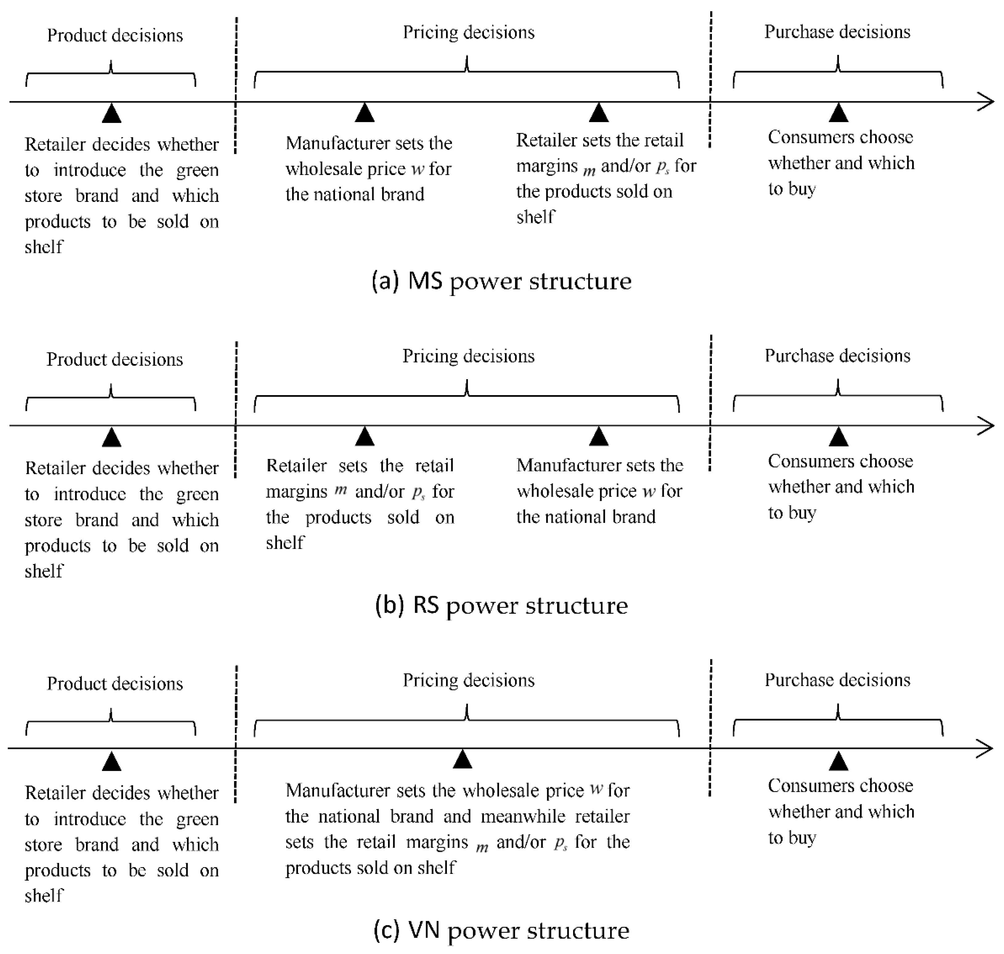
Figure 1. Sequence of Decisions.
Sustainability 14 11995 g001
Figure 2. Retailer’s product strategies under different power structures.
Sustainability 14 11995 g002
Figure 3. Effects of parameters on wholesale prices.
Sustainability 14 11995 g003
Figure 4. Effects of parameters on retail margins of the national brand.
Sustainability 14 11995 g004
Figure 5. Effects of parameters on retail prices of the store brand.
Sustainability 14 11995 g005
Figure 6. Effects of parameters on retail prices of national brand.
Sustainability 14 11995 g006
Figure 7. Effects of parameters on the profits of retailer.
Sustainability 14 11995 g007
Figure 8. Effects of parameters on the profits of manufacturer.
Sustainability 14 11995 g008
Table 1. List of the notations in models.
NotationDefinition
i Subscript, index of brand; i = n for national brand, and i = s for store brand
j Subscript, index of supply chain member; j = M for manufacturer, and j = R for retailer
G Superscript, index of supply chain power structure; G = M S , R S , V N
θ Consumers’ willingness to pay for the unit perceived value
λ Consumers’ green preference
c i Unit cost of product i
w Wholesale price of national brand product
m Retailer’s margin on national brand product
p i Retail price of product i
D i Demand quantity of product i
π j Profit of supply chain member j
Table 2. The optimal solution under different cases.
PS α w G m G p n G p s G D n G D s G π m G π r G
MS ( 0 , 1 2 ] 1 + c n 2 1 c n 4 3 + c n 4 N/A 1 c n 4 0 ( 1 c n ) 2 8 ( 1 c n ) 2 16
( 1 2 , λ 2 λ 1 ) 1 + c s λ λ c s 2 2 λ + c s 2 λ + c s 2 λ c s 2 0 ( 1 + c s λ c n ) ( λ c s ) 2 ( λ c s ) 2 4
( λ 2 λ 1 , λ ) c s + λ c n 2 λ 2 λ c s λ c n 4 λ 2 λ + λ c n + c s 4 λ λ + c s 2 c s λ c n 4 ( λ 1 ) 1 2 + λ c n ( 2 λ 1 ) c s 4 λ ( λ 1 ) ( c s λ c n ) 2 8 λ ( λ 1 ) ( c s λ c n ) 2 + 4 ( λ 1 ) ( λ c s ) 2 16 λ ( λ 1 )
[ λ , + ) N/AN/AN/A λ + c s 2 0 λ c s 2 λ 0 ( λ c s ) 2 4 λ
RS ( 0 , 2 λ 4 ( 2 λ + 1 ) ] 1 + 3 c n 4 1 c n 2 3 + c n 4 N/A 1 c n 4 0 ( 1 c n ) 2 16 ( 1 c n ) 2 8
( 2 λ 4 ( 2 λ + 1 ) , λ 2 ( 2 λ 1 ) ] c n + ( λ 1 ) ( λ c s ) λ 2 2 λ c n + ( 2 1 λ ) c s 1 + c s λ c s λ c s 0 ( λ 1 ) ( λ c s ) 2 λ ( λ c s ) [ 2 ( 1 + c s λ ) c n c s λ ]
( λ 2 ( 2 λ 1 ) , λ 2 λ 1 ] λ 1 + ( 3 λ 1 ) c n 2 ( 2 λ 1 ) 1 c n 2 2 + 3 λ + λ c n 2 ( 2 λ 1 ) λ ( 4 λ 3 + c n ) 2 ( 2 λ 1 ) λ λ c n 2 ( 2 λ 1 ) 0 ( λ 1 ) λ ( 1 c n ) 2 4 ( 1 2 λ ) 2 λ ( 1 c n ) 2 4 ( 2 λ 1 )
( λ 2 λ 1 , λ ) c s + 3 λ c n 4 λ 1 c n 2 2 λ + λ c n + c s 4 λ λ + c s 2 c s λ c n 4 ( λ 1 ) 1 2 + λ c n ( 2 λ 1 ) c s 4 λ ( λ 1 ) ( c s λ c n ) 2 16 λ ( λ 1 ) ( c s λ c n ) 2 + 2 ( λ 1 ) ( λ c s ) 2 8 λ ( λ 1 )
[ λ , + ) N/AN/AN/A λ + c s 2 0 λ c s 2 λ 0 ( λ c s ) 2 4 λ
VN ( 0 , 2 3 ] 1 + 2 c n 3 1 c n 3 2 + c n 3 N/A 1 c n 3 0 ( 1 c n ) 2 9 ( 1 c n ) 2 9
( 2 3 , 2 λ 3 λ 1 ) 1 + c s λ λ c s 2 2 λ + c s 2 λ + c s 2 λ c s 2 0 ( 1 + c s λ c n ) ( λ c s ) 2 ( λ c s ) 2 4
( 2 λ 3 λ 1 , λ ) c s + 2 λ c n 3 λ 3 λ c s 2 λ c n 6 λ 3 λ + 2 λ c n + c s 6 λ λ + c s 2 c s λ c n 3 ( λ 1 ) 1 2 + 2 λ c n ( 3 λ 1 ) c s 6 λ ( λ 1 ) ( c s λ c n ) 2 9 λ ( λ 1 ) 4 ( c s λ c n ) 2 + 9 ( λ 1 ) ( λ c s ) 2 36 λ ( λ 1 )
[ λ , + ) N/AN/AN/A λ + c s 2 0 λ c s 2 λ 0 ( λ c s ) 2 4 λ
Publisher’s Note: MDPI stays neutral with regard to jurisdictional claims in published maps and institutional affiliations.