Energy Conservation for Indoor Attractions Based on NRBO-LightGBM

Abstract

In the context of COVID-19, energy conservation is becoming increasingly crucial to the overwhelmed tourism industry, and the heating, ventilation, and air conditioning system (HVAC) is the most energy-consuming factor in the indoor area of scenic spots. As tourist flows are not constant, the intelligent control of an HVAC system is the key to tourist satisfaction and energy consumption management. This paper proposes a noise-reduced and Bayesian-optimized (NRBO) light-gradient-boosting machine (LightGBM) to predict the probability of tourists entering the next scenic spot, hence adopting the feedforward dynamic adaptive adjustment of the ventilation and air conditioning system. The customized model is more robust and effective, and the experimental results in Luoyang City Hall indicate that the proposed system outperforms the baseline LightGBM model and a random-search based method concerning prediction loss by 5.39% and 4.42%, respectively, and saves energy by 23.51%. The study illustrates a promising step in the advancement of tourism energy consumption management and sustainable tourism in the experimental area by improving tourist experiences and conserving energy efficiently, and the software-based system can also be smoothly applied to other indoor scenic spots.

1. Introduction

There is huge tourism demand in China, as the prevention and control of COVID-19 improve in recent months, the domestic tourism industry has also begun to recover from the recession. According to the report from the World Travel & Tourism Council, the total contribution of tourism to China’s gross domestic product (GDP) and employment in 2020 are 4.5% and 8.8%, respectively [1]. Both the regular tourism requirements from residents and the explosive growth in the number of visitors from other cities have created challenges for the energy consumption management of scenic spots. The tourist experience and energy conservation must be prioritized in order to achieve the sustainable recovery of the tourism economy and to rationalize tourism energy consumption [2,3].

As tourists need to experience a comfortable visit environment, the importance of the HVAC system is substantial in regulating formaldehyde, VOC, CO₂, and PM_2.5, especially for indoor attractions [4]. On the other side, the booming of HVAC’s energy usage is particularly significant, which leads to heavy electric charges and negative environmental impacts. This issue can be relieved by modifying its operation strategy to achieve a balance between tourist satisfaction and minimum energy consumption. Specifically, the indoor air quality and temperature is highly correlated with the number of people in the area, and human flows are measurable by predicting the trajectory of tourists in real-time; thus, the feedforward control of the HVAC system can be performed once the upcoming load is known. It not only reduces the time delay to ensure a satisfactory temperature and air quality in advance, which brings a better experience for tourists but also lowers excessive settings to avoid unnecessary energy consumption.

Benefiting from the rapid development of artificial intelligence and big data, there have been multiple studies for predicting the trajectories of tourism based on tourist behaviors, trajectories’ similarities, and long short-term memory (LSTM) neural networks. In addition to the prediction methods mentioned above, ensemble learning models typically treat the forecast of scenic spot travel trajectory as a classification problem [5]. A summary of related works is presented in

Table 1. Summary of related works. Source: summarized by author.

Methods	Datasets	Limitations
P-DBSCAN clustering [6]	Geotagged photos from Flicker	Prerequisite of posted photos
Metadata processing and P-DBSCAN clustering [7]	Geotagged photos of Hong Kong
Similarities of trajectory graph [8]	Tourist movement data in Italia and geotagged photos	Big data acquisition issue
LSTM neural network [9,10,11,12,13]	Phone call records; tourist car routes; tourism data of Jeju Island, etc.	Overfitting, memory- and time- consuming
Edge computing and multinomial logit model [14]	Tourist preference from questionnaires	The enhanced model exists, sensitive to environmental changes.
Traditional machine learning [15,16]	Tourist’s historical traveling data

below.

Specifically, in the work presented by Leung et al. [6] and Zhong et al. [7], tourists’ behaviors and the potential attractions they are interested in are examined based on the geotagged photos shared on their social media. The feasibility, however, is heavily reliant on the social habits of tourists, and the method does not apply to those who rarely post on media platforms.

Similarities between trajectories on a graph and the spatial–temporal aspect of trajectories have been worked by Moghtasedi et al. [8], and the authors believe a big amount of data is not currently available regarding tourism, thus building a less data-consuming model and concluding that it outperforms the baseline. As a result, there is still a lot of room to improve, if the corresponding data can be collected abundantly.

Besides, there have been several approaches based on the LSTM model [9,10,11,12,13], as an implementation of a recurrent neural network (RNN). Those papers demonstrate similar concepts and appear to achieve higher performance on the dataset than comparative models. There were undeniably strong theoretical achievements to those deep learning methodologies. However, LSTM has a greater probability of overfitting, and its memory consumption and time complexity issue lead to difficulties in applications.

On the other hand, ensemble learning models are also widely adopted. For instance, Deng et al. analyze the destinations of tourists by combing the technology of edge computing and multinomial logit model [14], to calculate the weight value of tourism-destination-selection preference. In another study presented by Zheng et al. [15], the prediction problem is treated by supervised machine learning algorithms named random forests and Lambda Mart. Similar traditional machine learning techniques were applied by Zhao et al. [16], which proposes a tourist arrival forecasting approach based on time-series trajectory similarity using data of tourists’ historical patterns. As the models are trained utilizing data in a specific period, when the external environment changes, the features learned from the original dataset may no longer be applicable, resulting in a decrease in online predictive effectiveness and a significant time-cost associated with the retraining process.

The novelty and new contributions of this paper are the improvements of the difficulties discovered by existing studies on the aspects of data collection, accuracy, and flexibility. Firstly, it optimizes an ensemble learning model that achieves better results compared to the baseline one for a higher accuracy of prediction while simultaneously being able to study the daily latest data to make it up-to-date against environmental changes; it hence conserves more energy by adjusting the HVAC system based on the real-time prediction outcomes. Moreover, the data are collected from various sources and plentiful features are built that contribute to the training of the model, and it also gives the model a capacity to be applied in relatively small areas such indoor attractions, which is more practical, in contrast to other studies that mainly focus on tourists’ flow between large regions.

The rest of the paper is organized as follows. Section 2 demonstrates the methodologies of the research’s approach. Section 3 explains the experiment processes and results, and Section 4 further discusses the results, while simultaneously concluding the paper and illustrating future study directions.

2. Materials and Methods

2.1. System Framework

The three main parts of the system are data processing, model training, and HVAC control. Firstly, concerning data collection, the proposed system uses face-recognition technology to track tourist trajectories and identify their basic attributes such as gender and age, it also gathers scenic spots’ weather and geographic features from the crawler server, and other particulars such as merchants’ payment information are provided by the scenic spots’ managers, followed by data processing and feature engineering. Secondly, the system deploys a noise-reduced and Bayesian-optimized gradient-boosting machine (NRBO-LightGBM) model for offline training; the latest data collected each day is added for training, and the optimal parameters are updated automatically before the scenic spot opens the next day to improve the flexibility and timeliness of the forecast model, so that the trajectory of tourists can be precisely predicted in real-time during the scenic spots’ business hours, hence adjusting the HVAC system based on the number of people in each area. The flow of information between each component comprises the collected raw data being processed and utilized as an input of the model, followed by model training and the output, as the predicted number of tourists can be used to determine the target air volume and temperature, therefore adjusting the HVAC system. The framework of the proposed system is shown in Figure 1.

The system is verified by using real-world data obtained from Luoyang City Hall in China, which is a large cultural tourism complex that contains a tourist service center and eleven distinct indoor scenic spots combining culture, art, entertainment, and shopping.

2.2. Basic LightGBM Model

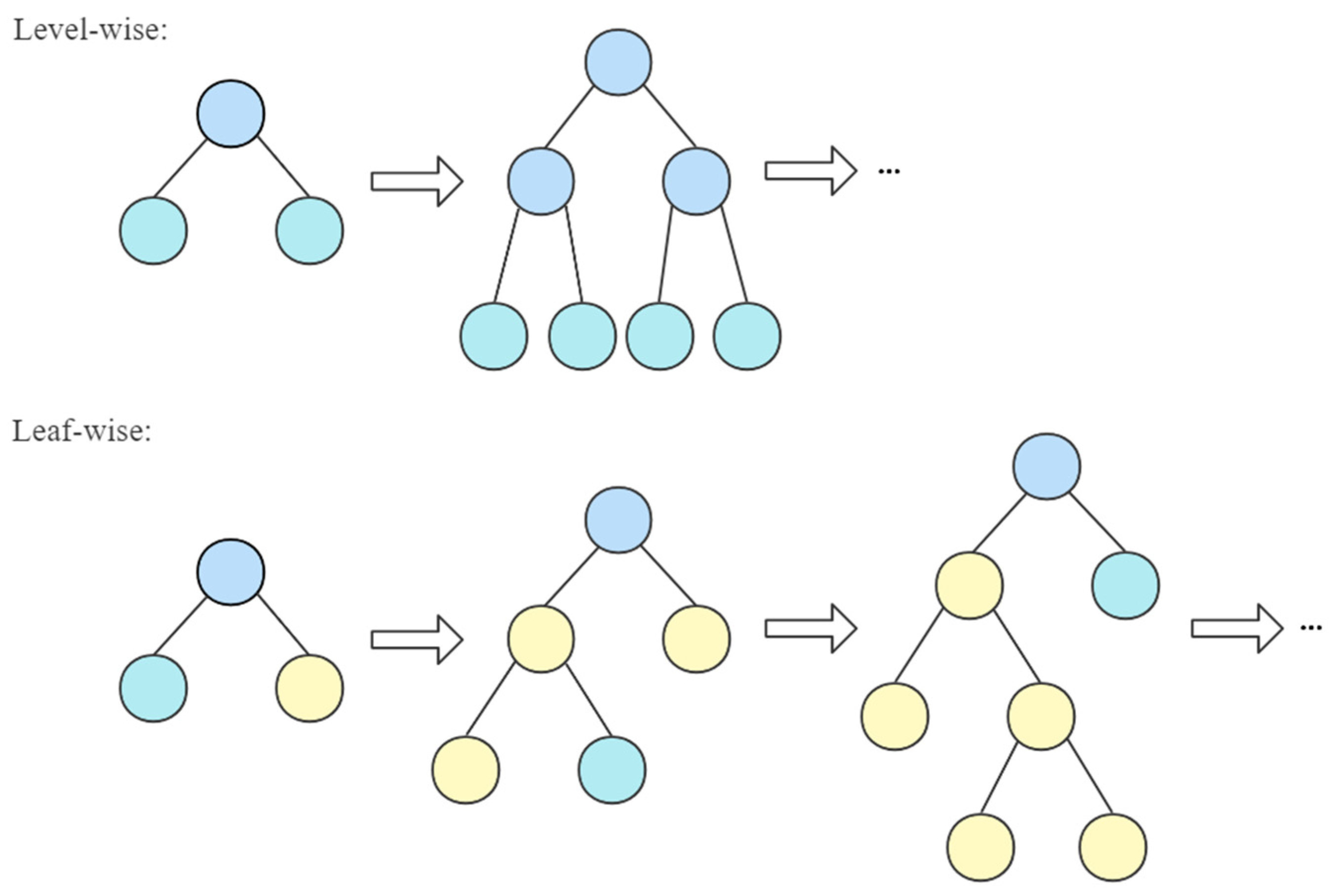
LightGBM is an efficient implementation of gradient-boosting decision trees (GBDT) [17]; it utilizes a leaf-wise growth strategy such that the leaf node with the greatest split gain is selected for growth. Compared to other boosting algorithms, such as XGBoost [18], which adopts the level-wise growth strategy shown in Figure 2, LightGBM can experience lower errors when growing to the same left node, and the depth of tree growth is controlled by hyperparameters to avoid over-fitting.

Moreover, LightGBM uses the gradient-based one-side sampling (GOSS) and exclusive feature bundling (EFB) methods [19]. To be specific, GOSS randomly drops data instances with small gradients and focuses on instances with large gradients, as they contribute more to the computation of information gain, which is more efficient than traversing all instances and provides better accuracy than uniformly random sampling. EFB combines mutually exclusive features into a single feature, which further reduces the algorithm’s time complexity. In addition, LightGBM is based on a histogram algorithm, as can be seen in Figure 3, resulting in a lower memory footprint and higher efficiency.

Improvements in both accuracy and training speed give LightGBM the ability to handle big data regarding scenic tourism. Its objective function consists of a loss function plus a regularized term:

$$ob{j}^{\left(t\right)}={\displaystyle \sum }_{i=1}^{n}l\left(y_i,\widehat{y_i}\right)+{\displaystyle \sum }_{k=1}^K\mathsf{\Omega }\left(f_k\right)$$

(1)

where $y_i$ is the target value, $\widehat{y_i}$ is the predicted value, and $l$ is the loss function. Taylor expansion can be applied to the objective function:

$$ob{j}^{\left(t\right)}={\displaystyle \sum }_{i=1}^n\left[l\left(y_i,{\widehat{y_i}}^{\left(t-1\right)}\right)+g_i{f}_t\left(x_i\right)+\frac{1}{2}{h}_i{f}_t^2\left(x_i\right)\right]+\mathsf{\Omega }\left(f_t\right)$$

(2)

Among:

$$g_i=\frac{\partial l\left(y_i,{\widehat{y}}_i^{\left(t-1\right)}\right)}{\partial {\widehat{y}}_i^{\left(t-1\right)}},h_i=\frac{{\partial }^{2}l\left(y_i,{\widehat{y}}_i^{\left(t-1\right)}\right)}{\partial {\widehat{y}}_i^{\left(t-1\right)}}$$

(3)

As the previous (t−1)th tree is certain when training the t-th tree, $l\left(y_i,{\widehat{y_i}}^{\left(t-1\right)}\right)$ is a constant number, ignoring the constants and substituting the regularization term $\gamma T+\frac{1}{2}\mathsf{\lambda }\sum _{j=1}^T{w}_j^2$ into the objective function then:

$$\begin{array}{l}ob{j}^{\left(t\right)}={\displaystyle {\displaystyle \sum }_{i=1}^n}\left[g_i{f}_t\left(x_i\right)+\frac{1}{2}{h}_i{f}_t^2\left(x_i\right)\right]+\gamma T+\frac{1}{2}\mathsf{\lambda }{\displaystyle {\displaystyle \sum }_{j=1}^T}{w}_j^2\\ ={\displaystyle {\displaystyle \sum }_{j=1}^T}\left[{\displaystyle {\displaystyle \sum }_{i\in I_j}}{g}_i+\frac{1}{2}\left({\displaystyle {\displaystyle \sum }_{i\in I_j}}hi+\mathsf{\lambda }\right)w_j^2\right]+\gamma T\\ ={\displaystyle {\displaystyle \sum }_{j=1}^T}\left[G_j+\frac{1}{2}\left(H_j+\mathsf{\lambda }\right)w_j^2\right]+\gamma T\end{array}$$

(4)

where $w_j$ is the prediction result, taking the derivative of the objective function with respect to $w_j$ yields the optimal $w_j^{*}$ and $ob{j}^{*}$:

$$\begin{array}{c}{w}_j^{*}=-\frac{G_j}{H_j+\mathsf{\lambda }}\end{array}$$

(5)

$$\begin{array}{c}\begin{array}{c}ob{j}^{*}=-\frac{1}{2}{\displaystyle {\displaystyle \sum }_{j=1}^T}\frac{G_j^2}{H_j+\mathsf{\lambda }}+\gamma T\end{array}\end{array}$$

(6)

where $ob{j}^{*}$ is the loss when adding the t-th tree; the smaller the loss is achieved, the better the structure and parameters the t-th tree is trained; hence, the split location of the t-th tree can be determined, and the gain is calculated as:

$$\mathit{Gain}=\frac{1}{2}\left[\frac{G_L^2}{H_L+\mathsf{\lambda }}+\frac{G_R^2}{H_R+\mathsf{\lambda }}-\frac{{\left(G_L+G_R\right)}^2}{H_L+H_R+\mathsf{\lambda }}\right]$$

(7)

where $\frac{G_L^2}{H_L+\mathsf{\lambda }}$ stands for the loss of the left subtree, $\frac{G_R^2}{H_R+\mathsf{\lambda }}$ stands for the loss of right subtree, and $\frac{{\left(G_L+G_R\right)}^2}{H_L+H_R+\mathsf{\lambda }}$ stands for the loss without splitting. The optimal tree structure is obtained by continuously utilizing the gain formula, and the leaf node with the greatest gain can be found for splitting.

2.3. NRBO-LightGBM

2.3.1. Noise Reduction

One of the disadvantages of LightGBM model is widely believed to be the impressionability of the influence of noises, for the reason that it is a boosting method, each iteration of which adjusts the weights of the samples based on the predictions of the previous iteration. As the iterations continue, the error and bias of the model will become smaller. As a result, the bias-based model is more sensitive to noises, and various methods were invented in this paper to address this issue.

Firstly, during the growth of trees in the LightGBM model, the depth of the trees may become too deep, and the model studies the entire training data including the noise and random fluctuations but fail to generalize unseen data scenarios. Although there are several hyperparameter that can be used to limit the max depth of trees and the number of estimators, the loss function of LightGBM was customized by adding L1 regularization rather than L2 regularization, as a large number of features were expected in order to further prevent the risk of over-fitting. L1 regularization is also called least absolute shrinkage and selection operator regression, and it uses shrinkage to obtain the subset of predictors that minimizes prediction error for a quantitative response variable by imposing a constraint on the model parameters that causes regression coefficients for some variables to shrink toward zero. To be specific, the original loss function is as follows:

$$Loss=-\frac{1}{N}{\displaystyle \sum }_{i=1}^{N}L\left(y_i,F_{t-1}\left(x_i;A_{t-1}\right)\right)$$

(8)

where $F_{t-1}\left(x_i;A_{t-1}\right)$ is the prediction of input xi of the model constructed by the t−1th tree with the parameters $A_{t-1}$, which contains the parameters $a_1$, …, $a_{t-1}$ of the t−1th tree. The logarithmic loss function $L\left(y_i,F_{t-1}\left(x_i;A_{t-1}\right)\right)$ indicates the deviation between real value $y_i$ and model’s prediction result. The customed loss function of the t-th tree is:

$$Los{s}_{\mathrm{customed}}=-\frac{1}{N}\left({\displaystyle \sum }_{i=1}^N{\alpha }_{i}L\left(y_i,F_{t-1}\left(x_i;A_{t-1}\right)\right)+\frac{\mathsf{\lambda }}{2}\parallel \alpha \parallel \right)$$

(9)

where $\mathsf{\lambda }$ represents the regularization strength that, as it gets larger, the features’ coefficients are reduced, hence avoiding the over-fitting issue.

Moreover, as the scenario is multi-class classifications, the one-versus-rest technique is applied. The model builds n binary classifiers such that n is the number of classes, and, for each classifier, the class is fitted against all of the other classes. When it comes to the coefficient ${\alpha }_i$ in the customed loss function, it can be denoted as

$${\alpha }_i=\{\begin{array}{c}c,\hspace{0.25em}\hspace{0.25em}\hspace{0.25em}\hspace{0.25em}{y}_i=1\\ 1,\hspace{0.25em}\hspace{0.25em}\hspace{0.25em}\hspace{0.25em}{y}_i=0\end{array}$$

(10)

where $y_i=0$ represents the current class, and $y_i=1$ represents the rest of the classes, and c is a constant depending on the proportion of the sample sizes between the current class and the rest of the classes. By adjusting the sample weight during training, the accuracy when the model studies unbalanced samples can be improved.

2.3.2. Bayesian Optimization

Concerning scenic spots, changes in tourists’ demand and preferences and the adjustments of merchants’ business hours, as well as systematic risks such as typhoons and unexpected pandemics, will cause significant impacts on tourists’ trajectories. Conventional classifiers study feature characteristics from historical data over a period of time, resulting in reduced effectiveness concerning new mutant samples. On the other hand, after adding new data collected daily for training, LightGBM’s various hyperparameters, such as learning rate, number of estimators, regression alpha, etc., will form multiple combinations. Adjusting these parameters manually is usually time-consuming and lacks accuracy, the grid search method supports parallel computing, but meanwhile, memory-consuming random search arbitrarily selects combinations in the search space, which improves efficiency but fails to secure the accuracy of the model [20]. To address this issue, this paper applies Bayesian optimization to automatically seek the optimal parameters for LightGBM.

Bayesian optimization utilizes the theory of approximation and will adaptively design the next round of tuning experiments based on the prior evaluation results of the objective function; it locates the optimal combinations of parameters over iterations using the prior function and the acquisition function [21]. The Bayesian approach eliminates the need for the traversal of all parameter combinations and reduces the exploration space, leading to fewer and faster iterations, as opposed to a grid search. Moreover, prior information is exploited by avoiding parameters that cannot yield good results, making its accuracy superior to random search. A framework of three mainstream Bayesian optimization algorithms can be seen from

Table 2. Bayesian optimization algorithms. Source: summarized by the author.

Algorithms	Prior Function	Acquisition Function	Applicable Scope
BO	Gaussian process	Expected improvement	Low-dimensions
SMAC	Random forest regressor	Upper confidence bound	Discrete variable
TPE	Gaussian process	Expected improvement	High-dimensions

below [22,23,24,25,26,27].

Tourist trajectory prediction is a high-dimensional scenario. In addition to being effective in high-dimensional space, a tree parzen estimator (TPE) improves its speed considerably when compared with other algorithms. The expression of TPE’s acquisition function is:

$$EI(x)=\{\begin{array}{ll}\left({\mu }_t\right(x)-f(x^{+})-ϵ)\Phi \left(Z\right)+{\sigma }_t\left(x\right)\varphi \left(Z\right),\hspace{0.25em}\hspace{0.25em}\hspace{0.25em}\hspace{0.25em}& \mathrm{if} {\sigma }_t\left(x\right)>0\\ 0\hspace{0.25em}\hspace{0.25em}\hspace{0.25em}\hspace{0.25em}& \mathrm{if} {\sigma }_t\left(x\right)=0\end{array}$$

(11)

Among:

$$Z=\frac{{\mu }_t\left(x\right)-f\left(x^{+}\right)-ϵ}{{\sigma }_t\left(x\right)}$$

(12)

where $f\left(x^{+}\right)$ is the current maximum value of the function, $\mathsf{\Phi }\left(Z\right)$ denotes the standard normal cumulative distribution function, $\varphi \left(Z\right)$ denotes the standard normal probability density function, and $ϵ$ is used to balance between exploration and exploitation.

For each x, substituting $f\left(x^{+}\right)$ and ${\sigma }_t\left(x\right)$ derived from a Gaussian process can compute EI and find the x that maximizes EI; hence, the result keeps approaching the minimum value of the loss function. The initial parameters of the TPE algorithm used in the prediction system are set to the present parameters of the model, i.e., the best parameters found by the previous day of training.

2.4. Dynamic Adaptive Adjustment

The minimum fresh air volume is supposed to satisfy people’s hygiene requirements and purify air pollution generated by contaminants such as decoration materials in construction. The strategy to adjust air volume is designed in accordance with the forecast of tourist trajectory. Once the following scenic spots that tourists are most likely to enter are known, the number of people in a scenic area for the next period is also recognizable. Thus, the fresh air volume for people’s hygiene requirements can be calculated by multiplying the predicted tourist flow by fresh air standard per people specified in ASHRAE Standards [28], and the minimum air volume required is:

$$L_{W,min}=L_{p}P+L_{b}A$$

(13)

where $L_p$ is the minimum hourly fresh air required for per people, P is the upcoming number of people in a scenic spot based on trajectory prediction, $L_b$ is the minimum hourly fresh air for construction, and A is the area.

On the other side, ventilation also influences the strategy of air conditioning. The room temperature tolerance is in the range of $T_{min}$ and $T_{max}$, which is the level of indoor temperature that typical individuals can tolerate. When the indoor temperature falls outside the range, the air conditioning system start to work to bring the temperature back to a satisfactory level. However, when the current temperature is less than $T_{min}$ or greater than $T_{max}$, the primary consideration is if ventilation can be utilized. The total ventilation of a single area is assumed to be the sum of $L_{W,min}$ and variable natural ventilations such as open windows, which is in the range of $G_{min}$ and $G_{max}$.

If the indoor temperature $t_{bz}$ is less than $T_{min}$ and the outside temperature $t_o$ is also less than $T_{min}$, the ventilation quantity is set at its minimum level $G_{min}$. In contrast, if the outside temperature is greater than $T_{min}$, the indoor temperature corresponding to $G_{max}$ is calculated as:

$$t_r=\frac{T_{bz}+A\left(G_{max}-G_{min}\right)t_o}{1+A\left(G_{max}-G_{min}\right)}$$

(14)

Consequently, $t_r$ is compared with $T_{min}$; if $t_r$ is less than $T_{min}$, the area still needs heating and ventilation is not appropriate, which is set at $G_{min}$. Moreover, if $t_r$ is greater than $T_{max}$, the ventilation quantity is excessive and should be set at a lower level as:

$$G=\frac{\frac{\left(T_{\mathit{set} min}+T_{\mathit{set} max}\right)}{2}-t_{bz}}{A\left(t_o-\frac{\left(T_{\mathit{set} \mathit{min}}+T_{\mathit{set} max}\right)}{2}\right)}$$

(15)

where indoor temperature will be balanced at:

$$t_r=\frac{\left(T_{set min}+T_{set max}\right)}{2}$$

(16)

Situation where indoor temperature $t_{bz}$ is greater than $T_{max}$ shows the same logic, and the temperature of indoor areas with multiple rooms consists of base temperature and the heat/cooling generated by the air conditioning system can thus be calculated as:

$$t_k(\tau )=t_{k, \mathrm{base} }(\tau )+{{\displaystyle \int }}_{-\infty }^{\tau }{\displaystyle \sum }_{i=1}^n{\phi }_i\ast e^{{\mathsf{\lambda }}_i\ast \left(\tau -\eta \right)}\ast q(\eta )\ast d\eta +{{\displaystyle \int }}_{-\infty }^{\tau }{\displaystyle \sum }_{j\in adj}{\displaystyle \sum }_{i=1}^n{\phi }_{ij}\ast e^{{\mathsf{\lambda }}_i\ast \left(\tau -\eta \right)}\ast q_j(\eta )\ast d\eta$$

(17)

where $t_k(\tau )$ is the temperature of area k; $t_{k, \mathrm{base} }(\tau )$ is the base temperature of area k; $q(\eta )$ is the adjacent thermal disturbances between areas including the influence of adjacent areas’ temperatures on area k through heat transfer as $t_j(\tau )-t_{j, \mathrm{base} }(\tau )$ and the influence through mutual exchange of air as $G_{jk, \inf }·\left(\left(t_j(\tau )-t_{j, \mathrm{base} }(\tau )\right)-\left(t_k(\tau )-t_{k, \mathrm{base} }(\tau )\right)\right)$; $q_j$ is the thermal disturbance in area, which is mainly caused by the number of people in this area for the next period predicted by NRBO-LightGBM; ${\mathsf{\lambda }}_i$ is the vector of spatial eigenvalues for each area under the state-space method; ${\phi }_{ij}$ is the coefficient of influence of various disturbances on room temperature after sampling; n is the dimensionality of the eigenvalues of various heat disturbances; and adj is a set of heat disturbances belonging to adjacent rooms.

As a result, the HVAC system can adjust its ventilation and air conditioning strategies dynamically adaptively to the trajectory prediction results based on NRBO-LightGBM in order to conserve energy.

2.5. Data Analysis

2.5.1. Data Collection

In order to improve the problems regarding data acquisition, the cameras are deployed to capture video stream data and convert it into picture frames in real-time, hence converting it to a matrix to obtain basic attributes such as gender, age, and other character portraits, combined with consumer information to capture visitors’ payment data, and to further obtain tags for social attributes such as interest preferences and spending power based on a historical analysis of that visitor. A real-time monitor of the tourist distribution in each site is shown in Figure 4 below.

Moreover, payment data can be used to gain knowledge about the commodities prices, orders, and quantities of merchants in the scenic area. Weather information of the scenic spot is obtained through a crawler server to form time-stamped features such as temperature, humidity, and rainfall probability. Tourist historical trajectories are also recorded in the form of a time series, while the flow tendency features, as well as scenic spot geographic location features, are included as a part of the metadata. The model predicts scenic spots by labeling them with numbers from 0 to 11.

In addition, the locations and specifications of air conditioning units, as well as historical energy consumption data, are supported directly by the manager of Luoyang City Hall.

2.5.2. Data Processing and Feature Engineering

The original dataset is the combined data from March 2020 to November 2021 gathered in Luoyang City Hall; after stratified sampling, it has a total of 26,750 rows and 28 eigenvalues. Due to the variabilities in sizes, popularities, and other characteristics of different scenic spots, the number of tourists may vary by tens of times, and there exist issues of imbalanced labels, as is shown in Figure 5.

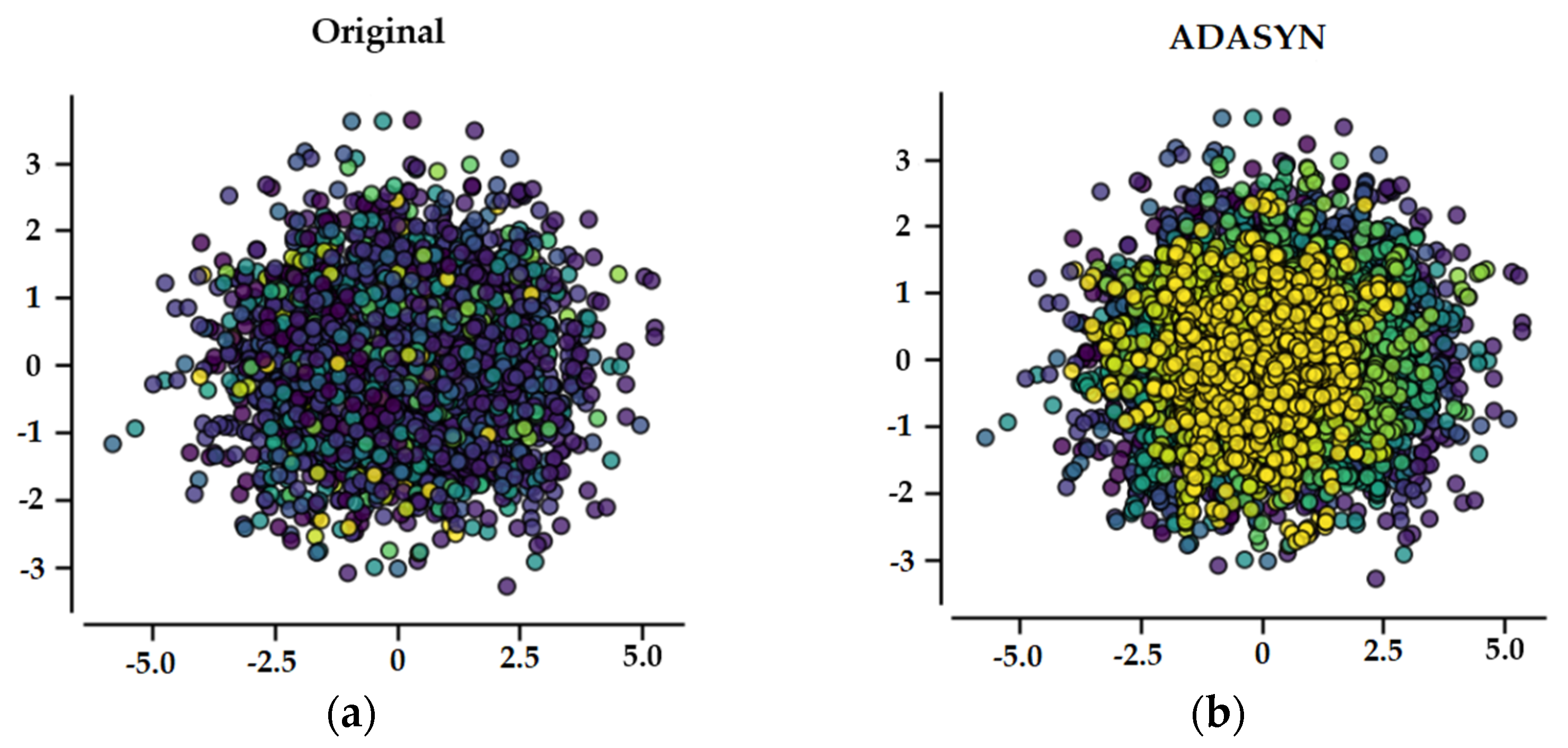
Imbalanced classifications will induce prediction results to be biased towards the category with more observations. Therefore, the adaptive synthetic (ADASYN) sampling method was chosen to analyze and simulate the classes with low proportions of samples [29]. During the simulation, a weighted distribution of K nearest neighbors and the distributions of minority class samples are calculated according to the learning difficulties of the data, wherein the number of data synthesized has a positive relationship with the learning difficulties. The scenic spot with the highest number of labels is used as the benchmark, which is 6703 in this case, and, for scenic spots with labels less than 1/10 of the benchmark, new samples are synthesized by the ADASYN algorithm to increase its proportions to reach 1/10, thus solving the imbalance problem without changing the data distribution essentially. The dataset became 28,717 rows after over-sampling, and the layout of total samples is presented in Figure 6.

Consequently, deduplication was performed, followed by filling missing values such that continuous features were filled with means and medians based on their distributions, and discrete features were filled by the value with the highest frequency. As tourism is cyclical, the outliers of low and peak seasons are treated separately. In the low seasons, visitors are mainly supported by the regular travel demand of residents and outliers are tested and deleted using PauTa Criterion [30]. On the other hand, in peak seasons, the area may experience a sudden increase in the number of visitors but with a historical cyclical pattern, which is monitored by Facebook’s time-series data prediction algorithm ‘Prophet’ [31]. Non-numerical labels were transferred to numerical ones, while long-tail data were classified as ‘others’ to avoid the curse of dimensionality. Hourly temporal information was extracted from timestamps and binned into groups. A scenic spot’s popularity is measured by the historical trajectory of tourists, as well as their duration of stay. In addition, attributes related to business are computed, such as by multiplying the price of goods by quantity to obtain the total sales of goods; generic features including statistical features, ratio features, and ranking features were also constructed.

The feature selection method is based on random forest [32]. For each decision tree, the corresponding out-of-bag error is calculated as errOOB1, and errOOB2 is calculated after randomly adding noise interference to feature X of all samples in the out-of-bag data. Assuming there is a total of N trees, the importance of feature X is:

$$RFfi={\displaystyle \sum }_1^N\left(\mathrm{errOOB}2-\mathrm{errOOB}1\right)/ \mathrm{Ntree}$$

(18)

A substantial increase in the out-of-bag error indicates a high level of feature importance, and a maximum limit of 80 features was set in order to achieve a computational efficiency that meets the need for timeliness.

3. Results

This section first presents an introduction of the experimental area, then details the prediction process concerning data and model training. Various aspects regarding the results of trajectory prediction and energy consumption are discussed. The implementations were operated on a machine with an Intel i5-10400 2.9 GHz six-core central processing unit (CPU), 16G random access memory (RAM), and Python was used for programming.

3.1. Experimental Area

Luoyang City Hall is located at the Luoyang International Convention and Exhibition Center in Henan, China; it has a total area of 24,000 m², with one tourist service center and eleven attractions, including the Artisan Elegance Collection, Internet Experience Hall, Art Hall, Cultural Display Gallery, Wax Museum, Peony Flower Gallery, and Heritage Street, etc. In the scenic spot, there are various types of businesses, such as catering, photography, ceramics, jade, and virtual reality, as can be seen from Figure 7 in the ichnography of Luoyang City Hall. As an iconic cultural and tourism facility in Luoyang, Luoyang City Hall attracts visitors mainly from cities in Henan Province, such as Luoyang, Zhengzhou, and Kaifeng, as well as tourists from neighboring provinces, such as Shandong and Jiangsu. As all of the attractions at Luoyang City Hall are indoor and have built-in air conditioning units, it is an ideal place to examine the effectiveness and value of the prediction and energy-saving system.

3.2. Model Training

The NRBO-LightGBM model was trained in comparison with a baseline model that uses the default parameters, as well as a random-search-optimized LightGBM model. The models were subjected to 5-fold cross-validation by randomly splitting the data into five groups, each comprising 20% of the data, and using as the test set for one of the five validations, while the remaining 80% of the four groups of data were used as the training set. To some extent, this can further reduce potential overfitting problems and lead to more reliable results.

3.3. Trajectory Prediction Results

The LightGBM baseline model obtained a minimum loss of 0.6311, while the minimum loss of the model under random search is 0.6247, and the noise-reduced model under Bayesian optimization using TPE achieved a lower loss of 0.5971. The top five rounds of the training ordered by loss in ascending rank are present in

Table 3. Top 5 best results obtained by NRBO and random search. Source: compiled on the basis of the author’s experimental results.

Rank	NRBO Loss	NRBO Time	RS Loss	RS Time
1	0.597118	1.036272	0.624709	0.778372
2	0.597160	0.804573	0.624742	0.818155
3	0.597161	0.769298	0.62475	0.754016
4	0.597163	0.778566	0.624757	0.711813
5	0.597171	0.775609	0.624762	0.70055

.

The results show that the proposed method outperforms the baseline and the random-search-based LightGBM model by 5.39% and 4.42%, respectively. On the other hand, it takes a total of 253.8 s for the NRBO LightGBM model to finish training, which is slightly longer but on the same level compared with 246.2 s of the random search method. The contrastive training time of each round is presented in Figure 8 below.

To further understand the logic behind the algorithms, the variation of parameters throughout the training process is explored. The key optimal hyperparameters of the three different methods corresponding to the minimum loss can be seen from

Table 4. Key optimal hyperparameters. Source: compiled on the basis of the author’s experimental results.

Parameters	Baseline (Default)	Random Search	NRBO
learning_rate	0.1	0.08	0.13
n_estimators	20	59	49
num_leaves	31	68	150
reg_alpha	0	0.57	0.09
subsample_for_bin	200,000	180,000	200,000

.

The proposed method tends to have more advantages in the phase of fitting optimal results. For instance, the distributions of the parameter concerning the number of leaves are illustrated in Figure 9. It is noticeable that the distribution of NRBO-LightGBM focuses on the best parameter with a higher density than the random search method.

Moreover, when it comes to the loss, the characteristic of seeking advantages on prior information leads to results concentrating near the optimal solution and skew to the right, while the loss of random search approximates the normal distribution, as it can be seen from Figure 10 below.

A stress test was also performed by scaling the sample size of the training set up to 2 million, and a five-hour training time met the expectations of daily training and updating optimal parameters. In addition, it only took 1.2 s to predict a sample of 4000 visitors online that satisfied the requirement of real-time predictions.

3.4. Energy Consumption Comparison

The fresh air volume control method currently adopted by the manager of the experimental area is based on the time-series algorithm ‘Prophet’ such that the upper bound of the forecast range of a day’s average tourist flow is used to set the air volume constantly throughout the day. As the construction type of Luoyang City Hall belongs to the category of the exhibition hall, the minimum fresh air volume for people’s hygiene requirements according to China’s public construction energy-saving-design standard (GB50189-2005) is 20 m³/(h × p), and the minimum fresh air volume for construction is 0.9 m³/(h × m²). The comparison of target air volume between the proposed method and the time-series-based method of a typical hour of midday in December 2021 is shown in

Table 5. Target air volume of Luoyang City Hall. Source: compiled on the basis of the author’s experimental results.

Scenic Spot	People	Proposed $({\mathbf{m}}^3/\mathbf{h})$	People *	Time Series $({\mathbf{m}}^3/\mathbf{h})$
Wax Museum	231	6971.68	265	7651.68
Culture and Creative Museum	183	5544.48	233	6544.48
Library	74	2792.42	122	3752.42
Art Museum	98	3116.02	130	3756.02
Internet Experience Hall	145	4299.87	159	4579.87
Artisan Elegance Collection	84	4367.33	104	4767.33
Studio Hall	76	2937.59	110	3617.59
Cultural Display Gallery	144	4312.84	160	4632.84
Heritage Street	98	3280.42	136	4040.42
Peony Flower Gallery	242	7485.30	276	8165.30
Gift Institute	83	2619.96	133	3619.96
Tourist Service Center	26	1025.30	38	1265.30
Total	1484	48,753.21	1866	56,393.21

* Upper limit of daily average people flow forecasted by FBProphet.

.

The hourly total expected target average air volume of the proposed method is 48,753.21 m³/h, which is 13.55% less than the 56,393.21 m³/h of the other approach, and still ensures a satisfactory level of air standard. Similarly, the corresponding indoor temperatures are calculated, and the operations of the air conditioning system are regulated. The result of total energy consumption is shown in Figure 11, which indicates a daily energy saving of 23.51% due to the flexible adjustment of air volume according to the trajectory predictions. On the other hand, the time-series method set the air volume in reference to the maximum forecast number of people; thus, its energy consumption appears to be constant in general and is fundamentally larger.

4. Discussion

With a detailed research on tourism energy conservation techniques, the experimental results demonstrate that the NRBO-LightGBM model developed in this paper is superior to its competitors such as ‘Prophet’. The phenomenon can also be interpreted by the algorithms’ underlying logic. Specifically, although the time-series-based algorithm ‘Prophet’ is capable of dealing with periodic data, even catching holiday trends, its outcome is a range that shows the daily minimum and maximum predicted number of tourists. As a result, the managers have no choice but to adjust the HVAC system according to the maximum number of predicted tourists in each scenic area in order to insure a satisfactory air and temperature level. In real cases, the number of tourists can hardly reach its peak level throughout the day, hence it is not as energy-efficient as the proposed method in the paper, no matter how seasons and trends of tourists change.

To conclude, this paper proposes an innovative tourist trajectory prediction and energy-saving system for indoor attractions based on an improved LightGBM model named NRBO-LightGBM, such that the loss function and coefficient are customized to achieve a higher robust level regarding noises and utilized Bayesian optimization to automatically seek the optimal parameters on a daily basis. It aims to counter the mutable characteristics of tourism; hence, the feedforward dynamic adaptively adjusts the HVAC system in both ventilation and air conditioning, reducing the time delay and minimizing energy consumption. Experimental results regarding Luoyang City Hall demonstrate that the proposed methodology is able to train the daily latest data against environmental changes. It not only achieves 5.39% and 4.42% lower loss compared to the baseline LightGBM and random search approaches, respectively, but also experiences an energy-saving of 23.51%. Therefore, the application of this technology can contribute to tourism energy consumption management and sustainable tourism by improving the tourist experience and conserving energy efficiently in scenic spots.

Moreover, to the best of the authors’ knowledge, this paper is the first to examine trajectories inside a scenic location and profit from the effort of the data-collection part of the prediction system. It is capable of distinguishing tourists between various instructions in a specific scenic spot. In stark contrast to previous studies that focused on tourist trajectories in a relatively large area, such as a city, an island, or even between nations, the proposed system has more practical value and is easier to apply to other indoor attractions.

Future research may focus on a deeper analysis of the popular visit routes of tourists, combined with public sentiments by natural language processing to further improve the performance of model, and the characteristics of people with distinct preferred tour routes will be analyzed to help the shops in scenic spots generate more sales.

References

1. World Travel & Tourism Council. Available online: https://wttc.org/Research/Economic-Impact (accessed on 10 January 2022).
2. Zhang, L.; Zhang, J. A systematic review on tourism energy consumption, sustainable tourism, and destination development: A behavioral perspective. In Transport and Energy Research; Elsevier: Amsterdam, The Netherlands, 2020; pp. 295–313. [Google Scholar]
3. Breiby, M.A.; Duedahl, E.; Øian, H.; Ericsson, B. Exploring sustainable experiences in tourism. Scand. J. Hosp. Tour. 2021, 20, 335–351. [Google Scholar] [CrossRef]
4. Huang, K.; Sun, W.; Feng, G.; Wang, J.; Song, J. Indoor air quality analysis of 8 mechanically ventilated residential buildings in northeast China based on long-term monitoring. Sustain. Cities Soc. 2020, 54, 101947. [Google Scholar] [CrossRef]
5. Egger, R. Machine Learning in Tourism: A Brief Overview. In Applied Data Science in Tourism; Springer: Cham, Switzerland, 2022; pp. 85–107. [Google Scholar] [CrossRef]
6. Leung, R.; Vu, H.Q.; Rong, J.; Miao, Y. Tourists visit and photo sharing behavior analysis: A case study of Hong Kong temples. In Information and Communication Technologies in Tourism; Inversini, A., Schegg, R., Eds.; Springer: Cham, Switzerland, 2016; pp. 197–209. [Google Scholar]
7. Zhong, L.; Yang, L.; Rong, J.; Kong, H. A Big Data Framework to Identify Tourist Interests Based on Geotagged Travel Photos. IEEE Access 2020, 8, 85294–85308. [Google Scholar] [CrossRef]
8. Moghtasedi, S.; Muntean, C.I.; Nardini, F.M.; Grossi, R.; Marino, A. High-Quality Prediction of Tourist Movements Using Temporal Trajectories in Graphs. In Proceedings of the 2020 IEEE/ACM International Conference on Advances in Social Networks Analysis and Mining (ASONAM), Hague, The Netherlands, 7–10 December 2020; pp. 348–352. [Google Scholar]
9. Crivellari, A.; Beinat, E. LSTM-Based Deep Learning Model for Predicting Individual Mobility Traces of Short-Term Foreign Tourists. Sustainability 2020, 12, 349. [Google Scholar] [CrossRef]
10. Mikhailov, S.; Kashevnik, A. Car Tourist Trajectory Prediction Based on Bidirectional LSTM Neural Network. Electronics 2021, 10, 1390. [Google Scholar] [CrossRef]
11. Shafqat, W.; Byun, Y.-C. A Context-Aware Location Recommendation System for Tourists Using Hierarchical LSTM Model. Sustainability 2021, 12, 4107. [Google Scholar] [CrossRef]
12. Crivellari, A.; Beinat, E. Identifying Foreign Tourists’ Nationality from Mobility Traces via LSTM Neural Network and Location Embeddings. Appl. Sci. 2019, 9, 2861. [Google Scholar] [CrossRef]
13. Xu, Y.; Zou, D.; Park, S.; Li, Q.; Zhou, S.; Li, X. Understanding the movement predictability of international travelers using a nationwide mobile phone dataset collected in South Korea. Comput. Environ. Urban Syst. 2022, 92, 101753. [Google Scholar] [CrossRef]
14. Deng, B.; Xu, J.; Wei, X. Tourism Destination Preference Prediction Based on Edge Computing. Mob. Inf. Syst. 2021, 2021, 5512008. [Google Scholar] [CrossRef]
15. Zheng, S.; Liu, Y.; Ouyang, Z. A machine learning-based tourist path prediction. In Proceedings of the International Conference on Cloud Computing and Intelligence Systems (CCIS), Beijing, China, 17–19 August 2016; pp. 38–42. [Google Scholar]
16. Zhao, E.; Du, P.; Sun, S. Historical pattern recognition with trajectory similarity for daily tourist arrivals forecasting. Expert Syst. Appl. 2022, 203, 117427. [Google Scholar] [CrossRef]
17. Friedman, J.H. Greedy function approximation: A gradient boosting machine. Ann. Stat. 2001, 29, 1189–1232. [Google Scholar] [CrossRef]
18. Chen, T.; He, T.; Benesty, M.; Khotilovich, V.; Tang, Y.; Cho, H.; Chen, K. Xgboost: Extreme gradient boosting. In R Package Version 0.4-2; R Foundation for Statistical Computing: Vienna, Austria, 2015; Volume 1, pp. 1–4. [Google Scholar]
19. Ke, G.; Meng, Q.; Finley, T.; Wang, T.; Chen, W.; Ma, W.; Ye, Q.; Liu, T.Y. Lightgbm: A highly efficient gradient boosting decision tree. In Proceedings of the Advances in Neural Information Processing Systems, Long Beach, CA, USA, 4–9 December 2017; p. 30. [Google Scholar]
20. Liashchynskyi, P.; Liashchynskyi, P. Grid search, random search, genetic algorithm: A big comparison for NAS. arXiv 2019, arXiv:1912.06059. [Google Scholar]
21. Letham, B.; Karrer, B.; Ottoni, G.; Bakshy, E. Constrained Bayesian Optimization with Noisy Experiments. Bayesian Anal. 2017, 14, 495–519. [Google Scholar] [CrossRef]
22. Brochu, E.; Cora, V.M.; De Freitas, N. A tutorial on Bayesian optimization of expensive cost functions, with application to active user modeling and hierarchical reinforcement learning. arXiv 2010, arXiv:1012.2599. [Google Scholar]
23. Bergstra, J.; Bardenet, R.; Bengio, Y.; Kégl, B. Algorithms for hyper-parameter optimization. In Proceedings of the Advances in Neural Information Processing Systems, Granada, Spain, 12–15 December 2011; p. 24. [Google Scholar]
24. Wu, J.; Chen, X.Y.; Zhang, H.; Xiong, L.D.; Lei, H.; Deng, S.H. Hyperparameter optimization for machine learning models based on Bayesian optimization. J. Electron. Sci. Technol. 2019, 17, 26–40. [Google Scholar]
25. Cui, W.; Cao, G.; Park, J.H.; Ouyang, Q.; Zhu, Y. Influence of indoor air temperature on human thermal comfort, motivation and performance. Build. Environ. 2013, 68, 114–122. [Google Scholar] [CrossRef]
26. Perrone, V.; Shen, H.; Seeger, M.W.; Archambeau, C.; Jenatton, R. Learning search spaces for Bayesian optimization: Another view of hyperparameter transfer learning. In Proceedings of the Advances in Neural Information Processing Systems, Vancouver, BC, Canada, 8–14 December 2019; p. 32. [Google Scholar]
27. Dong, H.; He, D.; Wang, F. SMOTE-XGBoost using Tree Parzen Estimator optimization for copper flotation method classi-fication. Powder Technol. 2020, 375, 174–181. [Google Scholar] [CrossRef]
28. Ventilation for Acceptable Indoor Air Quality. Available online: https://www.ashrae.org/File%20Library/Technical%20Resources/Standards%20and%20Guidelines/Standards%20Addenda/62-2001/62-2001_Addendum-n.pdf (accessed on 22 January 2022).
29. Alhudhaif, A. A novel multi-class imbalanced EEG signals classification based on the adaptive synthetic sampling (ADASYN) approach. PeerJ Comput. Sci. 2021, 7, e523. [Google Scholar] [CrossRef]
30. Wan, F.; Guo, G.; Zhang, C.; Guo, Q.; Liu, J. Outlier Detection for Monitoring Data Using Stacked Autoencoder. IEEE Access 2019, 7, 173827–173837. [Google Scholar] [CrossRef]
31. Taylor, S.J.; Letham, B. Forecasting at scale. Am. Stat. 2018, 72, 37–45. [Google Scholar] [CrossRef]
32. Breiman, L. Random forests. Mach. Learn. 2001, 45, 5–32. [Google Scholar] [CrossRef] [Green Version]
Figure 1. The framework of the proposed system. Source: author’s development.
Sustainability 14 11997 g001
Figure 2. Level-wise and leaf-wise growth strategy. Source: build on the nature of the algorithm.
Sustainability 14 11997 g002
Figure 3. Histogram algorithm. Source: build on the nature of the algorithm.
Sustainability 14 11997 g003
Figure 4. Real-time tourist distribution. Source: author’s development.
Sustainability 14 11997 g004
Figure 5. Number of samples in each label. Source: compiled on the basis of author’s calculations.
Sustainability 14 11997 g005
Figure 6. The effect of over-sampling: (a) original dataset; (b) dataset after ADASYN over-sampling. Source: compiled on the basis of author’s calculations.
Sustainability 14 11997 g006
Figure 7. Tourists in the ichnography of experimental area. Source: author’s development.
Sustainability 14 11997 g007
Figure 8. The training time of LightGBM under NRBO and random search. Source: compiled on the basis of the author’s experimental results.
Sustainability 14 11997 g008
Figure 9. Distributions of parameters under NRBO and random search. Source: compiled on the basis of the author’s experimental results.
Sustainability 14 11997 g009
Figure 10. Comparison between NRBO and random search: (a) loss distribution under NRBO; (b) loss distribution under random search. Source: compiled on the basis of the author’s experimental results.
Sustainability 14 11997 g010
Figure 11. Energy consumption comparison. Source: compiled on the basis of the author’s experimental results.
Sustainability 14 11997 g011