Abstract
With the increasingly competitive environment in the steel market and the proposed dual carbon goals, the government will need to consider many factors, such as the realization of energy conservation and emission reduction targets, the production game between enterprises, and the adjustment of production strategies of enterprises. Therefore, this research constructs a repeated dynamic game model including carbon trading policy and other mixed reduction policies, introduces a bounded rationality output adjustment strategy, and studies the response, stability, and complexity of different scenarios in the steel industry. The results are as follows: (1) With the gradual increase in emission reduction targets, the output adjustment policies that enterprises can implement will show an increasing trend under the single carbon trading policy. (2) Under the mixed emission reduction policy, the output adjustment policies that affect enterprises with larger outputs will show an increasing trend when targets continue to increase. (3) Smaller-output enterprises will be restricted and affected by more factors, such as emission reduction targets and larger output enterprises. (4) The influence of carbon trading benchmarks on market stability region is not obvious. In summary, enterprises should comprehensively consider emission reduction policies, output adjustment policies, carbon trading benchmarks, and other factors to ensure that the enterprises and the entire market will not fall into an imbalanced state.
1. Introduction
As the most important core industrial sector in China, the iron and steel industry (hereinafter referred to as the steel industry) is an important basic industry of the national economy, an important support for building a modern power country, and an important field for achieving green and low-carbon development. In January 2022, the Ministry of Industry and Information Technology, the National Development and Reform Commission, and the Ministry of Ecology and Environment jointly issued the “Guiding Opinions on Promoting the High Quality Development of the Iron and Steel Industry” (hereinafter referred to as the Opinions), which pointed out that during the “Fourteenth Five Year Plan” period (2021–2025), China’s steel industry still faced problems, such as excess capacity pressure, insufficient industrial safety assurance capacity, low levels of green and low-carbon development, and low industrial concentration.
In particular, with the proposal of the “double carbon” goal, the green and low-carbon development of the steel industry has become a key concern. The government and academia have conducted a lot of research and analysis in formulating industrial emission reduction goals, scientific and technological innovation, and carbon reduction technology. At the same time, the Opinions pointed out that the government will support the construction of a carbon emission data management system in the whole process of steel production and will participate in national carbon emission trading. This means that the issue of the carbon emissions trading and the design of carbon trading mechanisms will become an important task for the development of the steel industry during the 14th Five Year Plan period, and the corresponding mechanism design and policy analysis will also become a research hotspot.
In addition, compared with the description of the steel industry development plan during the 13th Five Year Plan period (2016–2020), the Opinions posited that industrial market safety will be a new challenge for the steel industry. This means that the high-quality development of the steel industry and enterprises should not only strive to solve the problems of innovation ability, industrial structure, green low-carbon, and quality improvement, but also that the safety and stability of the overall steel market will become an important task for the development of the steel industry during the 14th Five Year Plan period. The steel market is composed of various steel production enterprises and, especially in the process of large-scale merger and reorganization of the steel industry and elimination of backward production capacity, the production decisions of steel enterprises will affect the stability of the market to a certain extent. Once the production decision-making of an enterprise is deviated, it will also affect the economic benefits, product output, environmental pollution, and many other aspects of the enterprise and the steel market. Therefore, the production decision-making of an enterprise and the game between enterprises are also worthy aspects of future research.
Obviously, with the introduction of the high-quality development policy for the steel industry, the emission reduction target will be more and more strictly enforced, and the production and trade environment of the steel market will be more complex in the future. In order to ensure the high-quality and sustainable development of the steel industry, it is necessary to consider both the government and enterprises, and also to examine the interest relationship between the government and enterprises and between enterprises. For government departments, it is important to determine how to design a reasonable carbon trading mechanism and emission reduction strategy, and how to maintain the overall stability of the market; for enterprises, it is important to determine how to adjust their production strategies according to the emission reduction goals and achieve high-quality and sustainable development; these will become the main goals and tasks of the steel industry during the 14th Five Year Plan period and even in the medium- and long-term in the future, and these will also be the key issues to be solved by this study and subsequent relevant research.
2. Literature Review
2.1. Generation and Development of Carbon Trading Mechanism
Carbon trading is a general term for greenhouse gas emissions trading. The basic principle is that one party to the contract obtains GHG emission reduction credits by paying the other party, and the buyer can use the purchased emission reduction credits to mitigate the greenhouse effect to achieve its emission reduction goal. Among the six greenhouse gases that are required to be reduced, carbon dioxide (CO2) is the largest, so this transaction is calculated per ton of CO2 equivalent (t CO2 e); thus, it is commonly called “carbon trading”. The United Nations Intergovernmental Panel on Climate Change adopted the United Nations Framework Convention on Climate Change on 9 May 1992. In December 1997, the first additional agreement to the Convention, the Kyoto Protocol (referred to as the Protocol), was adopted in Kyoto, Japan. The “Protocol” regards the market mechanism as a new way to solve the greenhouse gas emission reduction problem represented by CO2, that is, the CO2 emission rights are regarded as a commodity, thus, forming the trading of CO2 emission rights.
The “Protocol” stipulates the quantitative emission reduction targets for countries in Annex I of the United Nations Framework Convention on Climate Change; that is, between 2008 and 2012, their greenhouse gas emissions will be reduced by an average of 5.2% from the 1990 level. Other rules are derived from the “Protocol”. For example, the “Protocol” stipulates that the EU’s collective emission reduction target is 8% lower than the 1990 emissions level by 2012, and that the EU can redistribute it to the member states. The EU took the lead in establishing the EU Emissions Trading System (EU ETS) in 2005, which established trading rules and is the largest carbon market to date. Currently, there are more than 20 carbon emission trading systems in operation around the world. These include the New Zealand carbon emissions trading system established in 2008, the Tokyo carbon trading system established in 2010, the California carbon emissions cap and trading plan established in 2013, the Canada Quebec carbon emissions cap and trading plan established in 2013, and the South Korea’s carbon emissions trading system established in 2015.
According to the “United Nations Framework Convention on Climate Change”, before 2020, China, as a developing country, will not undertake the emission reduction in the legally binding absolute total amount of greenhouse gases. Therefore, although China designated Beijing, Shanghai, Guangdong, Shenzhen, Hubei, Chongqing, and other places as pilot carbon emission trading pilots in 2011, the results were minimal. The main reason is that China’s carbon emission base is not large, and the environmental protection awareness of enterprises is not strong. Around 2015, China’s per capita carbon emissions surpassed that of the European Union, and its total carbon emissions became the world’s largest, which made relevant departments begin to carefully consider the design and implementation of various emission reduction mechanisms, including the carbon tax and carbon trading.
In recent years, China’s total carbon emissions have gradually climbed to the peak, and enterprises are also facing a critical period of transformation and development. If they fail to make good use of this time period, enterprises will not only face high carbon emission quota fees and energy conservation and emission reduction fees, but may also face setbacks in exports due to high emissions. Therefore, the implementation of the necessary emission reduction policies is imminent. Fortunately, as an emission reduction method that has been successfully applied abroad, carbon trading has been promoted in China. On 16 July 2021, the national carbon emissions trading market began online trading. The power generation industry became the first industry to be included in the national carbon market, with more than 2000 key emission units included. China’s carbon market will become the largest market covering greenhouse gas emissions in the world, but other industry sectors have not yet been included in the carbon market.
2.2. Literature Review of Carbon Trading Mechanism in the Steel Industry
As mentioned above, as a more mature emission reduction policy, carbon trading policy has been carried out and implemented in foreign countries for many years, and relevant theoretical research results are constantly emerging. Although China has not yet fully implemented the carbon trading policy, it has also conducted a lot of research on its mechanism design, influencing factors, and multiple emission reduction scenarios. According to the research object and research background of this paper, this paper selects the research literature on carbon trading policy of the steel industry, as follows.
In foreign research, Smale et al. [1] discussed the impact of carbon trading on the competitiveness of enterprises by taking five energy-intensive industries, such as the steel industry and cement industry, as examples in the UK. Allevi et al. [2] analyzed the impact of the EU Emission Trading System (EU ETS) and other policies aimed at reducing carbon emissions and improving the efficiency of production processes on the production choices of the European energy and industrial sectors. Boutabba and Lardic [3] analyzed the impact of EU carbon trading policies on net imports of the EU cement and steel industries, as well as the impact of carbon leakage and loss of competitiveness. In order to understand whether emissions trading will lead to local aggregation of emissions changes, Stuhlmacher et al. [4] conducted a systematic spatial economic assessment of the EU ETS. Hanclova et al. [5] identified and evaluated the interaction between EU ETS factors (prices of emission allowances and grandfathering) and the steel industry factors of the Czech Republic (such as price and output). Karali et al. [6] analyzed the roles of energy efficiency measures, steel commodity, and international carbon trading in achieving specific CO2 emission reduction targets in the US iron and steel sector from 2010 to 2050. Yamazaki [7] examined whether the absolute amount of steel scrap used in Japan increases under an emissions trading scheme using the computable general equilibrium model (CGE model). Kushwaha et al. [8] took Indian steel manufacturers as an example to study the impact of the timing of the implementation of carbon quotas and carbon trading policies on the selection of waste steel collection channels in multiregional issues.
Since the carbon trading policy has not been implemented in the steel industry in China, the research is mostly focused on the comparison of the carbon trading policy with other emission reduction policies, the design process of the mechanism, the simulation of multiple emission reduction scenarios, and the impact of the implementation of the carbon trading policy on the economy and other factors.
On a national level, Zhu et al. [9] established a two country, three good partial equilibrium model, and also quantitatively evaluated the emission trading scheme (ETS) of China’s steel industry. Zhao et al. [10] studied the effect of carbon emission trading schemes in China and identified the factors that influence companies’ willingness to pay for carbon emissions, as expressed by the increase in energy costs due to the national carbon market. Wei et al. [11] proposed a profit maximization model for scrap steel remanufacturing with random demand under the carbon quota trading mechanism, and then studied the impact of carbon price and carbon emission reduction investment parameters on optimal output, carbon emission reduction investment, total profit, and total carbon emission. Liu et al. [12] established a multi-sector partial equilibrium model, and then used the data of China’s two energy intensive sectors, namely the steel sector and the cement sector, to study the effectiveness of the emission reduction policy portfolio, including carbon trading policies. Dai et al. [13] evaluated the economic impact of China’s national independent contribution (INDC) through emissions trading plans (ETS) and renewable energy policies. Zeng and Zhu [14] investigated the effect of market power in the emissions trading market on the diffusion of a new emissions abatement technology when firms in the energy-intensive sector interact in an imperfectly competitive output market. Lin et al. [15] quantitatively analyzed the impact of the carbon market on the competitiveness of China’s steel industry in terms of price, output, trade, and carbon leakage. In the previous study [16], the author analyzed and compared the two emission reduction policies (carbon tax policy and carbon trading policy) from the perspectives of economic benefits and environmental impact. Zhang and Zhang [17] developed an evolutionary game model regarding the inter-steel enterprises under the government subsidy mechanism, and then introduced a carbon quota trading mechanism to reduce the possibility of enterprises choosing not to carry out air pollution control investment strategies and mutual free-riding behavior among enterprises.
In terms of mechanism and carbon quota design, Zhu et al. [18] studied the carbon quota allocation of China’s petrochemical, chemical, cement, steel, nonferrous metals, and power industries in 2030. Pang et al. [19] conducted a quantitative analysis on the impact of nine common carbon quota allocation methods on China’s macro-economy and industries covered by ETS policies. Zhang et al. [20] used the carbon trading theory, carbon audit theory, and driving force state response (DSR) model for reference to build a carbon audit evaluation index system, and analyzed the application of this system in China’s steel enterprises. Jiang et al. [21] studied the integration of Chinese block-chain technology with companies involved in carbon trading.
In terms of setting carbon trading emission reduction scenarios, Wei et al. [22] established the LEAP (long-range energy alternatives planning system) policy model to explore performances of industry policies formulated by the government. The three policy scenarios are to eliminate outdated production capacity, promote energy-saving technologies, and to establish a carbon emissions trading market. Duan et al. [23] built a two-stage dynamic game model to analyze the impact of various emission reduction policies (mainly carbon trading policies) on the steel industry and enterprises. Li et al. [24] designed six scenarios including carbon trading, carbon tax, industrial upgrading, and other emission reduction policies, and the studied different carbon emission reduction paths of China’s steel industry (ISI) in 2030. Zhu et al. [25] calculated the effects of current and proposed environmental regulations (including carbon trading policies) on China’s steel industry from 2006 to 2013 using the method of pollution control and studied the market and technology impacts under the industrial chain perspective of macroeconomic and steel industry environmental regulations at three different levels.
From the perspective of the regional level, Wang et al. [26] analyzed the economic impacts of carbon ETS (emission trading scheme) policy among four energy intensive sectors in Guangdong province with a two-region dynamic CGE model. Wu et al. [27] evaluated the economic impacts of ETS policy by using a static CGE model in Shanghai. Zhang et al. [28] employed the difference-in-difference (DID) and DID-based propensity score matching models to evaluate the effect of CET (carbon emission trading) on technology innovation. Based on the panel data of a-share listed companies in eight energy and carbon intensive industries in China from 2009 to 2018, Zhang and Wang [29] empirically evaluated the impact of China’s CET policies on the investment expenditure of enterprises covered by CET in seven pilot regions using the differential difference, method (DID) and the differential difference method tendency score matching method (PSM-DID). Based on the data submitted directly from iron and steel enterprises to the government in 2018 and the carbon intensity per unit of product, which is the key indicator of the iron and steel benchmark, Tan et al. [30] determined the benchmark methodology for the national iron and steel industry’s carbon trading. Tan et al. [31] used data on weekly smokestack emissions of sulfur dioxide (SO2) from firms participating in Shanghai’s carbon dioxide (CO2) emissions trading scheme (ETS) to deliver one of the first ex-post evaluations on the co-benefits of China’s ETS.
In general, there are many examples of theoretical work in the literature on carbon trading policies in the steel industry, covering major steel producing countries, various steel products, government and corporate decision-making, production, consumption and trade links, and many other aspects. However, it can be seen from the literature that the research on carbon trading in China’s steel industry is more in-depth than that in other steel producing countries outside of China. This is because China is far more (or better) than other countries and regions in terms of product output, production technology, emission levels, number of enterprises, and number of research institutions.
It can be seen from the literature above that the research on carbon trading in the steel industry involves many aspects. Both domestic and foreign scholars have conducted in-depth research on the mechanism design, influencing factors, and multiple emission reduction scenarios of the steel industry. A variety of theoretical models are also used. The application of these models analyzes the advantages, disadvantages, and impacts of implementing carbon trading policies, which can help decision-makers to design and implement carbon trading policies. Table 1 groups the above references according to the main theory and model information (the research literature which did not use theoretical models or only took carbon trading policy as the research background rather than the research object are not listed in Table 1).

Table 1.
The main theory and model information on carbon trading applied to the steel industry.
2.3. The Application of Bounded Rationality in Industrial Sector
The prediction of the future by enterprises to avoid risks is called expectation strategy, which commonly includes static expectation strategy, adaptive expectation strategy, and bounded rational expectation strategy. In contrast, in order to avoid risks or maximize profits, enterprises under the bounded rational expectation can comprehensively use all the information in the previous period and the current period to make the most accurate judgment on the changes in decision variables in the future. This kind of expectation strategy based on the change in marginal profit is obviously more conducive for enterprises to make correct decisions in the face of changing market conditions. In this paper, the output adjustment strategy mainly refers to the output adjustment strategy of bounded rationality. As bounded rationality gets closer and closer to the true level, it has gradually attracted more scholars’ attention and application. Different bounded rationality models have been established and compared with all situations under complete rationality, greatly expanding the research ideas. This paper sorts out the relevant contents in the industry application (there are few papers dedicated to the steel industry, so this part extends the literature review to all industry sectors).
Through the analysis and research of foreign literature, we found that the research on the bounded rationality theory and industrial sector in foreign countries tends to be more focused on simulation research of a certain hypothetical individual enterprise or a specific decision-making behavior. The industrial characteristics are not obvious, and there are few studies involving specific industrial sectors.
Meinel and Schedule [32] analyzed the logical motivation of manufacturing enterprise managers to make strategic adjustments in the face of climate change and the main factors limiting their adjustment. Safarzynska and Van den Bergh [33] studied the impact of different rational motor vehicle consumers on the purchase intention of renewable energy vehicles and the resulting traffic emissions. Rezvani and Hudson [34] discussed the decision-making process of the middle managers in the actual internal situation of oil and gas enterprises. The analysis shows that, under the condition of bounded rationality, the top priority decision of the middle managers is consent decisions, followed by combined decisions and, finally, individual decisions. Hammond et al. [35] studied the reasons why the construction stakeholders in the construction industry are unwilling to accept green buildings, and then tested the strongest paths that can be used to cut the resistance in the industry to embrace green construction based on the bounded rationality model.
In contrast, because China’s industrial sectors are relatively complete, domestic researchers tend to conduct empirical research and discussion. Therefore, Chinese research on the decision-making behavior of enterprises with bounded rationality is more extensive. Due to space limitations, this paper lists the references of the application of bounded rationality in China’s industrial sectors in Table 2.

Table 2.
The literature about bounded rationality in China’s industrial applications.
2.4. Literature Summary
From the review of the above literature, it can be found that carbon trading theory has been widely used in the study of economic and environmental impacts. The CGE (computable general equilibrium) model, game model and other energy–economic–environment models constructed on this basis are also relatively mature. However, due to the fact that the carbon trading mechanism has not been widely promoted in China, the related papers are mostly hypothetical research, and there is less empirical research on China’s steel industry. The bounded rationality expectation strategy has also been widely used in the study of complex economic changes and equilibrium stable regions of market trade. The applications of repeated game theory, stability theory, chaos theory, and chaos control theory are also relatively mature. The literature mainly focuses on theoretical research, and the actual production problems of steel industry are still rarely investigated. The literature combining carbon trading and bounded rationality is even rarer. With the introduction of the concept of high-quality development, steel enterprises cannot avoid competition in terms of output, economic benefits, and environmental impact. On this basis, there is basically no relevant research on how the steel market will change after the introduction of a carbon trading mechanism, bounded rationality expectation, and different emission reduction targets, as well as market stability and its system dynamics characteristics.
Therefore, from the research background and the literature review, it can be seen that there are still several problems in the current research, which are also the aspects that this paper is committed to solving. Firstly, some scholars have conducted preliminary research on the carbon trading mechanism in the early stage, and have also examined the impact of the carbon trading mechanism on the production, economy, and environmental effects of the steel industry, but it remains unclear the enterprise output adjustment strategy can be introduced into an energy–economy–environment model, and what adjustments should be made to the model. Secondly, it is important to consider how enterprises participating in the carbon trading mechanism, enterprise production adjustment strategies, carbon trading benchmark values affect the stability of the steel market. In order to achieve this goal, this paper will take the six major steel production areas in China as an example. On the basis of the production model including carbon trading policies in the previous study, this research will creatively introduce enterprise bounded rationality, analyze different emission reduction scenarios and market stability of the steel market under different emission reduction targets, different emission reduction strategies, and different production adjustment strategies, and study the imbalance situation, stable regions, bifurcation diagrams Lyapunov index; it will also summarize the relevant laws and change characteristics, fill the existing research gaps, and put forward reasonable policy recommendations for the steel industry, which will be of great significance for the future medium- and long-term high-quality development and construction of the steel industry.
Therefore, the remainder of this paper is organized as follows. Section 3 establishes a dynamic output selection model based on bounded rationality and a carbon trading mechanism, sets single and mixed carbon trading policy scenarios, and introduces data sources. In Section 4, the research presents and discusses the results in detail. Section 5 provides conclusions and policy recommendations for the steel industry and enterprise.
3. Method
Specifically, due to market changes in trade and emission reduction requirements, decision-makers of various enterprises have a certain lag and concern in obtaining information. The decision-makers of enterprises are no longer “complete, autonomous and rational” decision-makers, and there is a certain range of decision-making (bounded rationality).
In the production process from the current production state to the equilibrium output, the decision-makers of each enterprise will not adopt this production plan immediately due to the error of information acquisition or the consideration of their own interests, but will wait and see or follow the steps, and gradually take production decisions according to the market situation. The production decision model constructed in this paper will reflect the relationship between bounded rationality and enterprise production decisions in this process (Section 3.3). The existence of bounded rationality may make “abnormal” decisions in the production process, resulting in an unbalanced state of the market. That is to say, if a certain enterprise or some enterprises have deviations in the decision-making process, the so-called most reasonable production plan will no longer exist.
Different from the previous research that only obtained the final output, after the introduction of bounded rationality, this paper will consider the two basic processes of final decision-making and production decision-making at the same time. Only if these two basic processes are satisfied at the same time will the resulting production scheme is feasible. Therefore, this section will elaborate on the methodology based on the above steps.
3.1. The Establishment and Game Analysis of the Static Output Selection Model under the Carbon Trading Mechanism
According to the researcher’s previous research [16,23,50], in this paper, the main research focus includes the government and six regions. In this paper, subscript 1 represents North China, subscript 2 represents Northeast China, subscript 3 represents East China, subscript 4 represents South Central China, subscript 5 represents Southwest China, and subscript 6 represents Northwest China. Combined with previous research [16,23,50], we reintegrated the parameters required in this paper, which are shown in Table 3.

Table 3.
Notations and explanations used in this paper.
In a certain emission reduction policy scenario, regional oligopolies in the market compete for CO2 emission reduction and production simultaneously. At this time, enterprise i’s profit function basic form in case K is as follows:
In this formula, the values of all s are either 1 or 0, which means that the policy is implemented or not implemented, respectively. Equations (2) and (3) are as follows:
These two formulas represent that, under a carbon trading policy, enterprises choose to buy or sell carbon quotas based on different carbon emissions benchmarks. The government subsidizes enterprises that purchase carbon quotas and does not subsidize enterprises that sell carbon quotas.
In different cases, the social welfare function has been expanded, and the specific form is as follows:
In this formula, represents the probability of CCS (carbon capture and storage) policy occurrence, and the value is either 0 or 1.
It can be seen from the above formula that different value combinations of μ represent different combinations of emission reduction policies. Combined with the emission reduction target R set in this paper, we construct the government decision-making objective function (W) as follows, and its basic form and constraints can be expressed as follows in Formula (5):
3.2. Scenario Assumptions
This research will comprehensively follow the emission reduction scenario settings of the previous study [16,23], and set some scenario parameters in this section, as follows:
- Single carbon trading policy in 2020 (if implemented)
On 16 July 2021, the national carbon emissions trading market opened. However, due to the temporary lack of corresponding basic data, we still use the original 2020 emission reduction target as the research object. At present, China has not implemented and promoted any carbon emission reduction policies. For comparative research, this section and the corresponding sections below will study the changes in relevant indicators in 2020 if China adopts a single carbon trading emission reduction policy. Then, we examine the changes in various characteristics, as the emission reduction target is 15–20%. The parameters are set the same as the previous study.
- Mixed carbon trading policy scenario in 2025 (carbon trading and subsidies)
The parameters are set the same as in the previous study. However, the scenarios are slightly different. In this paper, the changes in market output under the scenarios of 20% and 25% during mixed carbon trading when e0 = 2.3782 and e0 = 2.2197 are discussed, respectively.
- Multiple mixed carbon trading policy implemented in 2030 (carbon trading, subsidies, and CCS)
The parameters are set the same as in the previous study. However, the scenarios are slightly different. In this paper, the changes of market output under the scenarios of 25% and 30% during multiple mixed carbon trading when e0 = 2.2197 and e0 = 2.0611 are discussed, respectively.
3.3. Establishment of Dynamic Output Selection Model and Analysis of Local Stability
The marginal profit of enterprise i in period k is obtained as follows:
where qi is taken as the decision variable. The base period profit margin is positive (negative), and the firm will increase (decrease) output in the next period. The product output of enterprise i in period k + 1 is as follows:
Among them, ξi > 0 represents the output adjustment speed of enterprise I, which includes the following:
When , there are the following results:
Among these results, a Nash equilibrium point can be obtained. The stability linear discrete system can be judged by the eigenvalues of its Jacobian matrix. First, calculate its Jacobian matrix J, as follows:
Which provides the following:
Then, the characteristic equation at the equilibrium point of the Jacobian matrix is as follows:
Which allows the following to be calculated:
The following can also be calculated:
Then, in the space bounded by , a Nash equilibrium is reached. At this point, this Nash equilibrium point is locally stable. Once an enterprise’s parameter adjustment is out of the stable area, the system will bifurcate or even evolve into a chaotic state, which means that the equilibrium output will no longer exist.
After obtaining the stability region, in order to analyze the stability characteristics of the steel market, this paper will focus on the following two parts: (1) analysis of the factors affecting the stability region; (2) description and analysis of the system dynamic characteristics (bifurcation diagram and Lyapunov exponent).
3.4. Data Sources
The statistics in this paper are from the China Statistical Yearbook [55], the China Industrial Statistical Yearbook [56], the China Energy Statistical Yearbook [57], the China Steel Yearbook [58], and the statistical yearbooks of the various provinces. Relevant economic data is equivalent to comparable prices in 2010.
Due to the availability of data, the relevant energy consumption data and economic data of the steel industry are derived from the ferrous metal smelting and calendaring processing industry in the Statistical Yearbook. For fossil energy consumption and IPPU CO2 accounting data, this research refers to IPCC2006 [59] and Duan et al. [60].
4. Results and Discussions
4.1. The Results of Parameter Fitting
According to the research of Duan et al. [16,23,50] and the scenario settings in Section 3.2, this part will analyze these three time points. The functional relationships and parameters in Table 4 have referred to the previous research results (Duan et al. [16,23,50], Färe et al. [61], Lee et al. [62], and Guenno and Tiezzi [63]). The values and explanations of some other major parameters are shown in Table 4 (In terms of data verification, the relevant data in this paper come from the relevant accumulated data of the author’s previous research, and the production data, cost data, and product price data of enterprises all come from actual statistical data. The calculation results of some indicators have been obtained in the author’s previous research. In order to save space, this section will not repeat).

Table 4.
Some major parameter values in this research.
As for the selection of e0 in the carbon trading mechanism, considering that China has just begun to implement a carbon trading mechanism, the initial carbon emissions benchmark value for the steel industry should not be set too high. After the system matures, the benchmark value setting should be stricter. Combined with related research, it is assumed that the benchmark value for 2020 is the average level of CO2 emission intensity of the steel industry in 2015, which is 2.8210 ton CO2/ton of steel.
It is assumed that the benchmark value in 2025 is 2.3782 (25% lower than the national emission level in 2010), and the corresponding results are examined when the base value is 2.2197 (30% lower than the national emission level in 2010).
It is assumed that the benchmark value in 2030 is 2.2197 (30% lower than the national emission level in 2010), and the corresponding results are examined when the base value is 2.0611 (35% lower than the national emission level in 2010).
4.2. Empirical Analysis
4.2.1. Single Carbon Trading Policy in 2020 (If Implemented)
The equilibrium output E* of each regional enterprise with different emission reduction targets in this scenario is shown in Table 5.

Table 5.
The equilibrium output E* of each regional enterprise (emission reduction target of 15–20%).
The unit is 100 million tons. Each element of the Jacobian matrix can be obtained, as shown in Table 6.

Table 6.
The Jacobian matrix J (emission reduction target of 15–20%).
From the results, the six regions are clearly divided into two groups in terms of output share. The steel outputs of North China, East China, and South Central China always occupy the top three places, and the other three regions, especially Northeast and Northwest China, produced less steel. Based on the ideas of the previous research, this section will investigate the changes in the output adjustment speed and market stability areas in North, East, and South Central China under the condition that the output adjustment speed in Northeast, Southwest, and Northwest China remains unchanged; it will also investigate the changes in the output adjustment speed and market stability areas in Northeast, Southwest, and Northwest China under the condition that the output adjustment speed in North, East, and South Central China remains unchanged. This is restated as follows:
- The output adjustment speed of ξ2, ξ5, ξ6 remains unchanged.
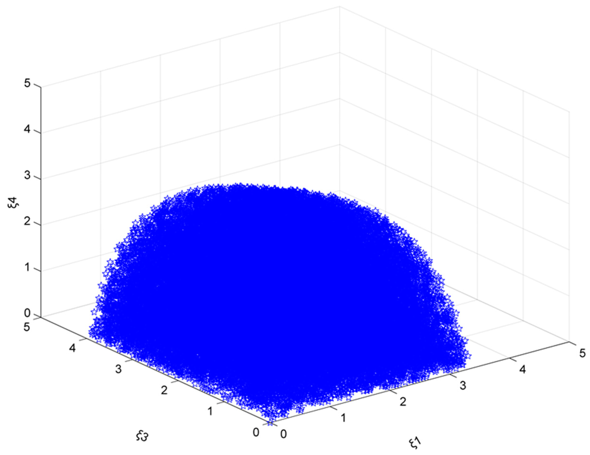
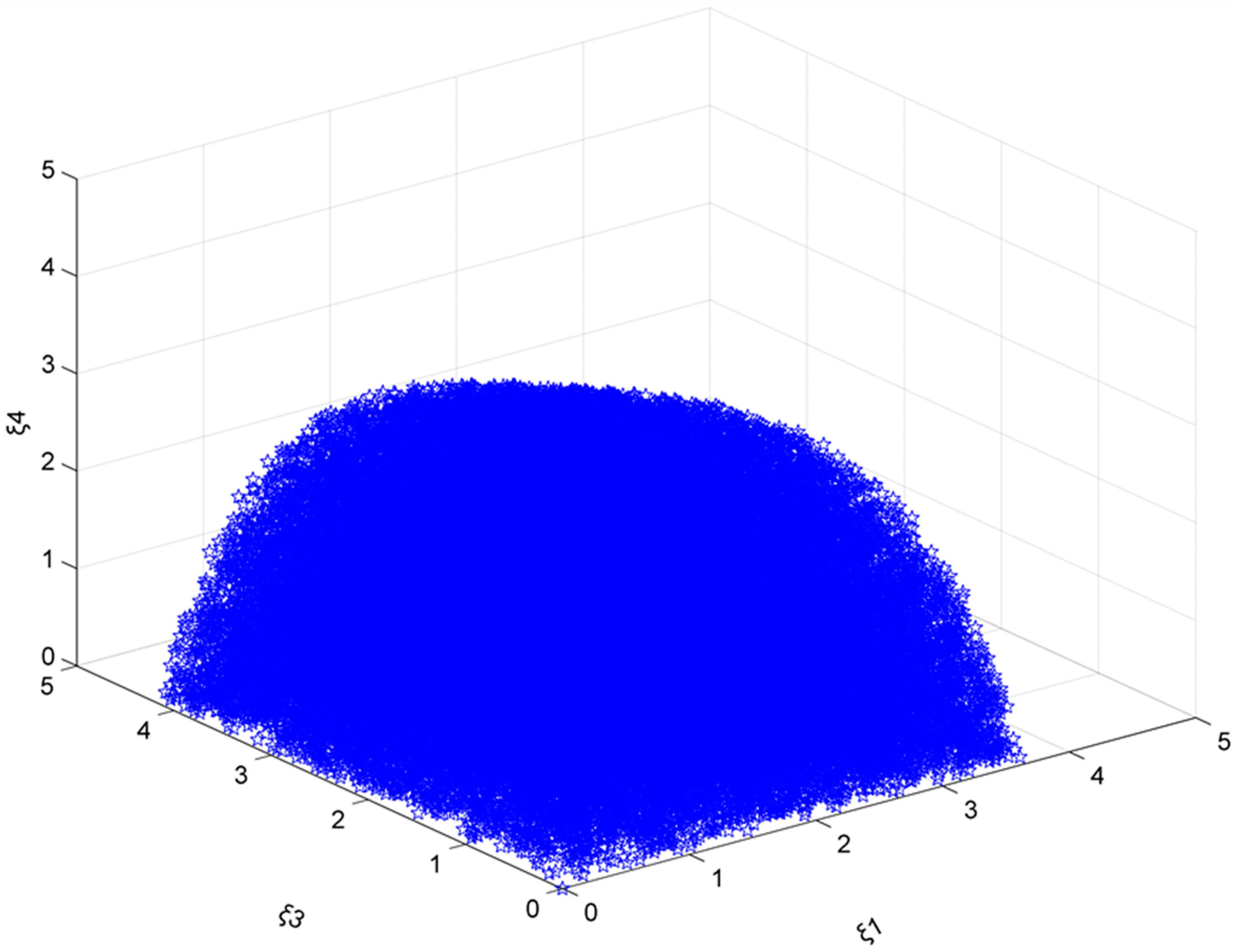
As the emission reduction target is 15%, ξ2, ξ5, and ξ6 are all set to 0 at the same time. The steel market stability domain composed of ξ1, ξ3, and ξ4 is analyzed. As can be seen in Figure 1, the adjustment coefficient ξ1 range is [0, 3.35], the ξ3 range is [0, 4.00], and the ξ4 range is [0, 5.00], (the ξ value range considered in this section is [0, 5], and the actual situation will not happen if the value is too large or negative, as can be seen below).

Figure 1.
The market stability domain (, with an emission reduction target of 15%).
Similarly, when the target increases from 16% to 20%, the steel market stability domain composed of ξ1, ξ3, and ξ4 is basically the same as when the target is 15%.
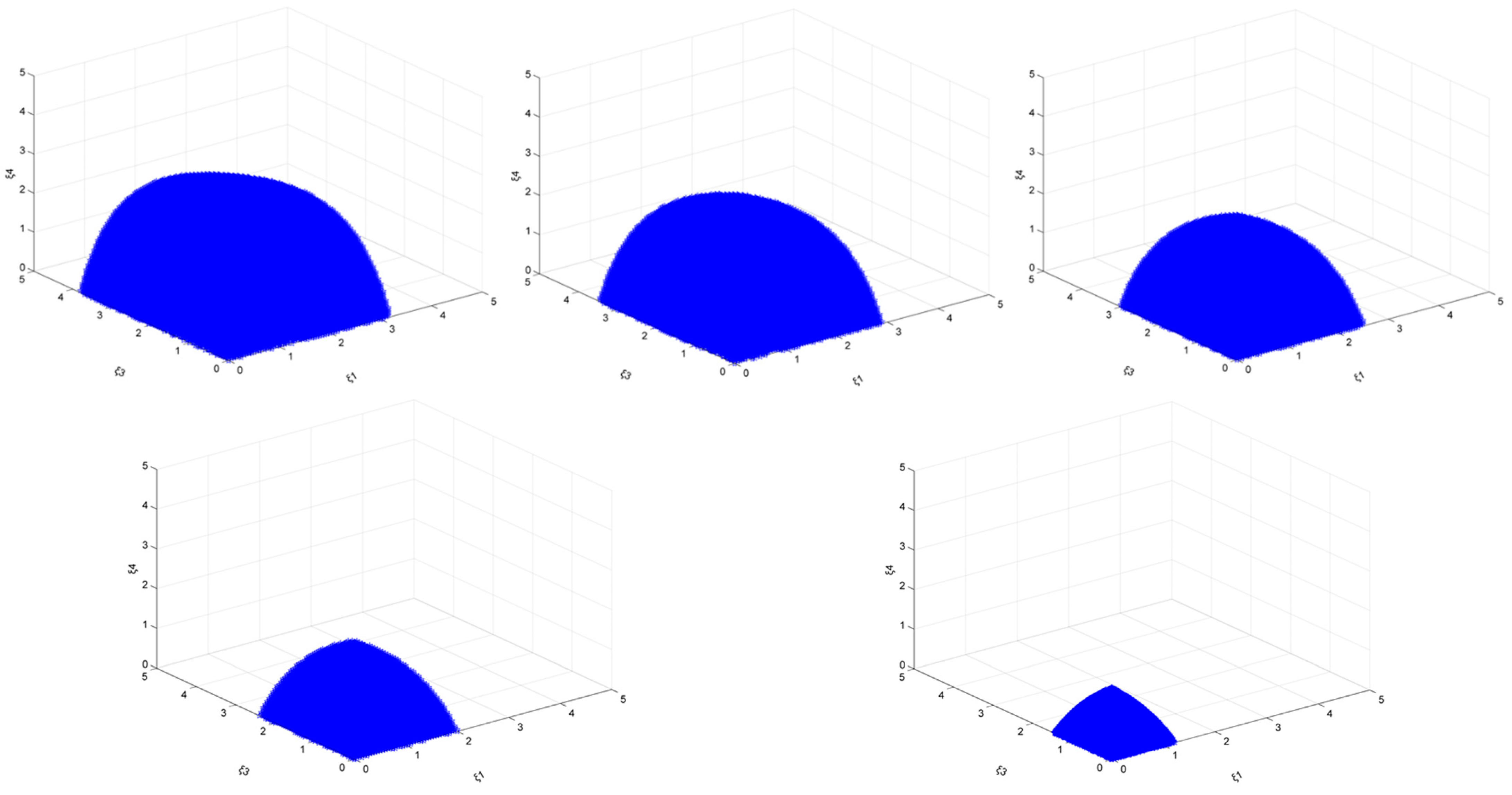
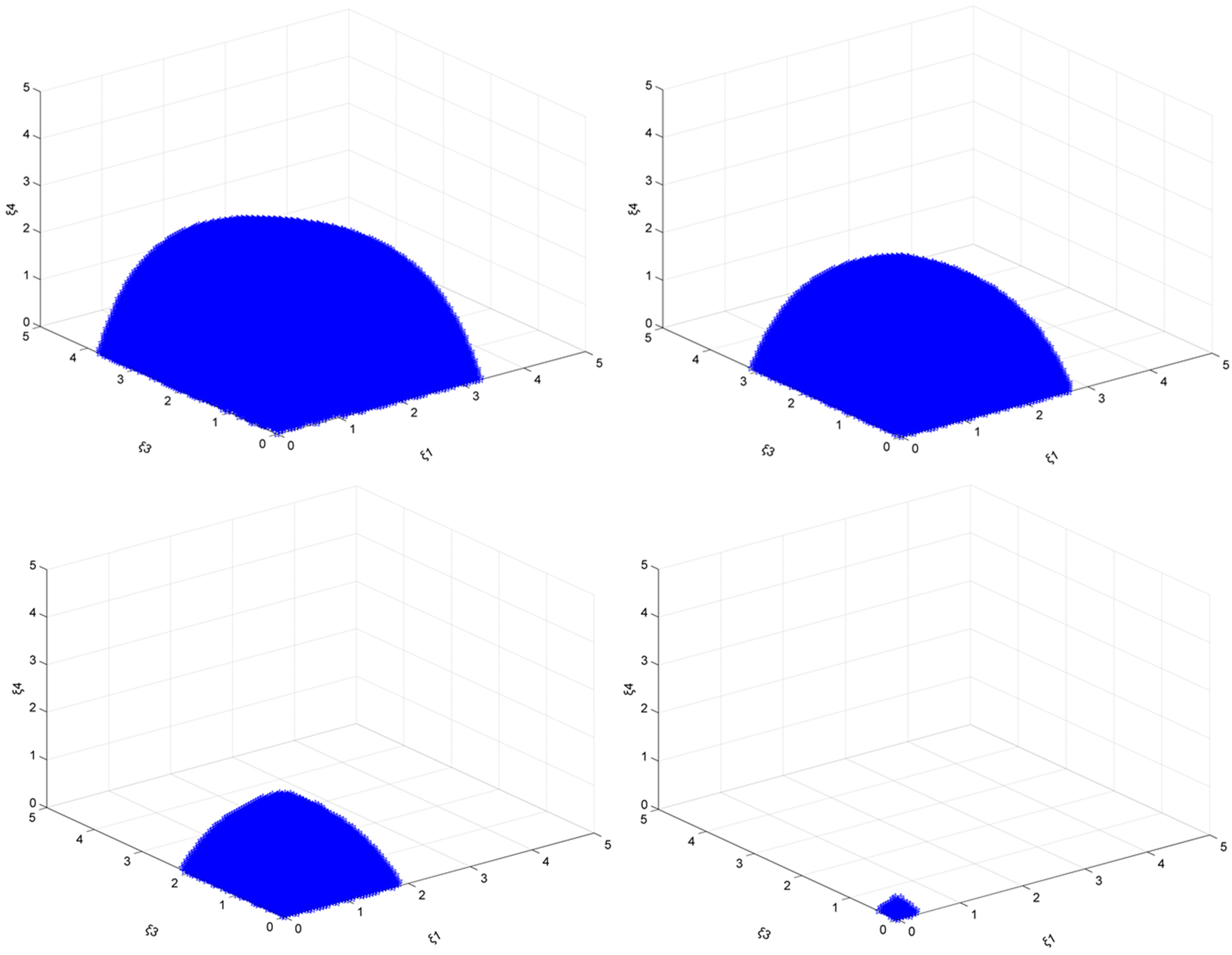
When the target is 15%, ξ2, ξ5, and ξ6 increase from 1.00 to 5.00 (Figure 2), and it can be seen that, as the northeast, southwest, and northwest regions adopt positive production adjustment coefficients at the same time, the stability of the steel market gradually decreases. When ξ2, ξ5, and ξ6 are large, the other three regions still have sufficient room for output adjustment.
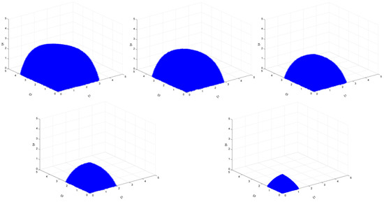
Figure 2.
The market stability domain (, with an emission reduction target of 15%).
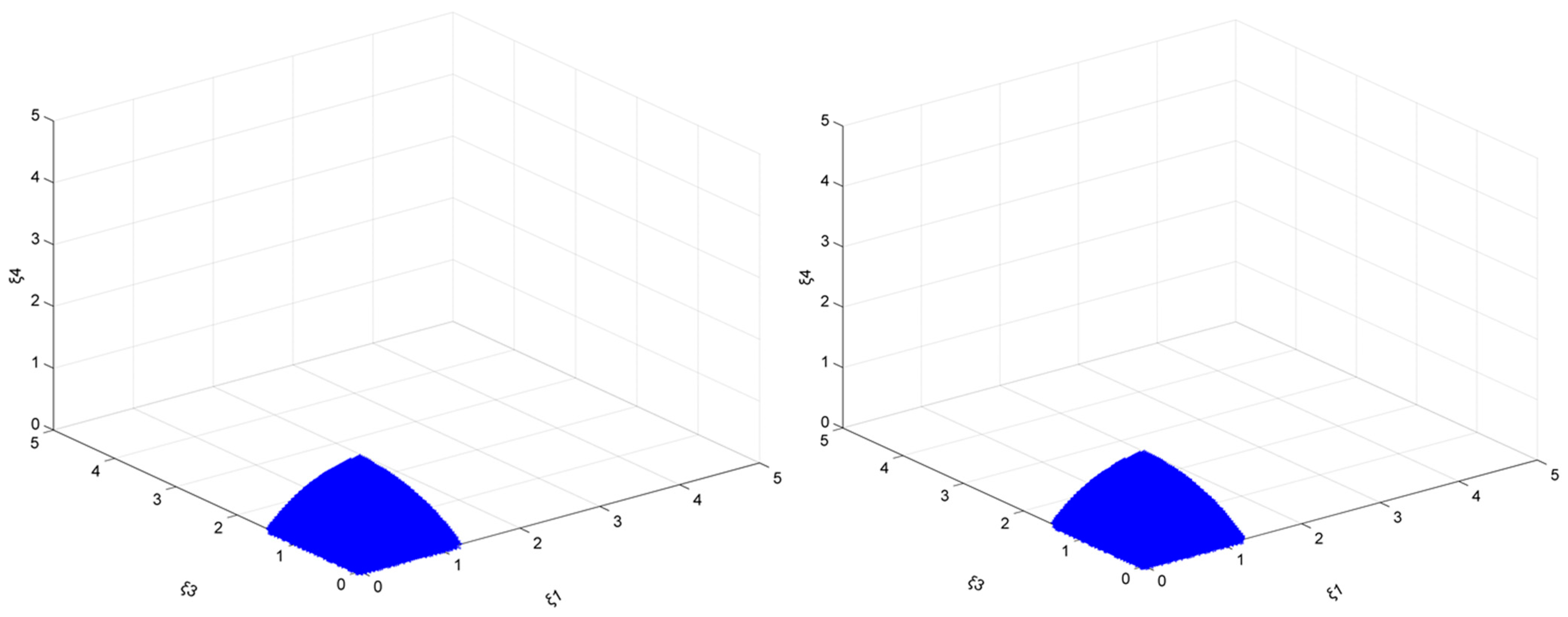
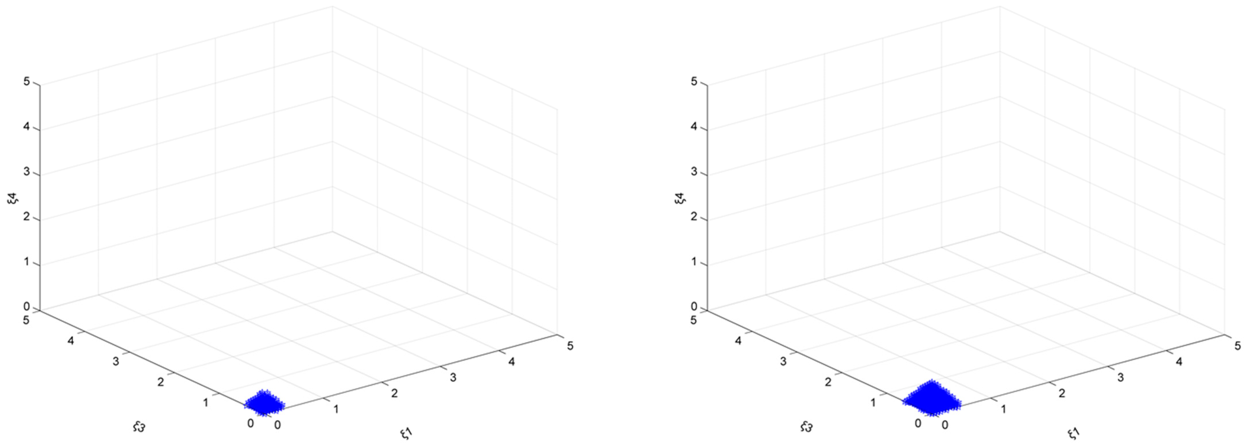
However, it should be pointed out that, when the target is small, the change in the stable region is almost unaffected. However, with the gradual increase in the target (take 20% as an example), the difference in the area of the stable region becomes more obvious. Take, as an example, the emission reduction targets of 15% and 20%, respectively, when ξ2, ξ5, and ξ6 are set to 5 at the same time. The results are shown in Figure 3:
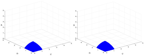
Figure 3.
The market stability domain (; the (left) emission target is 15%, while the (right) is 20%).
The value range of ξ1 remains at [0, 1.225], the value range of ξ3 is increased from [0, 1.450] to [0, 1.475], and the value range of ξ4 is increased from [0, 1.825] to [0, 1.850]. Judging from the results, the area of the stability region shows an increasing trend as the target increases. It shows that under the combined effect of the carbon tax and the output adjustment policy of smaller output enterprises, the larger output enterprises’ output adjustment policies will show an increasing trend.
- 2.
- The output adjustment speed of ξ1, ξ3, ξ4 remains unchanged.
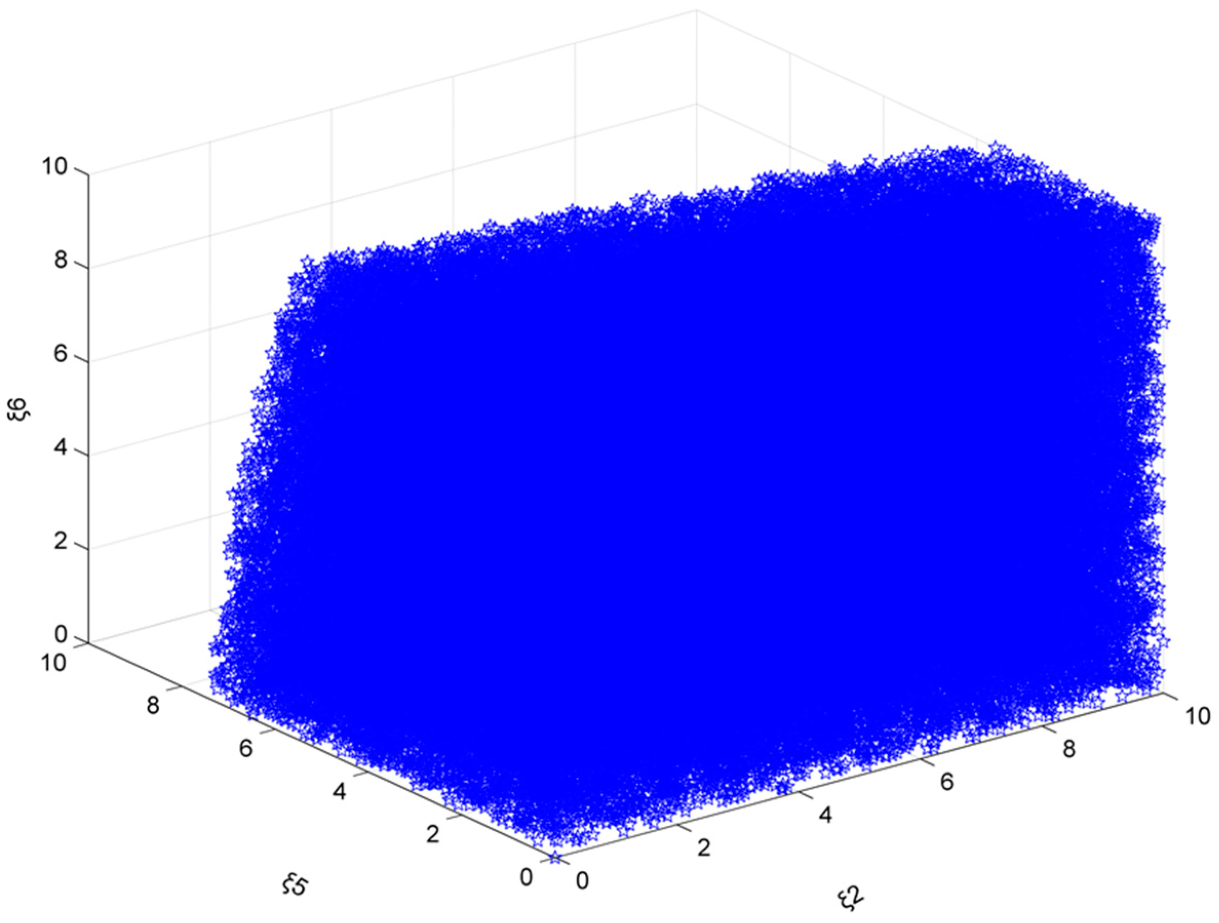
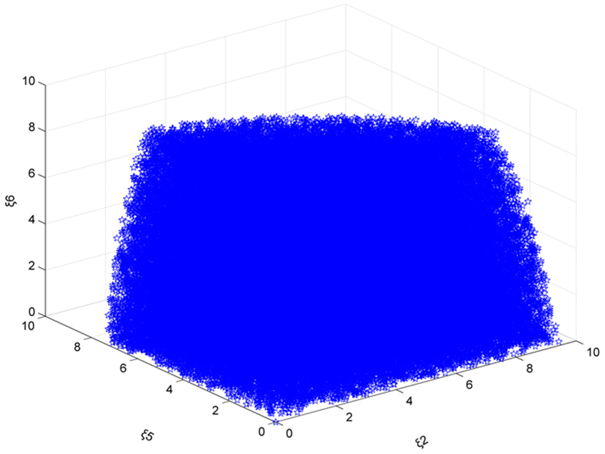
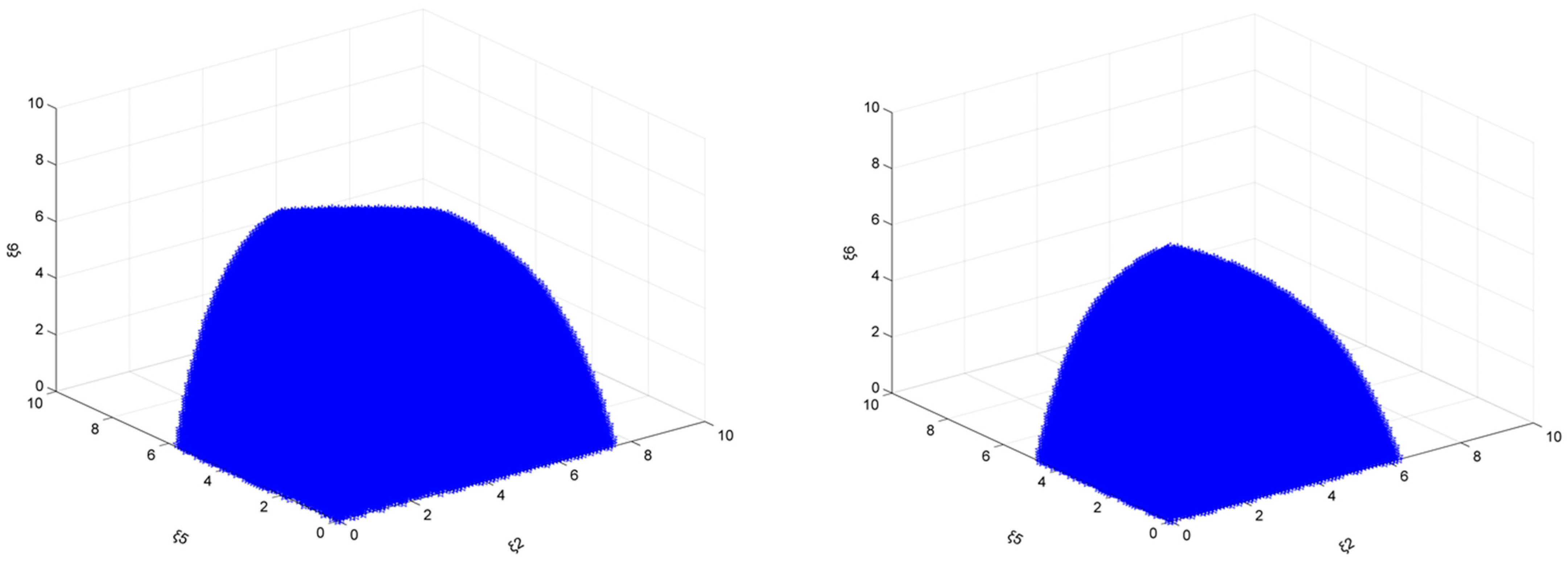
As the emission reduction target is 15%, and ξ1, ξ3, ξ4 are both set to 0, the steel market stability domain composed of ξ2, ξ5, and ξ6 is analyzed. As can be seen in Figure 4, the range of ξ2 is [0, 10.00], ξ5 is [0, 7.50], and ξ6 is [0, 10.00] or even more. The value range of ξ considered in this section is [0, 10].

Figure 4.
The market stability domain (, with an emission reduction target of 15%).
Similarly, when the target is gradually increased from 16% to 20%, the market stability domain composed of ξ2, ξ5, and ξ6 is basically the same as when the target is 15%.
When the target is 15%, ξ1, ξ3, and ξ4 simultaneously increase from 0.50 to 2.00. The stability domain is shown in Figure 5, where it can be seen that when North, East, and South Central China adopt positive production adjustment coefficients at the same time, the stability of the steel market gradually decreases. It can be clearly found that when ξ1, ξ3, and ξ4 take small positive values, Northeast China, Southwest China, and Northwest China still have greater autonomy in decision-making. However, when ξ1, ξ3, and ξ4 gradually increase, the stable area of the entire steel market will shrink sharply. When ξ1, ξ3, and ξ4 are 2, the value range of ξ2, ξ5, and ξ6 is very small. Obviously, when ξ1, ξ3, and ξ4 keep increasing, the market is easily out of balance.
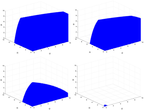
Figure 5.
The market stability domain (, with an emission reduction target of 15%).
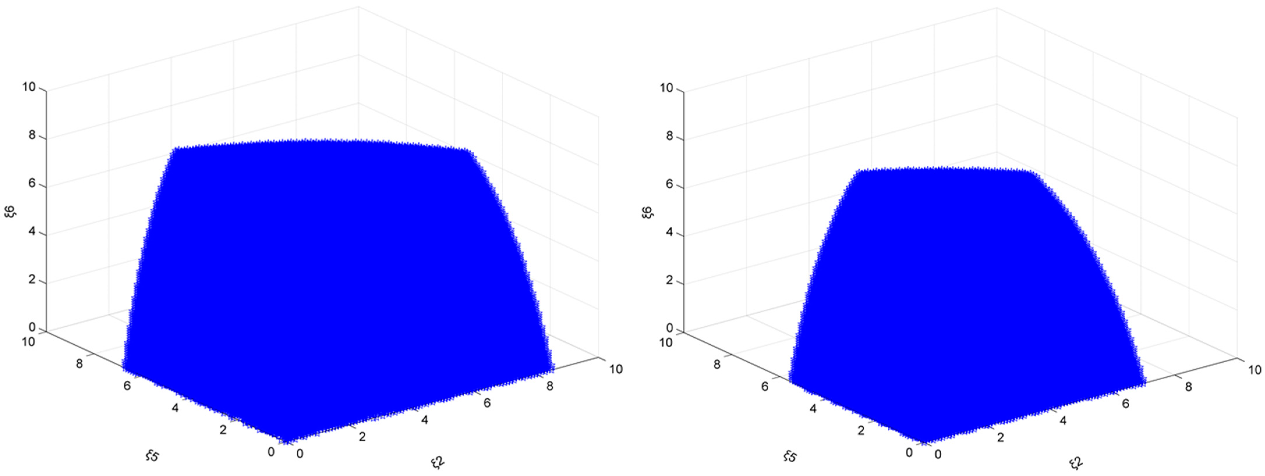
Similarly, although the shape and change trends of the stable region are very similar, and when the target is small (close to 15%), the change in the stable region is almost unchanged. However, when the target is high (take 20% as an example), the difference in the area of the stable region becomes more obvious. Take the emission reduction targets of 15% and 20%, respectively. When ξ1, ξ3, and ξ4 take 1.5 at the same time as an example, the results are shown in Figure 6.
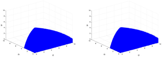
Figure 6.
The market stability domain (, and emission reduction targets of 15% on the (left), and 20% on the (right).
The value range of ξ2 is still maintained at [0, 10] (but through further calculations, the upper limit is increased), the value range of ξ5 is maintained at [0, 3.60], and the value range of ξ6 is increased from [0, 8.60] to [0, 8.80]. Judging from the results, the area of the stability region shows an increasing trend as the target increases. This means that, under the combined effect of the single carbon trading policy and the output adjustment policy of enterprises with larger output, the smaller output enterprises’ output adjustment policies will also increase.
- 3.
- System dynamic characteristics analysis.
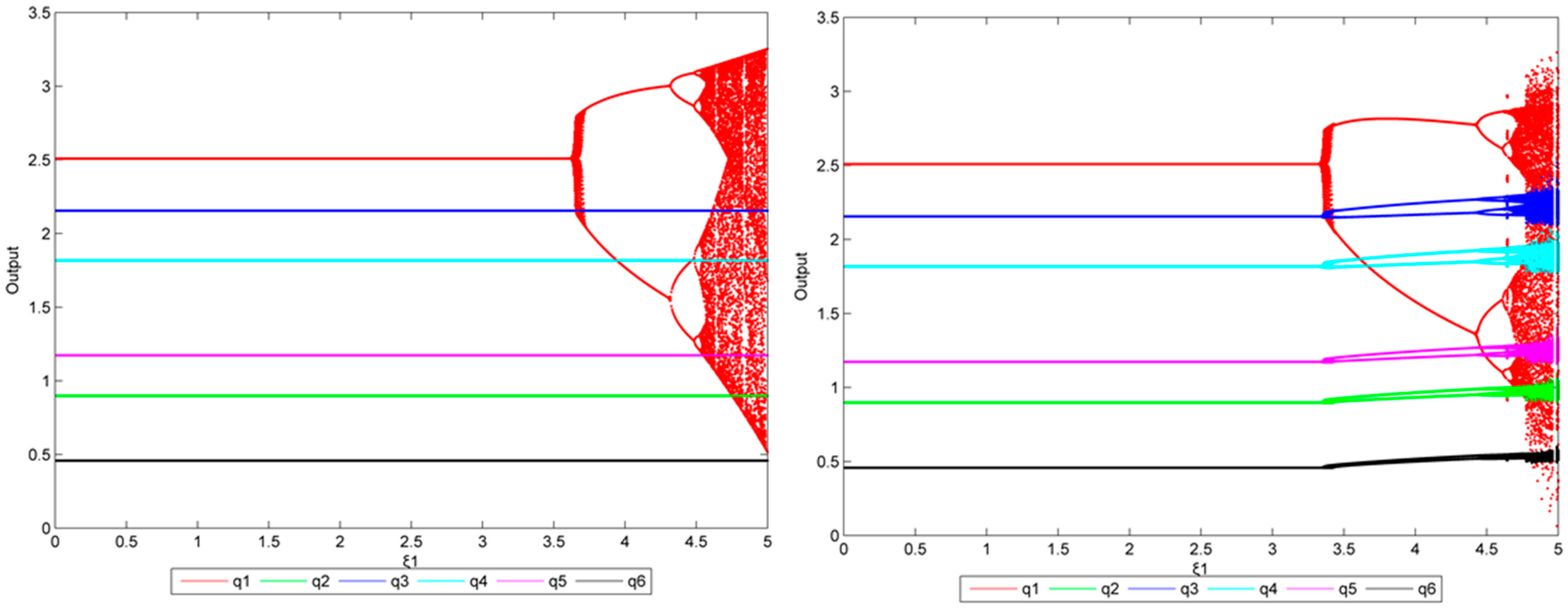
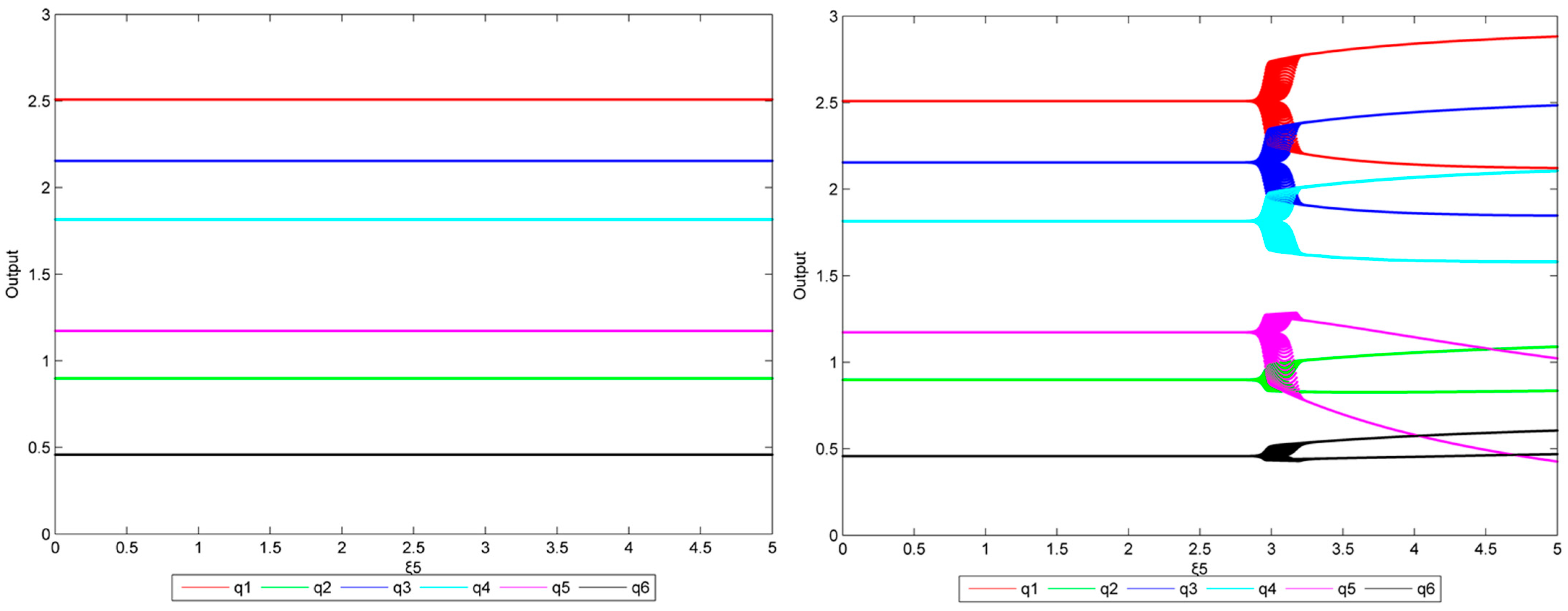
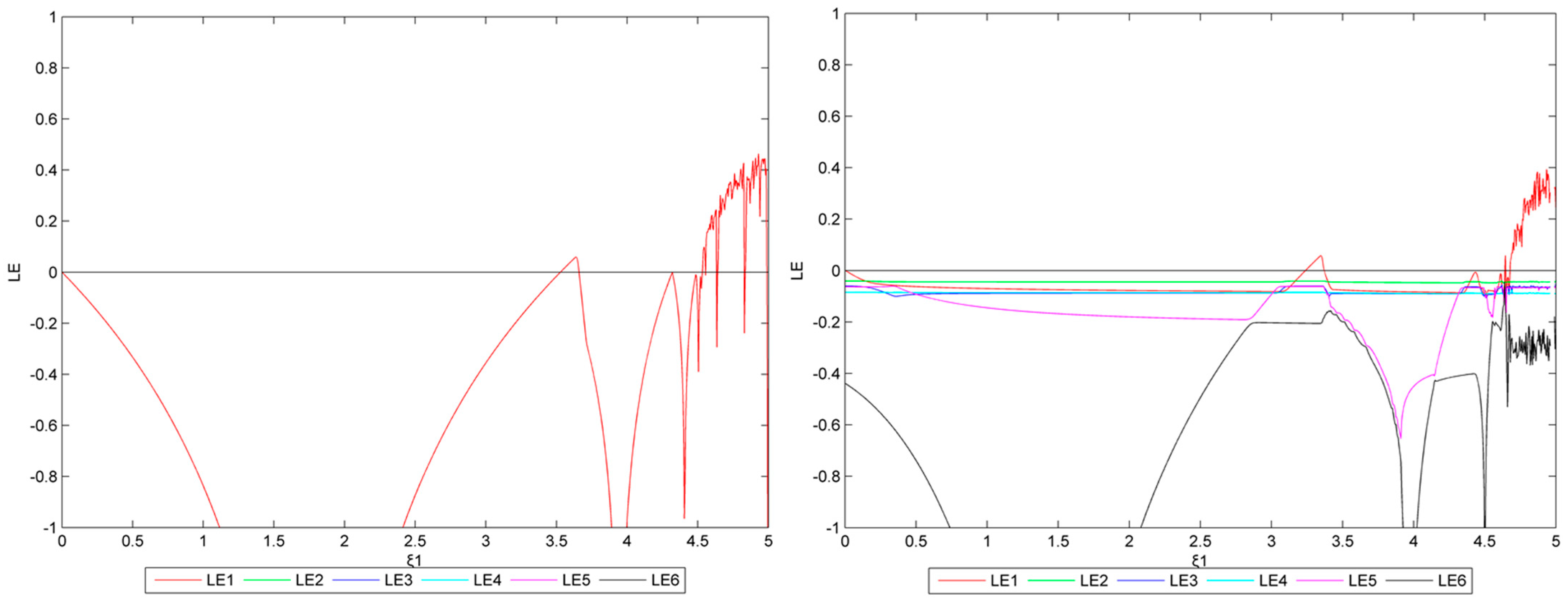
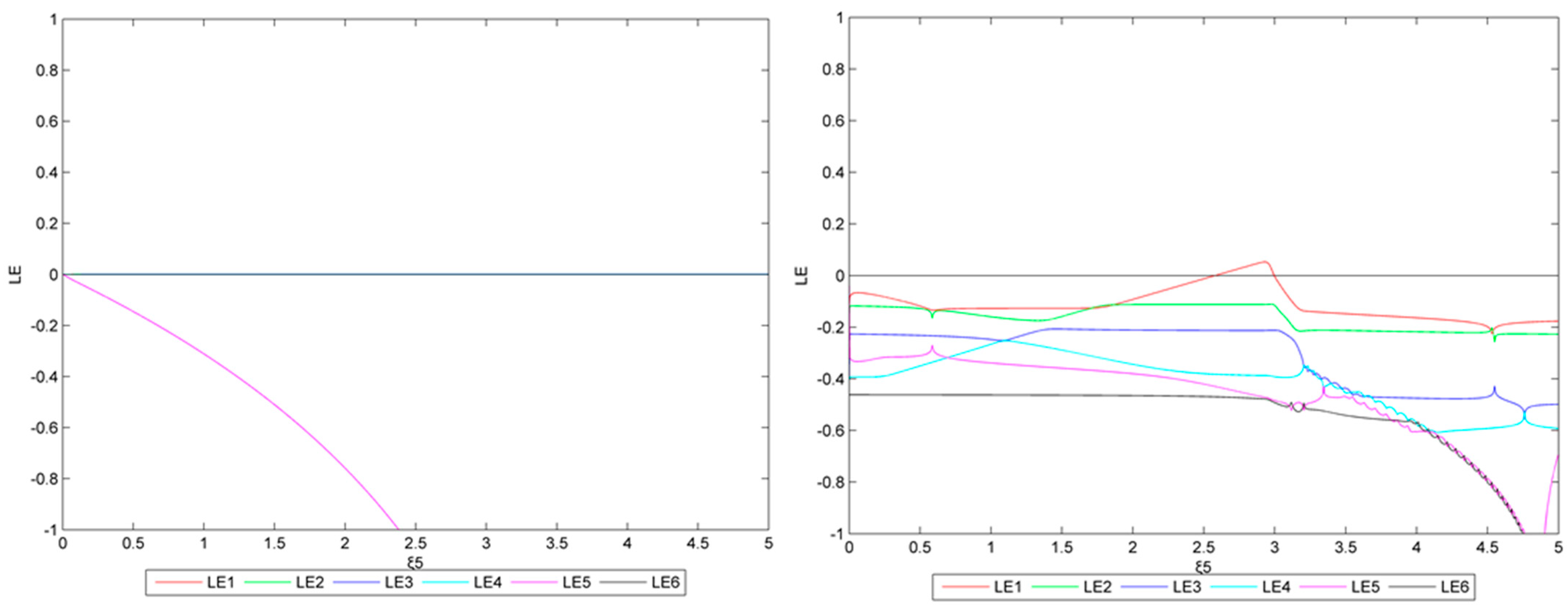
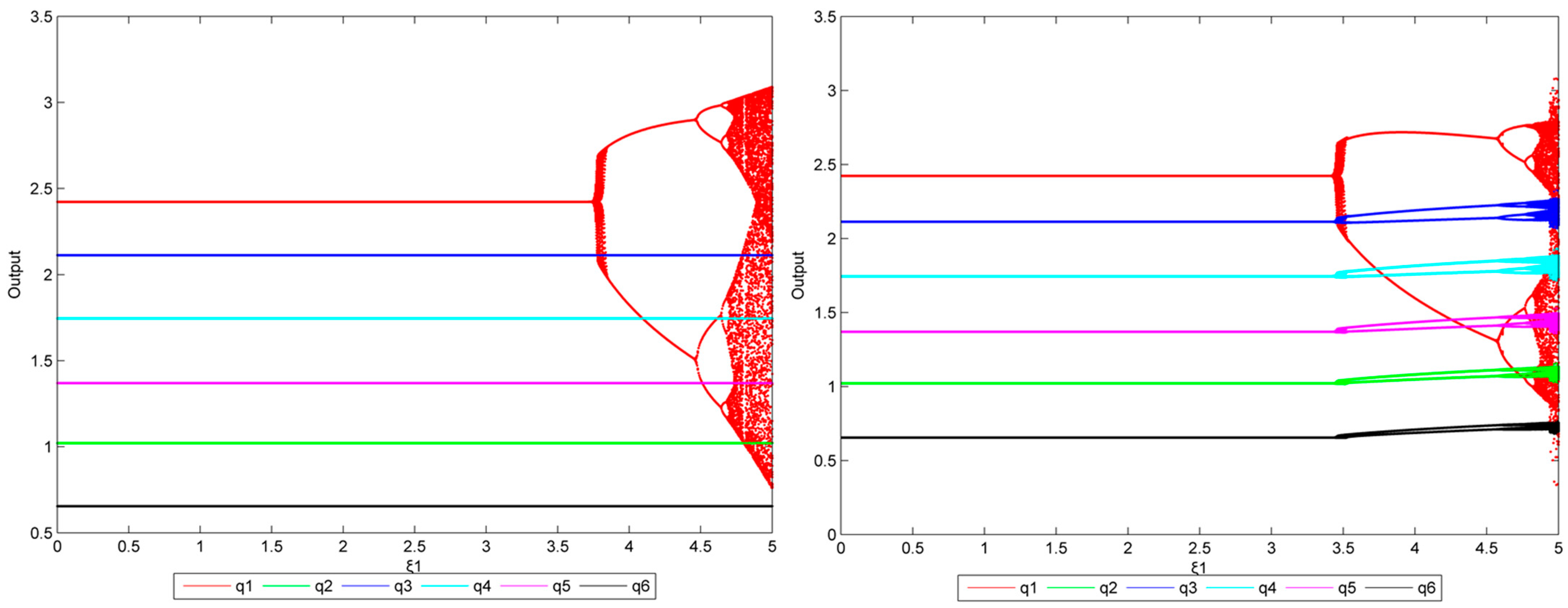
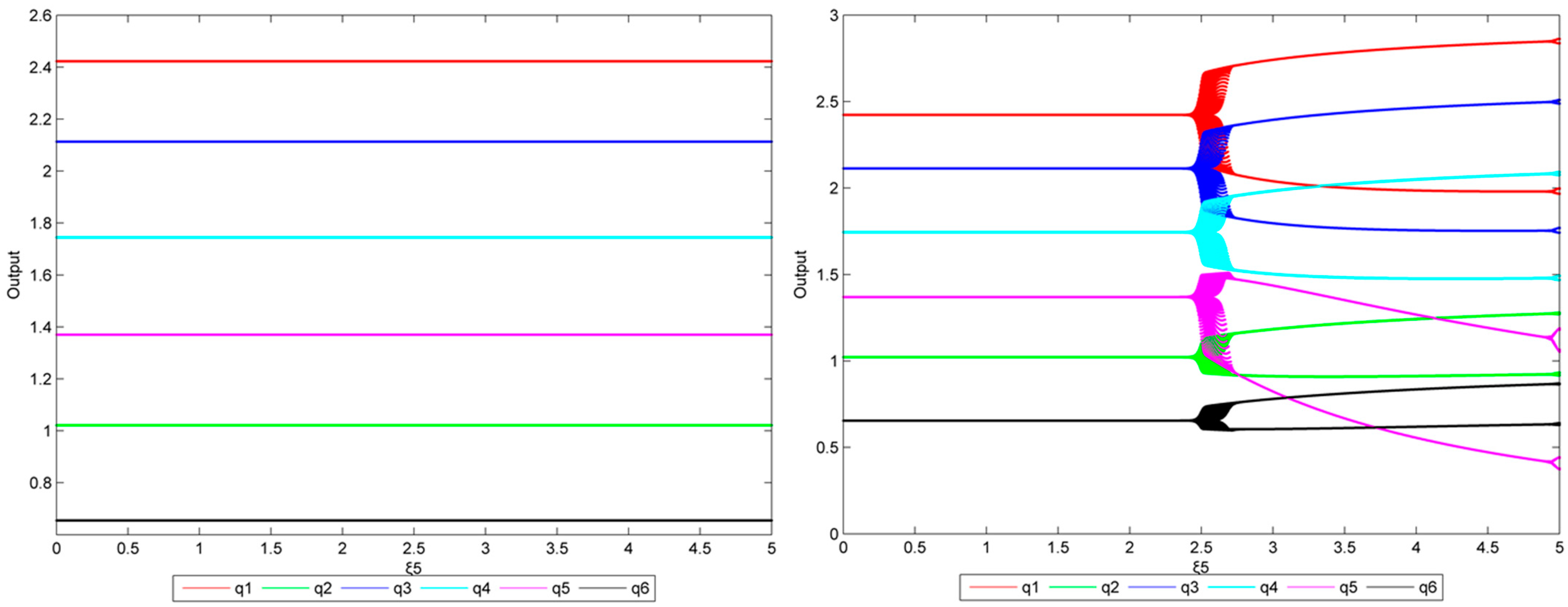
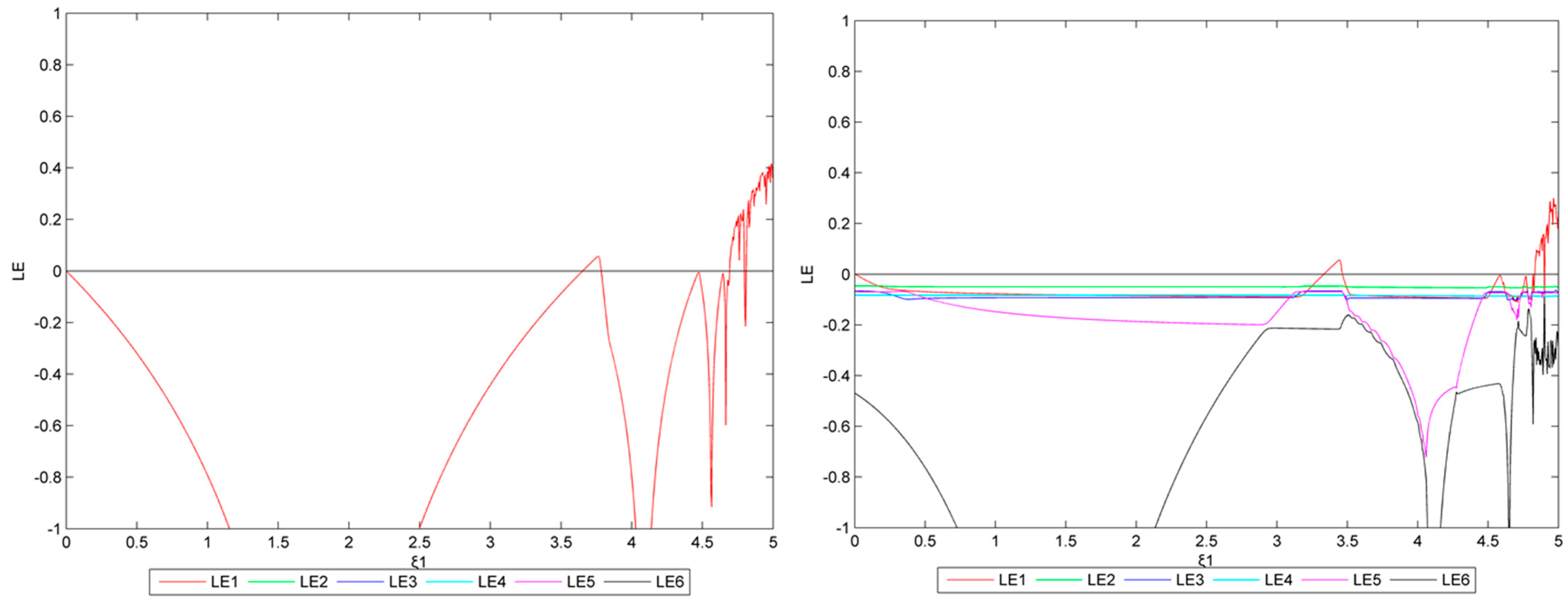
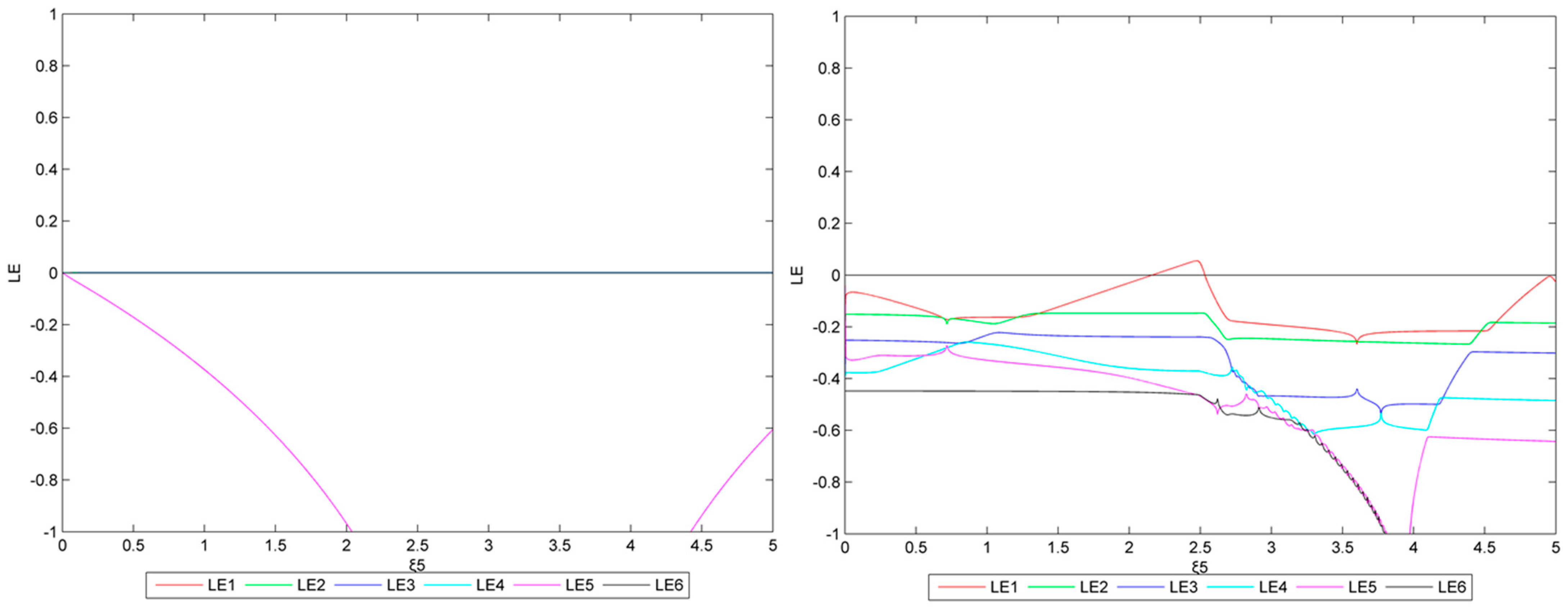
According to the previous research, this section selects two groups of representative enterprises, namely North China (representing larger output enterprises) and Southwest China (representing smaller output enterprises). Therefore, in this section, we will discuss ξ1, ξ5, and the change impacts on system stability (we actually calculated all the results with a reduction target of 15–20%, but due to space limitations, this section uses a reduction target of 20% as an example). The results are shown in Figure 7, Figure 8, Figure 9 and Figure 10.

Figure 7.
The bifurcation diagram of ((left): = 0, (right): = 0.4).

Figure 8.
The bifurcation diagram of ((left): = 0, (right): = 1.5).

Figure 9.
The Lyapunov exponent diagram ((left): = 0, (right): = 0.4).

Figure 10.
The Lyapunov exponent diagram ((left): = 0, (right): = 1.5).
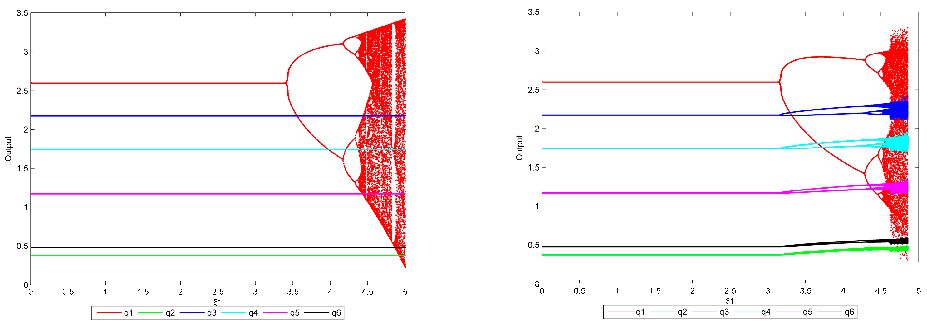
From the Figure 7, the following results can be obtained: when = 0 (left), the system is stable as is in the range of [0, 3.410]. Then, there is a small interval where is unstable. When the value increases to 3.420, the system is no longer balanced and it transitions from stable to double-cycle to chaos, but only North China has an output imbalance. When = 0.4 (right), the system is stable as is below 3.150. Then, there is a small interval, and in this interval production is unstable. When the value increases to 3.160, the system is no longer balanced and transitions from stable to double-cycle to chaos. However, the output of other regions appears unbalanced as gradually increases.
This shows that the system is more likely to fall into an unbalanced state when multiple enterprises use dynamic output adjustment at the same time instead of a single enterprise adopting output adjustment.
From Figure 8, when = 0 (left), the system remains in equilibrium regardless of . When are at 1.5 (right), the system is stable, as is below 3.015. Then, there is a small interval, and in this interval the production of all enterprises is unstable. When the value increases to 3.030, the system is no longer balanced and transitions from stable to double-cycle to chaos.
From the results of Figure 7 and Figure 8, the larger output enterprises can have a much greater impact on the system balance than those smaller output enterprises, and misadjusted adjustment of output by these larger producers will easily create market imbalance. With the gradually increasing emission reduction targets, the enterprises’ policies of output adjustment could be more flexible and diverse, and the system will be in a state of bifurcation and chaos.
Figure 9 and Figure 10 show the Lyapunov exponents for Figure 7 and Figure 8. When = 0 and = 3.420 (left in Figure 9), the system shows bifurcation. When > 4.365, the maximum Lyapunov exponent changes from negative to positive, and the system is in chaos. When are 0.4 and = 3.160 (right in Figure 9), bifurcation appears and then all enterprises bifurcate. When > 4.490, the maximum Lyapunov exponent changes from negative to positive, and the system becomes chaotic.
When are 0 (left in Figure 10), the maximum Lyapunov exponent is always negative. When equal 1.5 (right in Figure 10) and ranges from 3.005 to 3.015, the maximum Lyapunov exponent changes from negative to positive, and there are bifurcations in various regions. When > 3.015, the maximum Lyapunov exponent is no longer positive, while the system becomes a double-cycle.
4.2.2. Mixed Carbon Trading Policy Scenario in 2025: Carbon Trading + Subsidy
In this scenario, the equilibrium output E* of each regional enterprise with different emission reduction targets are are shown in Table 7 and Table 8.

Table 7.
The equilibrium output E* of each regional enterprise (emission reduction target of 20–25%, e0 = 2.3782).

Table 8.
The equilibrium output E* of each regional enterprise (emission reduction target of 20–25%, e0 = 2.2197).
And the Jacobian matrix J obtained are as shown in Table 9 (e0 = 2.3782) and Table 10 (e0 = 2.2197).

Table 9.
The Jacobian matrix J (emission reduction target of 20–25%, e0 = 2.3782).

Table 10.
The Jacobian matrix J (emission reduction target of 20–25%, e0 = 2.2197).
In order to facilitate discussion and save space, this section only discusses the relevant calculation results under the scenarios of 20% and 25% emission reductions.
- 4.
- The output adjustment speed of ξ2, ξ5, ξ6 remains unchanged.
As e0 = 2.3782, emission reduction target is 20%, and ξ2, ξ5, and ξ6 take 0 at the same time, the steel market stability domain composed of ξ1, ξ3, and ξ4 is analyzed. As can be seen in Figure 11, the adjustment coefficient ξ1 range is [0, 3.50], the ξ3 range is [0, 4.05], and the ξ4 range is [0, 4.75].
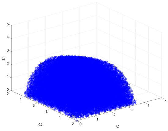
Figure 11.
The market stability domain (, with an emission reduction target of 20%, e0 = 2.3782).
As the target is 20%, ξ2, ξ5, and ξ6 change from 1.00 to 4.00 (Figure 12), and the stable area gradually decreases. The changing trend of its shape is very similar to that of a single carbon trading policy. However, the difference is that when the values of ξ2, ξ5, and ξ6 are large (=4), the area of its stability region has been greatly reduced, but when ξ2, ξ5, and ξ6 continue to increase to 5, there is no region left. This shows that with the introduction of the mixed emission reduction policy, the output adjustment policy of enterprises has been compressed, and enterprises with larger output have to carefully consider their next production strategy to prevent the entire steel market from falling into an imbalance.


Figure 12.
The market stability domain (, with an emission reduction target of 20%).
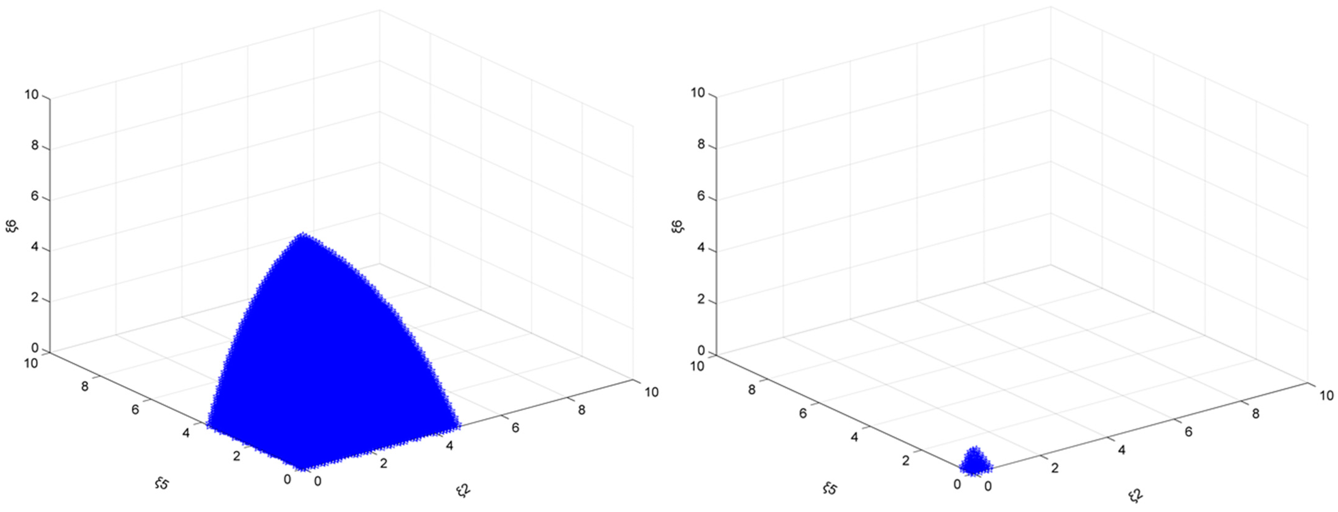
When the targets gradually increase, the change trends in the market stable region are basically similar, and these also decrease rapidly with the increase in . However, when , the stable regions of Northeast, Southwest, and Northwest China increase. Additionally, when the targets gradually increase, the stable region shows an increasing trend (of course, the increased area is still small). Take the emission reduction targets of 20% and 25% respectively, when ξ2, ξ5, and ξ6 are set to 5 at the same time as an example. This is shown in Figure 13.

Figure 13.
The market stability domain (, with an emission reduction target of 20% on the (left), and 25% on the (right)).
When the target increases from 20% to 25%, the stability domain, which was nonexistent, became significantly larger. The value range of ξ1 is expanded to [0, 0.075], the value range of ξ3 is expanded to [0, 0.100], and the value range of ξ4 is expanded to [0, 0.125]. This shows that under a mixed emission reduction policy, under the combined effect of the emission reduction policy and the output adjustment policy of an enterprise with a smaller output, as the target gradually increases, the output adjustment policies of enterprises with larger outputs will show an increasing trend.
When e0 gradually decreases, that is, the benchmark value in the carbon trading mechanism becomes more and more stringent, in fact, the change rule of the stable region does not change much, except for the difference in area. Take e0 = 2.3782, 2.3148 and 2.2197, , and the emission reduction target of 25% as an example. Here, remains in the range of [0, 0.075], remains in the range of [0, 0.100], while reduces from [0, 0.125] to [0, 0.100]. It can be foreseen that, when the benchmark value is lower, the stable region may cease to exist.
- 5.
- The output adjustment speed of ξ1, ξ3, ξ4 remains unchanged.
As e0 = 2.3782, the target is 20%, and ξ1, ξ3, and ξ4 are taken as 0 at the same time, the steel market stability domain composed of ξ2, ξ5, and ξ6 is analyzed. As can be seen in Figure 14, the adjustment coefficient ξ2 range is [0, 9.50], the ξ5 range is [0, 7.40], and the ξ6 range is [0, 10.00] or even more.
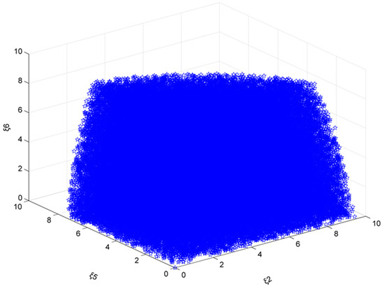
Figure 14.
The market stability domain (, with an emission reduction target of 20%).
Figure 15 shows that when the target is 20%, the steel market stability domain (ξ1, ξ3, ξ4) increases from 0.50 to 2.00.

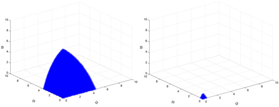
Figure 15.
The market stability domain (, with an emission reduction target of 20%).
From the results, the stability domain is gradually decreasing, but the difference is that the decrease in the area of the stability region under this scenario is even more dramatic. For example, when ξ1, ξ3, and ξ4 are 1.5, the output adjustment space of the other three regions is as follows: ξ2 is [0, 4.70], ξ5 is [0, 3.70], ξ6 is [0, 9.20]; compared to only a single carbon trading policy scenario (when the target is 20%), its stability area has been greatly reduced. When the values of ξ1, ξ3, and ξ4 are larger, it is foreseeable that the moment of system imbalance will be earlier than the situation where there is only a single carbon trading policy scenario (when the target is 20%).
Similarly, when the target is increased from 20% to 25%, and when ξ1, ξ3, and ξ4 take 1.5 at the same time, the value range of ξ2 is maintained at [0, 4.70], the value range of ξ5 is maintained at [0, 3.70], and the value range of ξ6 is increased from [0, 9.20] to [0, 9.30]. When ξ1, ξ3, and ξ4 take other smaller values, there is a similar rule. However, when ξ1, ξ3, and ξ4 assume larger values at the same time (and there is a stable region), the conclusion is different. When the target is increased from 20% to 25%, ξ1, ξ3, and ξ4 are 2, the value range of ξ6 maintained in the interval of [0, 0.90], but the value range of ξ2 is reduced from [0, 0.50] to [0, 0.40], and the value range of ξ2 is reduced from [0, 0.40] to [0, 0.30]. These results are shown in Figure 16 and Figure 17.

Figure 16.
The market stability domain (, for the emission reduction target of 20% in 2020 on the (left), 20% in 2025 in the (middle), and 25% on the (right)).

Figure 17.
The market stability domain (, with an emission reduction target if 20% in 2020 on the (left) 20%, 20% in 2025 in the (middle), and 25% on the (right)).
When e0 gradually decreases, that is, the benchmark value in the carbon trading mechanism becomes more and more stringent; in fact, the change rule of the stable region does not change much, except for the difference in area. Take e0 = 2.3782, 2.3148 and 2.2197, and the emission reduction target of 25% as an example. Here, remains in the range of [0, 9.700], remains in the range of [0, 10.000], while reduces from [0, 7.500] to [0, 7.400]. The changes in are so small that they were almost negligible. Unless e0 is very small, the change is obvious, but that is too extreme.
This illustrates that when the government adopts a mix of emission reduction policies, under the combined effect of these policies and output adjustment policy of the larger output enterprise, the smaller output enterprise adjustment policy will be restricted or affected by more factors. The rule of change is different from that of a single carbon trading scenario, and the change rule of the stable region is very uncertain, which is related to the enterprise’s own output, emission reduction target, carbon trading benchmark value, etc. This means that enterprises with a smaller output need to be more cautious in formulating their own production plans to ensure that the enterprises and the entire steel market will not fall into an imbalanced state.
- 6.
- System dynamic characteristics analysis.
In this part, we have actually calculated all the results with a reduction target of 20–25% but, due to space limitations, this part uses a reduction target of 25% (e0 = 2.3782) as an example for discussion.
From the Figure 18, the following results can be obtained: when = 0 (left), the system is stable as is in the range of [0, 3.625]. Then, there is a small interval where is unstable. When the value increases to 3.630, the system is no longer balanced and transitions from stable to double-cycle to chaos, but only North China has an output imbalance. When = 0.4 (right), the system is stable as is below 3.335. Then, there is a small interval, and in this interval production is unstable. When the value increases to 3.340, the system is no longer balanced and transitions from stable to double-cycle to chaos. However, the output of other regions appears unbalanced as gradually increases.
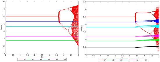
Figure 18.
The bifurcation diagram of ((left): = 0, (right): = 0.4).
From Figure 19, when = 0 (left), the system remains in equilibrium regardless of . When are at 1.5 (right), the system is stable, as is below 2.890. Then, there is a small interval, and in this interval the production of all enterprises is unstable. When the value increases to 2.930, the system is no longer balanced and transitions from stable to double-cycle to chaos.
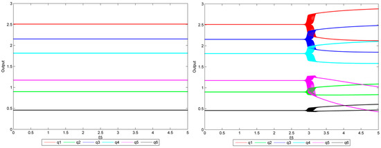
Figure 19.
The bifurcation diagram of ((left): = 0, (right): = 1.5).
Figure 20 and Figure 21 show the Lyapunov exponents for Figure 18 and Figure 19. When = 0 and = 3.625 (left in Figure 20), the system shows bifurcation. When > 4.520, the maximum Lyapunov exponent changes from negative to positive, and the system is in chaos. When are 0.4 and = 3.335 (right in Figure 20), bifurcation appears and then all enterprises bifurcate. When > 4.645, the maximum Lyapunov exponent changes from negative to positive, and the system becomes chaotic.
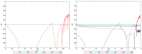
Figure 20.
The Lyapunov exponent diagram ((left): = 0, (right): = 0.4).
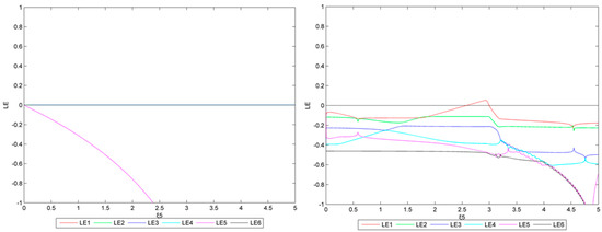
Figure 21.
The Lyapunov exponent diagram ((left): = 0, (right): = 1.5).
When are 0 (left in Figure 21), the maximum Lyapunov exponent is always negative. When equal 1.5 (right in Figure 21) and range from 2.580 to 2.930, the maximum Lyapunov exponent changes from negative to positive, and there are bifurcations in various regions. When > 2.930, the maximum Lyapunov exponent is no longer positive, while the system becomes a double-cycle.
4.2.3. Multiple Mixed Carbon Trading Policy Implemented in 2030: Carbon Trading + Subsidy + CCS
In this scenario, the equilibrium output E* of each regional enterprise with different emission reduction targets are as shown in in Table 11 and Table 12.

Table 11.
The equilibrium output E* of each regional enterprise (emission reduction target: 25–30%, e0 = 2.2197).

Table 12.
The equilibrium output E* of each regional enterprise (emission reduction target of 25–30%, e0 = 2.0611).
And the Jacobian matrix J obtained are as shown in Table 13 (e0 = 2.2197) and Table 14 (e0 = 2.0611).

Table 13.
The Jacobian matrix J (emission reduction target of 25–30%, e0 = 2.2197).

Table 14.
The Jacobian matrix J (emission reduction target of 25–30%, e0 = 2.0611).
In order to facilitate discussion and save space, this part only discusses the relevant calculation results under the scenarios of 25% and 30% emission reductions.
- 7.
- The output adjustment speed of ξ2, ξ5, ξ6 remains unchanged.
As e0 = 2.2197, the target is 25%, and ξ2, ξ5, and ξ6 take 0 at the same time, the steel market stability region consisting of ξ1, ξ3, and ξ4 is analyzed. As can be seen in Figure 22, the adjustment coefficient ξ1 range is [0, 3.65], the ξ3 range is [0, 4.15], and theξ4 range is [0, 5.00].

Figure 22.
The market stability domain (, emission reduction target: 25%).
As the target is 25%, ξ2, ξ5, and ξ6 change from 1.00 to 4.00 (Figure 23), and the stable area gradually decreases. However, the difference is that when the values of ξ2, ξ5, and ξ6 are large (=4), compared to the mixed carbon trading policy scenario (emission reduction target = 25%), the area of its stability region has been greatly reduced. When ξ2, ξ5, and ξ6 continue to increase to 5, there is no longer a stable region. This shows that with the introduction of the multiple emission reduction policies, enterprises with larger output have to carefully consider their future production strategies to avoid output adjustment strategies that would spur the entire steel market into an imbalance.

Figure 23.
The market stability domain (, with an emission reduction target of 25%).
On the other hand, when the targets gradually increase, the stability region also shows a certain tendency to become larger. Take the emission reduction targets of 25% and 30% respectively, when ξ2, ξ5, and ξ6 are taken as 4 at the same time as an example. This is shown in Figure 24.
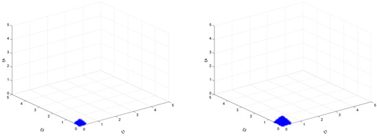
Figure 24.
The market stability domain (, with an emission reduction target of 25% on the (left) 25%, and 30% on the (right)).
When the target increases from 25% to 30%, the value range of ξ1 is increased from [0, 0.30] to [0, 0.45], the value range of ξ3 is increased from [0, 0.40] to [0, 0.60], and the value range of ξ4 is increased from [0, 0.45] to [0, 0.70]. This also shows that even if there are more complex mixed emission reduction policies, under the combined effect of emission reduction policies and output adjustment policies for enterprises with smaller output, as the target gradually increases, the output adjustment policies that affect enterprises with a larger output will show an increasing trend.
When e0 gradually decreases, that is, the benchmark value in the carbon trading mechanism becomes more and more stringent, the change rule of the stable region does not change much, except for the difference in area. Take e0 = 2.2197, 2.1563, and 2.0611, , and an emission reduction target of 30% as an example. Here, reduces from [0, 0.450] to [0, 0.400], reduces from [0, 0.600] to [0, 0.500], while reduces from [0, 0.700] to [0, 0.600]. It can be foreseen that when the benchmark value is lower, the stable region may cease to exist.
- 8.
- The output adjustment speed of ξ1, ξ3, ξ4 remains unchanged.
When e0 = 2.2197, the emission reduction target is 25%, and ξ1, ξ3, and ξ4 are taken as 0 at the same time, the steel market stability domain composed of ξ2, ξ5, and ξ6 is analyzed. As can be seen in Figure 25, the adjustment coefficient ξ2 range is [0, 8.30], the ξ5 range is [0, 6.30], and the ξ6 range is [0, 10.00] or even more, which is smaller than the scenario of a carbon trading and subsidy policy with a target of 25%. This shows that when the policies become more complex, the production plans of enterprises with smaller output will be affected more obviously.
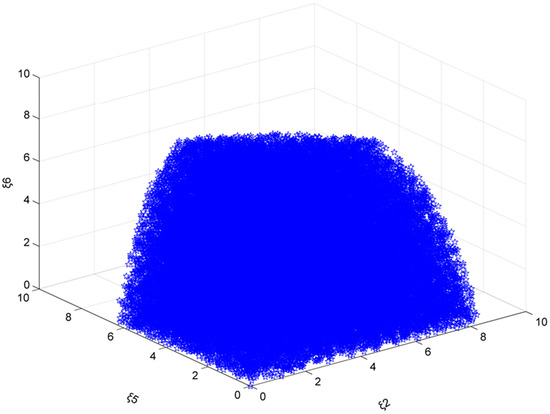
Figure 25.
The market stability domain (, with an emission reduction target of 25%).
Figure 26 shows that when the target is 25%, the steel market stability domain (ξ1, ξ3, ξ4) increases from 0.50 to 2.00.

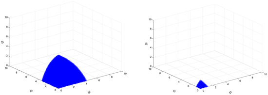
Figure 26.
The market stability domain (, with an emission reduction target of 25%).
From the results, the overall stability domain shows a gradual decrease trend, but compared with the previous model, the conclusion is slightly different. For example, when ξ1, ξ3, and ξ4 are 1.5, the output adjustment space of the other three regions is as follows: ξ2 is [0, 4.40], ξ5 is [0, 3.30], and ξ6 is [0, 6.80]. Compared to the scenario of carbon trading and a subsidy (an emission reduction target of 25%, where ξ2 is [0, 4.70], ξ5 is [0, 3.60], and ξ6 is [0, 9.30]), the area of its stability area has been greatly reduced. However, when the value of ξ1, ξ3, and ξ4 is larger (=2), the area of the stability region is bigger than the results of the mixed policy scenario (carbon trading and a subsidy, with a target of 25%). When ξ1, ξ3, and ξ4 continue to increase, the system will enter a state of imbalance, but the moment of system imbalance will be later than in the carbon trading and subsidy emission reduction policy scenario (the target is 25%).
Similarly, when the target is increased from 25% to 30%, and ξ1, ξ3, and ξ4 are 1.5 at the same time, the value range of ξ6 is increased from [0, 6.80] to [0, 6.90], the value range of ξ2 is maintained at [0, 4.40], and the value range of ξ5 is maintained at [0, 3.30]. When ξ1, ξ3, ξ4 are other smaller values, there is a similar rule. However, when ξ1, ξ3, and ξ4 take on larger values at the same time (and there is a stable region), the conclusion is different. When the target is increased from 25% to 30%, and when ξ1, ξ3, and ξ4 are given the value of 2 at the same time, the value range of ξ2 is reduced from [0, 1.10] to [0, 1.00], the value range of ξ5 is reduced from [0, 0.80] to [0, 0.70], and the value range of ξ6 is reduced from [0, 1.70] to [0, 1.40]. These results are shown in Figure 27 and Figure 28.

Figure 27.
The market stability domain (, with an emission reduction target of 25% in 2025 on the (left), 25% in 2030 in the (middle) 25%, and 30% on the (right)).

Figure 28.
The market stability domain (, with an emission reduction target of 25% in 2025 on the (left), 25% in 2030 in the (middle) 25%, and 30% on the (right)).
When e0 gradually decreases, that is, the benchmark value in the carbon trading mechanism becomes more and more stringent, the change rule of the stable region does not change much, except for the difference in area. Take e0 = 2.2197, 2.1563, and 2.0611, , and an emission reduction target of 30% as an example. The value range of ξ2 is increased from [0, 1.00] to [0, 1.10], the value range of ξ5 is increased from [0, 0.70] to [0, 0.80], and the value range of ξ6 is increased from [0, 1.40] to [0, 1.60]. The changes in are so small that they were almost negligible. Unless e0 is very small, the change is obvious, but that is too extreme.
This illustrates that when the government adopts a multiple emission reduction policies, under the combined effect of these policies and output adjustment policy of the larger output enterprise, the smaller output enterprise adjustment policy will be restricted or affected by more factors. The rule of change is different from that of a single carbon trading scenario, and the change rule of the stable region is very uncertain, which is related to the enterprise’s own output, emission reduction target, carbon trading benchmark value, etc. This means that enterprises with smaller output need to be more cautious in formulating their own production plans to ensure that the enterprises and the entire steel market will not fall into an imbalanced state.
- 9.
- System dynamic characteristics analysis.
In this part, we have actually calculated all the results where the emission reduction target is 25–30% but, due to space limitations, this part takes the emission reduction target of 30% (e0 = 2.2197) as an example for discussion.
From the Figure 29, the following results can be obtained: when = 0 (left), the system is stable, as is in the range of [0, 3.750]. Then, there is a small interval where is unstable. When the value increases to 3.755, the system is no longer balanced and transitions from stable to double-cycle to chaos, but only North China has an output imbalance. When = 0.4 (right), the system is stable, as is below 3.430. Then, there is a small interval, and in this interval production is unstable. When the value increases to 3.440, the system is no longer balanced and transitions from stable to double-cycle to chaos. However, the output of other regions appears unbalanced, as gradually increases.
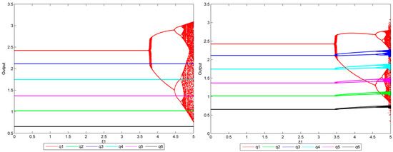
Figure 29.
The bifurcation diagram of ((left): = 0, (right): = 0.4).
From Figure 30, when = 0 (left), the system remains in equilibrium regardless of . When are at 1.5 (right), the system is stable, as is below 2.440. Then, there is a small interval, and in this interval the production of all enterprises is unstable. When the value increases to 2.455, the system is no longer balanced and transitions from stable to double-cycle to chaos.
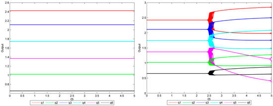
Figure 30.
The bifurcation diagram of ((left): = 0, (right): = 1.5).
Figure 31 and Figure 32 show the Lyapunov exponents for Figure 29 and Figure 30. When = 0 and = 3.750 (left in Figure 31), the system shows bifurcation. When > 4.690, the maximum Lyapunov exponent changes from negative to positive, and the system is in chaos. When are 0.4 and = 3.440 (right in Figure 31), bifurcation appears and then all enterprises bifurcate. When > 4.810, the maximum Lyapunov exponent changes from negative to positive, and the system becomes chaotic.
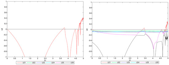
Figure 31.
The Lyapunov exponent diagram ((left): = 0, (right): = 0.4).
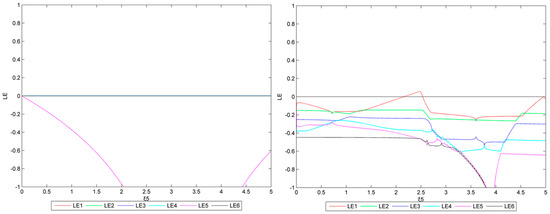
Figure 32.
The Lyapunov exponent diagram ((left): = 0, (right): = 1.5).
When are 0 (left in Figure 32), the maximum Lyapunov exponent is always negative. When equal 1.5 (right in Figure 32) and ranges from 2.160 to 2.455, the maximum Lyapunov exponent changes from negative to positive, and there are bifurcations in various regions. When > 2.455, the maximum Lyapunov exponent is no longer positive, while the system becomes a double-cycle.
4.3. Discussion
Different from the author’s previous research, this paper calculates the changes in the imbalance situation, stable regions, bifurcation diagrams, and Lyapunov index in China’s steel market under multiple emission reduction policies and multiple emission reduction targets, and then makes corresponding comparisons. This paper does not discuss the optimal output strategy. Only the aforementioned three scenarios were analyzed.
It should be pointed out that the dynamic production decision-making model proposed in this paper is a basic theoretical model, which takes the overall social welfare function as the objective function, and is composed of enterprise–profit function, production function, cost function, emission reduction target, and multiple emission reduction scenarios. It can be applied to many countries and regions and many industrial sectors, and also has strong universality. Subsequent representations of bounded rational strategies in the model, differences in production strategies in different regions, and changes in stability domains under different emission reduction targets can all be replaced and calculated using different parameters. However, in essence, this model is an ideal and relatively simple optimization model. Because of certain assumptions in the model, there were some gaps between the calculations and the actual results, but some trends and rules can still be found and identified.
From the calculation results, it can be found that the optimal output obtained by the output selection model of the steel industry is the equilibrium output under the condition of market stability, and the optimal output is also consistent with the current basic distribution of China’s steel industry. That is to say, the optimal output in North China, East China, and Central and South China is much larger than that in other regions, and its impact on the market and production adjustment strategies has always been the focus of government departments. In other regions, because of its low market share, the impact on the market is not obvious.
For the optimal output of the model, the author’s previous research has carried out detailed calculations; this paper does not discuss these, but focuses instead on the impact of the adjustment of bounded rational production strategies in various regions of the steel market.
In general, the introduction of a bounded rationality policy will not directly affect the optimal output of enterprises, because it is the intermediate process behavior of enterprises, but changes in the production adjustment strategy of enterprises will directly affect the stability of the steel market. If market stability ceases to exist, there is no need to discuss optimal production decisions for firms.
Whether the enterprise has a large output or a small output, excessive production adjustment strategies will affect the stability of the market. However, the possibility of market imbalance is very small (the unit of production adjustment strategy in this paper is 100 million tons, which is almost impossible for enterprises and is almost completely “unreasonable” only for more obvious and outstanding results and calculations). Therefore, for enterprises, the research on the combination of carbon emission reduction goals and carbon emission reduction strategies affects the production decisions of enterprises to a certain extent. The existence of the carbon trading benchmark affects the Nash equilibrium output of the steel market. According to the calculation, under the scenario of more stringent emission reduction targets and greater production adjustment strategies (very unlikely), the lower the carbon trading benchmark, the smaller the stability range, and the change is not obvious in other cases.
For North China, East China, and Central South China, since their steel production bases will not be fundamentally relocated and eliminated for a long period of time in the future, their market share will still occupy a considerable proportion of the whole. From the calculation results, the increase in CO2 emission reduction targets increases the production adjustment strategy of these regions, that is, they can adopt more flexible production plans. Obviously, under the dual carbon goal, it is most important for steel enterprises in these regions to complete the corresponding emission reduction plans (the requirements of the emission reduction policy combination can be ignored to a certain extent).
For the northeast, southwest and northwest regions, although the possibility of market imbalance is also less, it cannot be ruled out that, due to the low market share and poor profits of these enterprises, the decision-makers of these enterprises may undertake “life-threatening” expansion of production, and the final result will cause market imbalance. Of course, in most cases, the production adjustment plans of the steel enterprises in the northeast, southwest, and northwest regions are relatively stable. Therefore, under the dual carbon goal, for steel enterprises in the northeast, southwest, and northwest regions, implementing a simple combination of CO2 emission reduction policies is more conducive to market stability and the realization of emission reduction goals.
5. Conclusions and Recommendations
With the proposal of China’s “dual carbon” goal, the steel market not only has to deal with the pressure brought by the ever-changing trade environment and industrial transformation and upgrading, but also the issue of CO2 emission reduction, which has become a major problem that the steel market must face. There are increasing calls to implement various emission reduction policies, such as carbon trading policies and product subsidy policies, but it is unreasonable to only consider meeting emission reduction targets while ignoring market production stability. In order to examine the comprehensive impact of carbon trading policies and product production adjustment strategies on the steel market, this paper constructs a repeated dynamic game model. This paper introduces a carbon trading mechanism and bounded rationality expectation strategy. Then, this paper analyzes the output selection and market stability of steel oligarchs under multiple emission reduction targets, multiple CO2 emission benchmarks and policies, and further analyzes and compares the dynamic production adjustment and market imbalance conditions of steel oligarchs under various conditions, as well as the corresponding stability regions, bifurcation diagrams, and Lyapunov exponents. This research draws the following conclusions.
- When the steel industry implements a single or mixed carbon trading policy and output adjustment policy, without considering emission reduction targets, the system balance influence of larger output enterprises is much greater than that of smaller output enterprises. When larger output enterprises adopt weak positive adjustment policies, smaller output enterprises will have more autonomy in output planning. However, when large-scale enterprises adopt improper output adjustment policies, such as excessive output, it is more dangerous for small-scale enterprises, which will cause their output adjustment space to shrink sharply. In addition, when multiple firms simultaneously employ dynamic output adjustments, the system is more prone to falling into an imbalanced state;
- When output adjustment policy and a single carbon trading emission reduction policy are combined to act on the steel market, as emission reduction targets are gradually raised, the adjustment policies that enterprises with larger or smaller outputs can implement will show an increasing trend, that is, enterprises can implement more output adjustment policies without causing the system to fall into a state of bifurcation or even chaos;
- If the emission reduction target consistently raised, and the carbon trading policy adds subsidies, CCS, and other mixed emission reduction policies, the enterprises are affected. For enterprises with a larger output, even if a more complex mixed emission reduction policy appears, as the target gradually increases, the output adjustment policies that can be implemented will also show an increasing trend. However, for enterprises with a smaller output, the output adjustment policy will be restricted and affected by more factors, including emission reduction targets. The rule of change is different from that of the single carbon trading scenario, and even occurs that the stability zone shrinks and the output adjustment policies decrease when the emission reduction target is large. This means that enterprises with smaller outputs need to be more cautious in formulating their own production plans to ensure that the enterprises and the entire steel market will not fall into a state of imbalance;
- The selection of the benchmark value will not cause significant changes in the stability region of the steel market. However, it is still recommended that relevant departments should not adopt too aggressive emission reduction targets and benchmarks when considering the implementation of the carbon trading mechanism.
Carbon trading and output adjustment strategies have their own reasonable scope of application. The government and enterprises should carefully weigh these strategic issues in their output plans. The government and enterprises need to consider all factors and differences of enterprises when formulating future production plans. Enterprises with larger outputs and a larger market share can take more flexible choices in the process of output adjustment; however, enterprises with smaller outputs and a smaller market share should not adjust output plans significantly in the process of output adjustment and should observe the output changes in enterprises with larger outputs and make corresponding adjustments. When the steel industry implements more stringent emission reduction targets and mixed policies in the future, the government should pay close attention to the adjustment of production plans of various enterprises (especially those with small outputs) at any time, and be aware of malicious production, disruption of market competition order, and market imbalance.
Although this paper studies the impact of carbon trading policies and product production strategies on the steel market, and reaches the above conclusions, there are still certain limitations and areas that need to be improved, which will also become important directions for future research These are as follows: (1) Most of the data used in this paper come from the statistical yearbook data published by the national or provincial governments, and the companies studied are actually approximations of regional steel statistical data. This is due to the large number of the steel enterprises in China, and the country has not yet established a complete enterprise-level statistical system, so there is an insufficient grasp of enterprise data. (2) This paper adopts the bounded rational strategy for the decision-making behavior of enterprises but, in fact, the decision-making process of enterprises is a rather complicated process, the strategy may also be changed or even canceled, and the game competition process between enterprises is more complex and fiercer, which will cause the model to change. The dynamic game production model established in this paper is still an idealized basic model, which also has certain limitations.
Therefore, in the future research process, whether it is related to China or other countries and regions, it is necessary to continue to increase data mining and analysis, and to build more accurate theoretical models by obtaining enterprise-level production, energy consumption, CO2 emissions, and other data. In addition, the characterization of the decision-making process of enterprises, the production game process between enterprises, and the decomposition process of emission reduction targets between the government and enterprises should receive more in-depth and multi-situational discussion, and a more universal theoretical model should be established, so as to be applicable to empirical research in a wider area and a more common industry.
Author Contributions
Conceptualization, D.L. and Y.D.; methodology, Y.D.; software, H.W. and Y.D.; validation, Q.D. and Y.D.; formal analysis, H.W. and Y.D.; investigation, Y.D.; resources, Y.D.; data curation, Y.D.; writing—original draft preparation, D.L. and Y.D.; writing—review and editing, Q.D., H.M. and Z.H.; visualization, Q.D. and Y.D.; supervision, Y.D.; project administration, Y.D.; funding acquisition, Y.D. All authors have read and agreed to the published version of the manuscript.
Funding
The authors gratefully acknowledge the financial support from the Social Science Foundation of Liaoning Province [L19CJY006]. These will be used for the purchase and collection of information and data, as well as for the modification and publication of the manuscript.
Institutional Review Board Statement
Not applicable.
Informed Consent Statement
Not applicable.
Data Availability Statement
The statistics in this paper are from the China Statistical Yearbook, China Industrial Statistical Yearbook, China Energy Statistical Yearbook, China Steel Yearbook, and the statistical yearbooks of various provinces. All data are publicly available on the website and can also be purchased. The relevant results of this paper are calculated on the basis of these public data, and these statistical data and books have been marked and quoted in the paper.
Acknowledgments
The author of this paper thanks the School of Geography of Liaoning Normal University for their assistance in developing this research.
Conflicts of Interest
The authors declare no conflict of interest.
References
- Smale, R.; Hartley, M.; Hepburn, C.; Ward, J.; Grubb, M. The impact of CO2 emissions trading on firm profits and market prices. Clim. Policy 2006, 6, 31–48. [Google Scholar] [CrossRef]
- Allevi, E.; Gnudi, A.; Konnov, I.V.; Oggioni, G. Decomposition method for oligopolistic competitive models with common environmental regulation. Ann. Oper. Res. 2013, 268, 441–467. [Google Scholar] [CrossRef]
- Boutabba, M.A.; Lardic, S. EU Emissions Trading Scheme, competitiveness and carbon leakage: New evidence from cement and steel industries. Ann. Oper. Res. 2017, 255, 47–61. [Google Scholar] [CrossRef]
- Stuhlmacher, M.; Patnaik, S.; Streletskiy, D.; Taylor, K. Cap-and-trade and emissions clustering: A spatial-temporal analysis of the European Union Emissions Trading Scheme. J. Environ. Manag. 2019, 249, 109352. [Google Scholar] [CrossRef] [PubMed]
- Hanclova, J.; Zapletal, F.; Smid, M. On interaction between carbon spot prices and Czech steel industry. Carbon Manag. 2020, 11, 121–137. [Google Scholar] [CrossRef]
- Karali, N.; Xu, T.F.; Sathaye, J. Reducing energy consumption and CO2 emissions by energy efficiency measures and international trading: A bottom-up modeling for the US iron and steel sector. Appl. Energy 2014, 120, 133–146. [Google Scholar] [CrossRef]
- Yamazaki, M. Effects of CO2 Emissions Trading on Steel Scrap Recycling: A Simulation Analysis Using a Computable General Equilibrium Model. Mater. Trans. 2011, 52, 498–506. [Google Scholar] [CrossRef]
- Kushwaha, S.; Ghosh, A.; Rao, A.K. Collection activity channels selection in a reverse supply chain under a carbon cap-and-trade regulation. J. Clean. Prod. 2020, 260, 121034. [Google Scholar] [CrossRef]
- Zhu, L.; Zhang, X.B.; Li, Y.; Wang, W.X.; Guo, J. Can an emission trading scheme promote the withdrawal of outdated capacity in energy-intensive sectors? A case study on China’s iron and steel industry. Energy Econ. 2017, 63, 332–347. [Google Scholar]
- Zhao, Y.B.; Wang, C.; Sun, Y.W.; Liu, X.B. Factors influencing companies’ willingness to pay for carbon emissions: Emission trading schemes in China. Energy Econ. 2018, 75, 357–367. [Google Scholar]
- Wei, L.; Chen, W.D.; Yang, Y. Decision-makings on the Scrap Iron and Steel Remanufacturing Considering the Introduction of Carbon Emission Reduction Investment. Ind. Eng. Manag. 2018, 23, 65–71+79. [Google Scholar]
- Liu, X.; Li, Y.; Zhang, D.Y.; Zhu, L. On the Effectiveness of the Abatement Policy Mix: A Case Study of China’s Energy-Intensive Sectors. Energies 2018, 11, 559. [Google Scholar] [CrossRef]
- Dai, H.C.; Xie, Y.; Liu, J.Y.; Masui, T. Aligning renewable energy targets with carbon emissions trading to achieve China’s INDCs: A general equilibrium assessment. Renew. Sustain. Energy Rev. 2018, 82, 4121–4131. [Google Scholar] [CrossRef]
- Zeng, B.X.; Zhu, L. Market Power and Technology Diffusion in an Energy-Intensive Sector Covered by an Emissions Trading Scheme. Sustainability 2019, 11, 3870. [Google Scholar] [CrossRef]
- Lin, W.B.; Gu, A.L.; Liu, B.; Wang, Z.X.; Zhou, L.L. Carbon market, sector competitiveness and carbon leakage: Steel sector case. Progress. Inquisitiones Mutat. Clim. 2019, 15, 427–435. [Google Scholar]
- Duan, Y.; Han, Z.L.; Zhang, H.; Wang, H.Y. Research on the applicability and impact of CO2 emission reduction policies on China’s steel industry. Int. J. Clim. Chang. Strateg. Manag. 2021, 13, 352–374. [Google Scholar] [CrossRef]
- Zhang, C.; Zhang, X.X. Evolutionary game analysis of air pollution co-investment in emission reductions by steel enterprises under carbon quota trading mechanism. J. Environ. Manag. 2022, 317, 115376. [Google Scholar] [CrossRef] [PubMed]
- Zhu, B.Z.; Jiang, M.X.; He, K.J.; Chevallier, J.; Xie, R. Allocating CO2 allowances to emitters in China: A multi-objective decision approach. Energy Policy 2018, 121, 441–451. [Google Scholar] [CrossRef]
- Pang, T.; Zhou, S.; Deng, Z.; Duan, M.S. The influence of different allowance allocation methods on China’s economic and sectoral development. Clim. Policy 2018, 18, 27–44. [Google Scholar] [CrossRef]
- Zhang, Y.L.; Gu, L.Y.; Guo, X. Carbon audit evaluation system and its application in the iron and steel enterprises in China. J. Clean. Prod. 2020, 248, 119204. [Google Scholar] [CrossRef]
- Jiang, T.Y.; Song, J.C.; Yu, Y. The influencing factors of carbon trading companies applying blockchain technology: Evidence from eight carbon trading pilots in China. Environ. Sci. Pollut. Res. 2022, 29, 28624–28636. [Google Scholar]
- Wei, P.B.; Cui, H.R.; Gang, M.Q. Scenario analysis of energy conservation and CO2 emissions reduction policies in China’s iron and steel sector. Pol. J. Environ. Stud. 2017, 26, 2307–2317. [Google Scholar] [CrossRef]
- Duan, Y.; Han, Z.L.; Mu, H.L.; Yang, J.; Li, Y.H. Research on the impact of various emission reduction policies on China’s iron and steel industry production and economic level under the carbon trading mechanism. Energies 2019, 12, 1624. [Google Scholar] [CrossRef]
- Li, Z.L.; Dai, H.C.; Song, J.N.; Sun, L.; Geng, Y.; Lu, K.Y. Assessment of the carbon emissions reduction potential of China’s iron and steel industry based on a simulation analysis. Energy 2019, 183, 279–290. [Google Scholar] [CrossRef]
- Zhu, X.H.; Zeng, A.Q.; Zhong, M.R.; Huang, J.B.; Qu, H.P. Multiple impacts of environmental regulation on the steel industry in China: A recursive dynamic steel industry chain CGE analysis. J. Clean. Prod. 2019, 210, 490–504. [Google Scholar] [CrossRef]
- Wang, P.; Dai, H.C.; Ren, S.Y.; Zhao, D.Q.; Masui, T. Achieving Copenhagen target through carbon emission trading: Economic impacts assessment in Guangdong Province of China. Energy 2015, 79, 212–227. [Google Scholar] [CrossRef]
- Wu, R.; Dai, H.C.; Geng, Y.; Xie, Y.; Mosui, T.; Tian, X. Achieving China’s INDC through carbon cap-and-trade: Insights from Shanghai. Appl. Energy 2016, 184, 1114–1122. [Google Scholar] [CrossRef]
- Zhang, Y.J.; Shi, W.; Jiang, L. Does China’s carbon emissions trading policy improve the technology innovation of relevant enterprises? Bus. Strategy Environ. 2020, 29, 872–885. [Google Scholar] [CrossRef]
- Zhang, Y.J.; Wang, W. How does China’s carbon emissions trading (CET) policy affect the investment of CET-covered enterprises? Energy Econ. 2021, 98, 105224. [Google Scholar] [CrossRef]
- Tan, Q.L.; Liu, L.T.; Zhu, S.L. Study on the benchmark method for national carbon trading in China’s iron and steel industry. Progress. Inquisitiones Mutat. Clim. 2021, 17, 590–597. [Google Scholar]
- Tan-Soo, J.S.; Li, L.L.; Qin, P.; Zhang, X.B. Do CO2 emissions trading schemes deliver co-benefits? evidence from shanghai. Clim. Policy 2021, 22, 64–76. [Google Scholar] [CrossRef]
- Meinel, U.; Schule, R. The Difficulty of Climate Change Adaptation in Manufacturing Firms: Developing an Action-Theoretical Perspective on the Causality of Adaptive Inaction. Sustainability 2018, 10, 569. [Google Scholar] [CrossRef]
- Safarzynska, K.; Van den Bergh, J.C.J.M. A higher rebound effect under bounded rationality: Interactions between car mobility and electricity generation. Energy Econ. 2018, 74, 179–196. [Google Scholar]
- Rezvani, Z.; Hudson, P. How do middle managers really make decisions within the oil and gas industry? Saf. Sci. 2021, 139, 105199. [Google Scholar] [CrossRef]
- Hammond, S.F.; Gajendran, T.; Savage, D.A.; Maund, K. Unpacking the problems behind the limited green construction adoption: Towards a theoretical model. Eng. Constr. Archit. Manag. 2021, 28, 833–844. [Google Scholar]
- Ji, W.Z. Study on Outputs Game Models and Chaotic Characters in Electric Power Oligopoly. Ph.D. Thesis, Tianjin University, Tianjin, China, 2008. [Google Scholar]
- Sun, Z.H.; Ma, J.H. Game Model of Dynamically Repeated Price in Domestic Steel Market. J. Xidian Univ. 2009, 19, 43–47. [Google Scholar]
- Tu, H.L. Research on the Dynamics of the Cournot Dynamical Game Models in the Electricity Market and the Renewable Resource Market. Ph.D. Thesis, Tianjin University, Tianjin, China, 2013. [Google Scholar]
- Dang, J.F.; Hong, I.H. The equilibrium quantity and production strategy in a fuzzy random decision environment: Game approach and case study in glass substrates industries. Int. J. Prod. Econ. 2013, 145, 724–732. [Google Scholar] [CrossRef]
- Tan, Z.L.; Liang, Z.X. Study on Dynamic Repetition Game Model of Coal Market Price in China. Coal Econ. Res. 2016, 36, 45–48. [Google Scholar]
- Di, X.; Liu, H.X.; Ban, X.J. Second best toll pricing within the framework of bounded rationality. Transp. Res. Part B Methodol. 2016, 83, 74–90. [Google Scholar]
- Di, X.; Liu, H.X.; Zhu, S.; Levinson, D.M. Indifference bands for boundedly rational route switching. Transportation 2017, 44, 1169–1194. [Google Scholar] [CrossRef]
- Liu, L.W. Nonlinear Complex Dynamics of Carbon Emission Reduction Cournot Game with Bounded Rationality. Complexity 2017, 2017, 8301630. [Google Scholar]
- Yu, Y. Complexity Analysis of Taxi Duopoly Game with Heterogeneous Business Operation Models and Differentiated Products. J. Intell. Fuzzy Syst. 2017, 33, 3059–3067. [Google Scholar]
- Ding, M.; Qian, Y.; Zhang, J.; He, J.; Yi, J. Defence model based on multistage dynamic game with consideration of bounded rationality against power system cascading failure. Electr. Power Autom. Equip. 2017, 37, 69–74+82. [Google Scholar]
- Zhang, J.X. Study on Competitive Game Model with Bounded Rationality Enterprise of Emissions Trading. Value Eng. 2018, 6, 101–103. [Google Scholar]
- Sang, H.Y.; Xie, X.L.; Wang, B. Ship scheme selection based on decision maker’s limited rationality. J. Dalian Marit. Univ. 2019, 45, 58–64. [Google Scholar]
- Zhang, Y.M.; Chen, W.D.; Mi, Y. Third-party remanufacturing mode selection for competitive closed-loop supply chain based on evolutionary game theory. J. Clean. Prod. 2020, 63, 121305. [Google Scholar]
- Wu, F. Research on Dynamic and Complexity of Energy-Saving Investment about Multichannel and Multienergy Supply Chain. Complexity 2020, 2020, 2409636. [Google Scholar]
- Duan, Y.; Han, Z.L.; Mu, H.L.; Yang, J.; Li, Y.H. Research on the Influence of Bounded Rationality and Product Differentiation on the Stability of Steel Industry Market. Discret. Dyn. Nat. Soc. 2020, 2020, 1828674. [Google Scholar]
- Fan, B.; Guo, T.T.; Xu, R.Z.; Dong, W.Q. Evolutionary Game Research on the Impact of Environmental Regulation on Overcapacity in Coal Industry. Math. Probl. Eng. 2017, 2021, 5558112. [Google Scholar] [CrossRef]
- Ma, J.H.; Hou, Y.M.; Wang, Z.X.; Yang, W.H. Pricing strategy and coordination of automobile manufacturers based on government intervention and carbon emission reduction. Energy Policy 2021, 148, 111919. [Google Scholar]
- Huang, Q.Y.; Wang, J.W.; Ye, M.W.; Zhao, S.M.; Si, X. A Study on the Incentive Policy of China’s Prefabricated Residential Buildings Based on Evolutionary Game Theory. Sustainability 2022, 14, 1926. [Google Scholar] [CrossRef]
- Li, X.J.; Wang, C.; Kassem, M.A.; Liu, Y.S.; Ali, K.N. Study on Green Building Promotion Incentive Strategy Based on Evolutionary Game between Government and Construction Unit. Sustainability 2022, 14, 10155. [Google Scholar] [CrossRef]
- NBS (National Bureau of Statistics of the People’s Republic of China). China Statistical Yearbook 2005–2017; The Editorial Board of China Statistical Yearbook: Beijing, China, 2005–2017. Available online: http://www.stats.gov.cn/tjsj/ndsj/ (accessed on 2 September 2022).
- NBS (National Bureau of Statistics of the People’s Republic of China). China Industrial Economy Statistical Yearbook 2005–2017; The Editorial Board of China Industrial Economy Statistical Yearbook: Beijing, China, 2005–2017. Available online: https://navi.cnki.net/knavi/yearbooks/YZGJN/detail (accessed on 2 September 2022).
- NBS (National Bureau of Statistics of the People’s Republic of China). China Energy Statistical Yearbook 2005–2017; The Editorial Board of China Energy Statistical Yearbook: Beijing, China, 2005–2017. Available online: https://navi.cnki.net/knavi/yearbooks/YCXME/detail?uniplatform=NZKPT (accessed on 2 September 2022).
- CISA (China Iron and Steel Association). China Steel Yearbook 2005–2017; The Editorial Board of China Steel Yearbook: Beijing, China, 2005–2017. Available online: http://www.csdri.com.cn/periodical (accessed on 2 September 2022).
- IPCC (Intergovernmental Panel on Climate Change). IPCC Guidelines for National Greenhouse Gas Inventories; IPCC: Bracknell, UK, 2006. [Google Scholar]
- Duan, Y.; Mu, H.L.; Li, N. Analysis of the relationship between China’s IPPU CO2 emissions and the industrial economic growth. Sustainability 2016, 8, 426. [Google Scholar] [CrossRef]
- Färe, R.S.; Grosskopf, C.A.; Pasurka, J. Environmental production functions and environmental directional distance functions. Energy 2007, 32, 1055–1066. [Google Scholar] [CrossRef]
- Lee, J.D.; Park, J.B.; Kim, T.Y. Estimation of the shadow prices of pollutants with production/ environment inefficiency taken into account: A nonparametric directional distance function approach. J. Environ. Manag. 2002, 64, 365–375. [Google Scholar] [CrossRef] [PubMed]
- Guenno, G.; Tiezzi, S. The Index of Sustainable Economics Welfare (ISEW) for Italy; Fondazione Eni Enrico Mattei: Milano, Italy, 1998. [Google Scholar]
Publisher’s Note: MDPI stays neutral with regard to jurisdictional claims in published maps and institutional affiliations. |
© 2022 by the authors. Licensee MDPI, Basel, Switzerland. This article is an open access article distributed under the terms and conditions of the Creative Commons Attribution (CC BY) license (https://creativecommons.org/licenses/by/4.0/).

