Abstract
Carbon emission reduction (CER) is increasingly becoming a global issue. This study explored the impact mechanism of upgrading of consumption structure (UCS) and human capital level (HC) on carbon emissions, and an empirical test was carried out using the provincial panel data from 2000 to 2019 in China. The results show the following: (1) China’s UCS could significantly curb carbon emissions. (2) At present, China’s HC is positively correlated with carbon emissions. The higher the level of human capital, the less conducive to CER. Additionally, the moderating effect of HC could inhibit the CER induced by UCS. (3) Regional heterogeneity analysis showed that the UCS in the central and western regions of China was conducive to CER, while the estimated coefficient of UCS on CER in the eastern region was not significant. (4) The UCS could reduce carbon emissions by stimulating the mediating effect of industrial upgrading. Based on empirical study results, this study proposes policy suggestions that can help reduce China’s carbon emissions.
1. Introduction
Due to the high carbon emissions induced by China’s rapid economic growth and extensive development, China is facing enormous pressure to reduce carbon emissions [1]. In 2021, China ranked first in carbon dioxide emissions (11.9 billion tons), accounting for about 33% of the global total and 1.7 times that of Europe and the United States combined [2]. Since the United Nations Climate Conference in 2009, CER has become an issue for China’s economic development [3]. At the 75th United Nations General Assembly in 2020, President Xi Jinping stated that China would increase its independent contribution to CER. China would adopt more powerful policies and measures to reach the CO2 emission peak by 2030, reduce CO2 emissions per unit of GDP by 60–65% compared to 2005, and achieve carbon neutrality by 2060 [4]. Therefore, determining how to achieve CER is increasingly becoming an important academic research topic.
According to the assessment report of the United Nations Intergovernmental Panel of Experts on Climate Change (IPCC), carbon dioxide emissions caused by human activities are the leading cause of global warming [5]. Studies have shown that about 72% of the global carbon emissions are from household consumption [6], and the proportion of Chinese residents’ CO2 emissions out of the total CO2 emissions is as high as 40~50% [7]. The consumption structure of residents affects the efficiency and level of carbon emissions. It can be said that the change in the consumption structure determines whether China can achieve the goal of CER as scheduled and whether it can achieve low-carbon economic development [8,9].
Due to China’s decades of economic development and investment in education, residents’ HC has been greatly improved. As of 2020, the gross enrollment rate of higher education in China has increased from 12.5% in 2000 to 54.4% in 2020, and the average number of years of education for the working-age population has increased to 10.8 years. With the improvement of consumers’ HC, consumption preference, income level, and consumption pattern all change, which further affects the consumption structure of residents and regulates its impacts on carbon emissions. Therefore, what role the improvement of HC plays in the effects of UCS on carbon emissions is a question worth discussing.
Therefore, in this empirical study, the CO2 emission data from 30 provinces in China were used to construct a fixed-effects model to test the impacts of UCS on CO2 emissions, and the mechanism was analyzed. Additionally, the role of HC in the impacts of UCS on carbon emissions was also determined. The objectives were to (1) include carbon emissions, HC, and UCS in a analytical framework to explore the moderating role of HC in the impacts of UCS on CO2 emissions; (2) divide the 30 provinces into three groups (the eastern region, the central region, and the western region) to explore the heterogeneity in the impacts of UCS and HC on CO2 emissions; (3) use a mediation model to explore the impact of UCS on CO2 emissions, to provide a new perspective for studying the relationship between UCS and CO2 emissions. This study provides specific theoretical basis for policy makers to carry out CER and promote China’s green and high-quality development.
2. Literature Review
Previous studies studied the impacts of consumption on carbon emissions in two major ways. The first is to decompose the influencing factors of carbon emissions and then estimate the role of consumption. For example, Yang et al. used the LMDI decomposition method to decompose carbon emissions in China and found that the consumption per capita was an important influencing factor of CO2 emissions [10]. Yin et al. [11] found that the significant increase in the consumption of urban residents led to an increase in direct and indirect carbon emissions by using the nested input–output model. Fan et al. [12] used the structural decomposition analysis (SDA) model to study the influencing factors of Beijing’s carbon footprint and found that the consumption per capita was the main driving factor in the indirect increase in Beijing’s carbon footprint. Wang et al. also used the SDA to study the factors that affect the indirect carbon emissions of residents in the Beijing–Tianjin–Hebei region and found that the level of residents’ consumption was the main factor affecting the indirect carbon emissions [13]. Shao et al. combined the multi-scale input–output method with SDA to analyze the driving force of carbon emissions in Shanghai and found that the change in consumption per capita was the main driving factor for the growth in carbon emissions [14]. Zou [15] used the LMDI decomposition method to analyze the indirect energy consumption for residents’ carbon emissions in Guangzhou and found that the residents’ consumption structure had a stimulating effect on the CO2 emissions induced by indirect energy consumption of Guangzhou’s urban and rural residents. Zhang et al. [16] used a multi-regional input–output model to study the trends and differences in carbon emissions from consumption in China and found that China’s CO2 emissions caused by consumption were gradually increasing. Yuan et al. [17] and Wang et al. [18] used a structural decomposition analysis model to examine the impact of China’s consumption on the indirect CO2 emissions of residents. They found that the rise in consumption per capita played a leading role in the growth in residents’ indirect carbon emissions, and limiting residents’ carbon emissions was vital in controlling total carbon emissions.
Other scholars mainly used econometric methods to study the impact of consumption on carbon emissions. For example, Zhu et al. [19] found that China’s household consumption positively affected carbon emissions by using the ridge regression econometric model. Li et al. [20] conducted a study by using the cointegration model based on the data from 1978 to 2009 of China. They found that the increase in China’s total consumption significantly increased the total carbon emissions, and after 2003, the impact of residents’ consumption on carbon emissions gradually increased. Zhou et al. [21] analyzed the relationship between Chinese residents’ consumption structure and carbon emissions using a spatial econometric model and concluded that the UCS could significantly reduce carbon emission intensity. Luo [22] constructed the stochastic impacts by regression on population, affluence, and technology (STIRPAT) model based on Chinese provincial panel data and found that the UCS had a positive effect on CER. Li et al.’s study based on a modified STIRPAT model found that the impact of primary energy consumption structure on carbon emissions was very significant [23]. Lin [24] studied the drivers of CO2 emissions in Ghana using an autoregressive distributed lag model and found that the change in energy consumption structure from biomass to petroleum fuel was the main driving factor for the increase in CO2 emissions in Ghana. However, there is still a lack of research on the impacts of UCS on carbon emissions and the mechanism.
At present, academic research conclusions on the relationship between HC and carbon emissions have not yet reached a consensus. Some scholars believe that the improvement of HC can help curb carbon emissions. For example, Fleisher et al. [25] reported that the improvement of HC could promote the development of a low-carbon economy by improving total factor productivity. Xu et al. [26] found that technological progress caused by the improvement of HC reduced CO2 emissions. Xi et al. [27] studied the impact of innovative human capital on CO2 emissions in China and found that innovative human capital inhibits environmental degradation in China. Li and Ullah Sana [28] show that the improvement of HC reduced the CO2 emissions of the BRICS countries. Yin et al. [29] explored the relationship between HC and CO2 emissions in 101 countries and found that the improvement of HC was conducive to CER. Wang and Xu [30] empirically analyzed the relationship between HC and CO2 emissions based on panel data from 70 countries and found that HC was an important driving factor for the development of a low-carbon economy. Hao et al. [31] showed that the improvement of HC could reduce CO2 emissions in G7 countries. However, some study authors believe that the improvement of HC will promote carbon emissions or that there is a non-linear relationship between the two. For example, Li [32] showed that the improvement of HC in China increased the CO2 emissions after 1992. Rahman et al. [33] found that both economic growth and human capital improvement deteriorated the environmental quality of newly industrialized countries in the long run. Awaworyi et al. argued that the improvement of HC contributed to economic growth, but it negatively impacted CO2 emissions [34]. Dou [35] and Yao et al. [36] believed that the improvement of HC had an uncertain impact on CO2 emissions, making the relationship between HC and CO2 emissions present an inverted U shape.
At present, there is no report on the impacts of HC and UCS on carbon emissions. However, it is necessary to explore the relationship among UCS, HC, and carbon emissions. Therefore, in this study, the UCS, HC, and carbon emissions were included in the research framework. Based on the empirical analysis of the provincial panel data in China, the impact mechanism of UCS and HC on carbon emissions was clarified. The results of this study will have certain theoretical and practical significance.
3. Materials and Methods
3.1. Theory and Research Hypothesis
With the UCS, residents will prefer high-quality, healthy, low-energy, and environment-friendly goods and services, so UCS is beneficial for the development of a low-carbon economy [37]. In addition, the UCS from goods consumption to service consumption increases the proportion of the service industry, which has environmentally friendly features such as low pollution and low energy consumption, and plays an active role in reducing energy consumption per unit of product [38]. That is, the development of service industry is beneficial to reducing carbon emissions. On the other hand, with the UCS, residents’ pursuit of higher-quality products and services will lead to innovations in products and technologies, and low-carbon and environmental friendly production technologies will be applied on a large scale, thereby reducing carbon emissions on the supply side. Based on the above analysis, this study proposed the following hypothesis:
Hypothesis 1.
The UCS helps reduce carbon emissions.
HC can adjust the strength or direction of the impact of UCS on CER by affecting the UCS. This is reflected in that the generally improved human capital can enhance the innovation and skill of laborers, which is beneficial to technological upgrading [39]. Technological upgrading will enhance product quality, reduce energy consumption, and promote the consumption of more environmentally friendly high-quality products and services, which is conducive to CER. In addition, with the improvement of HC, residents’ income will increase, which will promote residents to upgrade their consumption structure and drive the prosperity of the service market, thus reducing carbon emissions.
On the other hand, the improvement of HC has an effect on income [40]. HC is the basic element for residents to obtain labor remuneration. Studies have shown that income level is positively related with HC [41]. The improvement of consumers’ HC and the increase in income will promote consumers’ pursuit of a higher quality of life. Under the influence of the Diderot effect, more affluent consumers will strive to maintain cross-cultural consistency when consuming goods [42]. Consumers often change the consumption patterns they followed in the past and act in pursuit of specific product brands and product quality, which strengthens conspicuous and comparative consumption. This change will inevitably increase resource and energy consumption, which is not conducive to CER [43]. Moreover, due to the increasing of purchasing power, consumers will accelerate the frequency of commodity replacement in the process of UCS, artificially shortening the service life of commodities, resulting in substantial waste of resources and energy, which is not conducive to CER. Based on the above analysis, this study proposed the following hypotheses:
Hypothesis 2.
HC can strengthen the impact of UCS on CER.
Hypothesis 3.
HC can restrain the impact of UCS on CER.
If the UCS is beneficial to CER, then what is the impact mechanism of the UCS on CER? Industrial upgrading can spawn more green, low-carbon, and high-tech industries and high-quality service industries, thereby reducing carbon emissions. This has been confirmed by scholars’ research [44,45,46]. The demand-induced driving force for industrial upgrading is the UCS. With the UCS, consumers’ demands gradually shift from goods consumption to service consumption, which will eventually promote industrial upgrading. According to the relevant theories of economics, the UCS can lead to the upgrading of industries in the following two ways: (1) Engel effect. With the growth in residents’ income, the share of the commodities with low income elasticity of demand, such as food, will gradually reduce in the total demand, while the share of these with high income elasticity of demand, such as services, will gradually increase. This change caused by the UCS gradually upgrades the industrial structure [47], optimizes resource allocation, and improves production efficiency. It can be said that the UCS has induced industrial upgrading, which is conducive to CER. (2) Baumol effect. With the UCS, the demands for high-end products and services in line with the UCS will increase, which will drive increase in the return on capital and increase in productivity of related industries. To adapt to the changes in the consumption structure, capital will flow into related industries, which will lead to further expansion of the scale of high-end manufacturing and high-end service industries. The industrial structure will develop in the advanced direction, that is, the traditional industries will be replaced gradually by emerging industries with low pollution, low energy consumption, and high added value, which will be more conducive to CER [48]. Based on the above analysis, it can be considered that the UCS can reduce carbon emissions through the indirect impact of industrial upgrading. Therefore, the following hypothesis was made.
Hypothesis 4.
The UCS can reduce carbon emissions through the mediating effect of industrial upgrading.
3.2. Model Construction and Variable Selection
3.2.1. Panel Regression Model
The impact, population, affluence, and technology (IPAT) equation was proposed and used earlier in the research on human activities and the environment [49]. It quantifies the impact of economic activities on the environment based on three key elements: technological progress, economy, and population. However, the IPAT equation has limitations such as constant elastic coefficient, so Dietz et al. [50] proposed the stochastic impacts by regression on population, affluence, and technology (STIRPAT) model (I = αPβAγTδ). For convenience, it is necessary to perform dimensionless processing on the variables. After taking the logarithm of the model, Formula (1) was obtained:
where I represents environmental impact; i and t denote individuals and time, respectively; P represents the influence of population factors; A represents the level of economic development; T represents technical efficiency; a and u denote a constant term and a random error term, respectively; β, γ, and δ are the elastic coefficients of independent variables.
This study expanded the framework of the STIRPAT model and choose the CO2 emissions per capita (C) as the proxy variable of environmental pressure, the urbanization level as the proxy variable of population factor, the gross domestic product (GDP) as the proxy variable of economic development level, and the industrialization rate (IND) as the proxy variable of technology level. Considering that the topic of this study is the influences of UCS and HC on carbon emissions, the UCS and HC were used as independent variables, and the multiplication term of the two was introduced to examine whether HC had a moderating effect. Previous studies have shown that population density (DENS), openness level (OPEN), and innovation level (INNOV) all have an impact on carbon emissions [22,51]. Therefore, DENS, OPEN, and INNOV were included in the model. Authors of previous studies believe that there may be a nonlinear relationship between GDP and CO2 emissions. Therefore this study introduced the square term of C into the equation to test whether there was a Kuznets’ “Inverted U-shaped” nonlinear relationship between GDP and CO2 emissions. Based on the above analysis, we can obtain the following model by modifying Formula (1):
where i represents the province, t represents the year, βi are the parameters to be estimated, and ɛ is the stochastic disturbance.
3.2.2. Mediation Model
Compared with regression analysis, mediation analysis can more accurately analyze the process and mechanism of the influence between variables and obtain more in-depth research results [52]. In the mediation model, the mediating variable represents an internal mechanism and plays a mediating role in the impact of the independent variable on the dependent variable. On the basis of the direct impact of the independent variable X on the dependent variable Y, the mediating variable M is added, which is equivalent to an internal transmission medium through which X has an indirect effect on Y [52,53]. The relationship among X, Y, and M can be represented by the following regression equations:
where X is the independent variable, M is the mediating variable, and Y is the dependent variable. The coefficient c in Equation (3) is the total effect of X on Y, the coefficient a in Equation (4) is the effect of X on M, the coefficient b in Equation (5) represents the effect of M on Y after controlling the effect of X, and the coefficient c’ represents the direct effect of X on Y after controlling the effect of M. Thus, c = ab + c’, where c is the total effect, c’ is the direct effect, and ab is the mediating effect (indirect effect).
According to the mediation model construction method and the theoretical analysis of the indirect influence mechanism above, the carbon emissions per capita was taken as the explained variable, the UCS was taken as the core explanatory variable, and the industrial upgrading was used as the mediating variable to construct the mediation model and thereby reveal the indirect influence between UCS and carbon emission. The mediation model was constructed as follows:
where lnC represents carbon emissions per capita, lnUCS represents the upgrading of consumption structure, M represents the level of industrial upgrading, CONTROL is a series of control variables, and αi, βi, and γi are parameters to be estimated. The meanings of other variables are the same as the previous ones.
3.2.3. Data Sources
This study collected panel data (2000~2019) of 30 provinces in China, for the data of some provinces were missing. According to the methods proposed by IPCC [54] and Wang et al. [55], the CO2 emissions of each province can be regarded as the product of the CO2 emission factor for each energy combustion and the energy combusted in each province [56]. According to the regional energy consumption data over the years, the CO2 emissions of each province were calculated.
where i is the energy type, E is the physical consumption of the i-th energy, the unit for natural gas is ton of standard coal/10,000 m3, and the units for the other energy types are kg standard coal/kg. The unit for carbon emissions coefficient is t carbon/t standard coal. The conversion coefficient Θ of each energy (standard quantity) was from the China Energy Statistical Yearbook, and the carbon emission coefficient Ψ of each energy was from IPCC [54]. The conversion coefficients and carbon emission coefficients of the 8 types of energy are shown in Table 1.

Table 1.
Standard conversion coefficient and carbon emission coefficient of each energy.
The core explanatory variable was the UCS. Most previous studies on consumption structure were based on the commodity structure classified according to the household consumption function by the National Bureau of Statistics, including food/tobacco/alcohol, clothing, housing, daily necessities/services, transportation/communication, education/entertainment, medical care, and others [57]. Additionally, they reported that the three classes of non-material consumption including transportation/communication, education/entertainment, and health care, were flexible. This indicates that the consumption of these three types will increase with the increase in income, and their shares in the total expenditure will increase, which reflects the upgrading trend of consumption structure [58]. Therefore, by referring to the previous research results, this study selected transportation/communication, education/entertainment, and health care as high-level consumption, and their proportions in the total consumption were calculated to measure the level of UCS.
In this study, the average years of education of employed persons were used to measure the regional HC [59]. The educational level of the employed was divided into five categories, namely illiterate, primary school, junior high school, high school, and junior college and above, and the years of education were 0, 6, 9, 12, and 13 years, respectively.
where Li represents the proportion of the labor force with the ith category of education level in the total labor force. The raw data were obtained from the China Labor Statistics Yearbook.
Control variables included: GDP per capita (GDP) (total GDP divided by total population), GDP per capita squared, urbanization level (URBAN) (proportion of urban population in the total population), DENS (ratio of population to land area), IND (ratio of the added value of the secondary industry to total output), OPEN (ratio of total import and export to GDP), and INNOV (ratio of three types of patent applications received to the population).
The mediating variable is the level of industrial upgrading (M). Drawing on the research results of Xu and Jiang [60], the industrial structure hierarchy coefficient was introduced as a proxy indicator of M.
where qi is the proportion of the output value of the i-th industry.
Then, the logarithm of the calculation result was taken as the mediating variable.
Data were obtained from China Statistical Yearbook, China Science and Technology Statistical Yearbook, China Industrial Statistical Yearbook, and Wind database (2001~2020). Some missing data were supplemented by provincial statistical yearbooks and related websites or complemented by the linear interpolation method. Descriptive statistics of the variables are shown in Table 2.
Table 2.
Descriptive statistics of variables.
4. Empirical Results and Analysis
4.1. Regression Analysis
The STATA software version 16.0 and Formula (2) were used to analyze the whole set of data. Before performing model estimation, Hausman’s test was performed to determine whether to use fixed effects or random effects. The Hausman’s test results (Table 3) showed significance at the 1% level. This indicates that it is more scientific and reasonable to use the fixed-effects model for estimation. Therefore, in this study, the fixed-effects (FE) model was used as the main regression model, and the OLS mixed regression and random-effects (RE) regression results were selected as references.
Table 3.
Benchmark regression analysis.
The estimation results of the fixed-effects regression (Model (2)) (Table 3) show that the estimated coefficient of lnUCS was −5.847 (p < 1%). This indicates that the UCS has a significant inhibitory effect on C. The change in the UCS rate per unit could lead to a reduction of 5.847 units of C. The OLS mixed regression (Model (1)) results show that the coefficient of lnUCS was −4.633 (p < 5%), and the RE regression (Model (3)) results show that the coefficient of lnUCS was −4.946 (p < 1%). Both coefficients were significantly negative, which is consistent with that of the fixed-effects model. Thus, the hypothesis H1 is verified, that is, the UCS is conducive to CER.
This study further investigated whether there was a significant relationship between the HC and CO2 emissions per capita. The results show that the estimated coefficients of lnHC of Model (1), Model (2), and Model (3) were 3.639, 3.255, and 2.834, respectively (p < 1%). This indicates that in the time series examined, the HC has a significant role in promoting carbon emissions.
To clarify the mediating role of HC in the impact of UCS on carbon emissions, this study introduced the cross-product term of lnHC and lnUCS into the model. The FE regression (Model (2)) results show that the regression coefficient of the cross-product term of HC and UCS on C was positive (p < 1%). The estimation results of Model (1) and Model (3) also show that the coefficient of the cross-product term of lnHC and lnUCS was a positive value (p < 1%). This indicates that the improvement of HC can significantly reduce the carbon emissions caused by UCS. Thus, the hypothesis H3 is verified.
According to the estimation results of Model (2), GDP had a promoting effect on carbon emissions among the control variables (p < 1%). The coefficient of the quadratic term of GDP was negative (p < 1%). This indicates that the impact of GDP on carbon emissions has a Kuznets’ inverted U-shaped characteristic. The fixed-effect (Model (2)) analysis results show that the regression coefficients of the DENS (p < 1%) and IND (p < 1%) on carbon emissions were positive. This indicates that the two have a promoting effect on carbon emissions. The OPEN and INNOV have inhibitory effects on carbon emissions (p < 1%). The higher the OPEN and INNOV, the more conducive to CER.
4.2. Analysis of Regional Heterogeneity
Due to the regional differences in economic and social development, there are differences in income and consumption culture. Therefore, the consumption structure and carbon emission levels of different regions are also different. To further investigate the difference in the impact of UCS on carbon emissions in different regions, this study divided the 30 provinces into the eastern (11 provinces), central (8 provinces), and western (11 provinces) regions according to the characteristics of regional economic development, geographical conditions, and population distribution (Figure 1) [61]. Then, empirical analysis was conducted to test the specific impact of UCS on carbon emissions in the eastern, central, and western regions based on Formula 2. Before performing model estimation, the Hausman’s test was used to determine whether to use fixed-effects regression or random-effects regression. According to the Hausman test result (Table 4), it is more reasonable to use fixed-effects regression. The mixed regression (Model (1)) and the RE regression (Model (3)) results show that the UCS in the eastern region had a significant inhibitory effect on carbon emissions. However, the FE regression (Model (2)) result shows that the impacts of the UCS and HC in the eastern region on carbon emissions were not significant. Therefore, it is impossible to judge whether the UCS in the eastern region is conducive to CER.
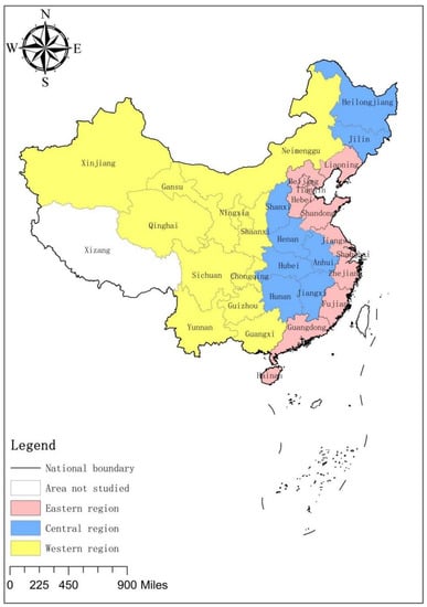
Figure 1.
Schematic diagram of the division of the study area.
Table 4.
Regression results for the eastern, central, and western regions.
The FE regression results (Model (5)) show that the regression coefficient of the UCS in the central region on CO2 emission per capita was −11.448 (p < 1%). Additionally, the OLS mixed-regression result (Model (4)) and the RE regression result (Model (6)) also show that the coefficients were significantly negative. This indicates that the UCS is conducive to CER in the central region. The FE regression result (Model (8)) shows that the regression coefficient of UCS in the western region on CO2 emission per capita was −9.461 (p < 1%), and the OLS mixed-regression result (Model (7)) and the RE regression result (Model (9)) also show that the coefficients were significantly negative. Therefore, the UCS is also conducive to CER in the western region.
According to the FE regression result (Model (2)), the effect of the HC in the eastern region on carbon emissions was not significant. Therefore, it is impossible to judge whether the HC in the eastern region is conducive to promoting carbon emissions. According to the FE regression result (Model (5)), the regression coefficient of the HC in the central region on carbon emissions was 6.590 (p < 1%). This indicates that the improvement of the HC will significantly increase carbon emissions in the central region. According to the RE regression result (Model (8)), the regression coefficient of the HC in the western region on carbon emissions was 5.351 (p < 1%). This indicates that the improvement of the HC will also significantly increase carbon emissions in the western region. In general, the regression results of the impact of HC on carbon emissions in the central and western regions are in good agreement with the regression result based on the overall sample.
According to the FE regression result (Model (2)), the regression coefficient (−0.960) of the cross-product term of lnHC and lnUCS on carbon emissions was not significant in the eastern region. Therefore, it is impossible to judge the role of HC in the eastern region in the impact of the UCS on CER. According to the FE regression result (Model (5)), the regression coefficient of the cross-product term of lnHC and lnUCS on carbon emissions was 5.256 (p < 1%). This indicates that the improvement of the HC is not conducive to the inhibition effect of the UCS on carbon emissions in the central region. According to the FE regression result (Model (8)), the regression coefficient of the cross-product term of lnHC and lnUCS on carbon emissions was 4.611 (p < 1%). This indicates that the improvement of the HC in the western region has a certain inhibition on the effect of the UCS on CER.
4.3. Robustness Tests
To examine whether the above conclusions about the impact of UCS on carbon emissions are robust, the following robustness tests were performed.
4.3.1. Dynamic Analysis Using Generalized Method of Moments (GMM)
Since carbon emission is a constantly changing process, the impact of UCS on carbon emissions has a certain lag effect. Based on Equation (2), this study introduced the first-order lag term of C as an explanatory variable to investigate its dynamics. The estimation model was constructed using the system-generalized method of moments (SYS-GMM) and the difference-generalized method of moments (DIF-GMM). At the same time, the validity of the instrumental variables and estimated results was tested by using the following two methods proposed by Arellano and Bover [62]. One is the serial correlation test, including Arellano–Bond (1) and Arellano–Bond (2) tests, which are used to discriminate whether there is autocorrelation in the stochastic disturbance term of the model. The null hypothesis is that there is no autocorrelation in the stochastic disturbance term of the difference equation. When the test result is that there is no serial correlation, the model estimation result is valid. The other is the Sargan test, which is mainly used to judge whether the instrumental variables are effective as a whole. The null hypothesis is that the instrumental variables in the model are effective. The test results (Table 5) show that the p-values of the Arellano–Bond (1) test of each model were all less than 0.1, and the p-values of the Arellano–Bond (2) test and Sargan test were all greater than 0.1. This indicates that the modelling settings are reasonable. The estimation results in Table 5 show that regardless of whether SYS-GMM estimation (p < 1%) or DIF-GMM (p < 1%) estimation was used, the regression coefficient of UCS on carbon emissions were all negative. This is consistent with the conclusion obtained by baseline regression.
Table 5.
Dynamic regression results.
4.3.2. Replacing Explained Variables with Carbon Emission Intensity
In this study, carbon emission intensity (CO2 emissions per unit of GDP) was also used as an explained variable for estimation. The FE regression (Model (2)), OLS mixed regression (Model (1)), and RE regression (Model (3)) results (Table 6) show that the regression coefficients of the UCS on carbon emission intensity were −5.507 (p < 1%), −5.029 (p < 5%), and −4.419 (p < 1%), respectively. This indicates that the UCS also has a significant inhibitory effect on carbon emission intensity. This is consistent with the result obtained in the baseline regression.
Table 6.
Regression results after replacing explained variables with carbon emission intensity.
The FE regression (Model (2)), OLS mixed regression (Model (1)), and RE regression (Model (3)) results show that the regression coefficients of the HC on carbon emission intensity were 3.016, 3.862, and 2.490, respectively (p < 1%). This indicates that the improvement of HC can significantly improve carbon emission intensity. This is consistent with the result obtained in the baseline regression.
The FE regression (Model (2)), OLS mixed regression (Model (1)), and RE regression (Model (3)) results show that the regression coefficients of the cross-product term of lnHC and lnUCS on carbon emission intensity were 2.522, 2.885, and 2.064, respectively (p < 1%). This indicates that the improvement of HC can weaken the inhibitory effect of the UCS on carbon emission intensity. This is also consistent with the result obtained in the baseline regression.
4.4. Mediating Effect Analysis of the Impact of UCS on Carbon Emissions
With the UCS, the industrial structure tends to be upgraded. Thus, it is worth asking: does the advanced industrial structure help the UCS to restrain carbon emissions? To further explore the relationship between UCS and carbon emissions and reveal the transmission mechanism of UCS to carbon emissions, this study used the mediation model to empirically test the mechanism by which the UCS affects carbon emissions on the basis of controlling variables such as HC.
The analysis results of the mediation model according to Formulas (6)–(8) are shown in Table 7. Among them, Model (1) was the estimation using Formula (6), Model (2) was the estimation using Formula (7), and Model (3) was the estimation using Formula (8). The results show that the regression coefficient of UCS on industrial upgrading in Model (2) was positive (p < 5%). This indicates that the UCS can promote industrial upgrading. The regression coefficients of UCS in Model (1) and Model (3) on carbon emissions were both negative (p < 5%), and the coefficient in Model (3) was greater than that in Model (1). This indicates that the UCS can curb carbon emissions. According to the principle of the mediation effect test, it can be seen that the UCS can affect carbon emissions through industrial upgrading. The above results indicate that there is a partial mediation effect on the impact of UCS on carbon emissions, that is, UCS can indirectly positively impact CER by promoting industrial upgrading. Thus, hypothesis H4 is verified.
Table 7.
Estimation results of mediation model.
On the one hand, the UCS is conducive to the introduction of more advanced technology in production, which can improve production efficiency, promote the upgrading of industrial structure, and eliminate backward production capacity. On the other hand, it constantly promotes the replacement of traditional industries by emerging industries with low pollution, low energy consumption, and high added value. This enables the industries to adopt new technologies and new equipment to produce green products, promote the upgrading of products, and construct a green industrial chain. Thus, UCS has a positive effect on CER.
5. Conclusions
CER has already become a global consensus, and countries pay more attention to CER in their development. This study focused on China’s CER and analyzed the impact of UCS on carbon emissions and the mechanism. Taking China’s provincial panel data as an example, the above theoretical mechanisms and research hypotheses were empirically tested. The following conclusions were drawn: (1) The UCS could significantly reduce China’s carbon emissions per capita. (2) At the current stage, the improvement of HC is not conducive to CER. (3) The improvement of HC had an inhibitory effect on the effect of UCS on CER. (4) Regional heterogeneity analysis found that the UCS in the central and western regions was conducive to CER, while the UCS had no significant impact on CER in the eastern region. (5) The mediation effect analysis showed that the UCS could reduce carbon emissions by promoting the mediation effect of industrial upgrading.
In view of the CER induced by UCS, various measures and policies can be taken to promote the upgrading of a reasonable consumption structure, so that the CER target can be realized as soon as possible. Because HC has an inhibitory effect on the CER induced by UCS, it is necessary to improve residents’ scientific consumption concept and reduce the inhibitory effect of HC on the CER induced by UCS, while improving HC. Moreover, in the future development of each region, special attention should be paid to the development of industrial upgrading, and the role of UCS in CER should be strengthened by promoting industrial upgrading.
This study also has certain limitations. Although this study discussed the logical relationship between UCS, HC, and carbon emission, in the face of complex formation factors of carbon emission, more factors should be considered in future research. Additionally, these conclusions are based only on Chinese data. In future research, it is necessary to select more samples from developing countries for comparative research, so that the conclusions of this study could be widely verified.
Author Contributions
Conceptualization, J.D. and M.Z.; methodology, J.D.; software, M.Z.; formal analysis, J.D.; data curation, J.D. and G.C.; writing—original draft preparation, M.Z. and G.C.; writing—review and editing, J.D. and G.C.; supervision, M.Z. All authors have read and agreed to the published version of the manuscript.
Funding
This research was funded by the Zhejiang Province Social Science Planning Project (grant no.17NDJC099YB) and the Zhejiang Soft Science Research Program (grant no.2022C35011).
Institutional Review Board Statement
Not applicable.
Informed Consent Statement
Not applicable.
Data Availability Statement
The series data are mainly from the China Statistics Yearbook, China Statistical Yearbook on Energy, China Labor Statistics Yearbook, Statistics Database of China Economic Information, and China Carbon Accounting Database.
Conflicts of Interest
The authors declare no conflict of interest.
References
- Zhang, J.; Dai, Y.; Su, C.; Kirikkaleli, D.; Umar, M. Intertemporal change in the effect of economic growth on carbon emission in China. Energy Environ. 2021, 32, 1207–1225. [Google Scholar] [CrossRef]
- IEA. Global Energy Review: CO2 Emissions in 2021-Global Emissions Rebound Sharply to highest Ever Level. Available online: https://www.iea.org/data-and-statistics/data-product/global-energy-review-CO2-emissions-in-2021 (accessed on 12 March 2022).
- Yang, X.; Wang, D. Heterogeneous environmental regulation, foreign direct investment, and regional carbon dioxide emissions: Evidence from China. Sustainability 2022, 14, 6386. [Google Scholar] [CrossRef]
- Yang, Y.; Wei, X.; Wei, J.; Gao, X. Industrial structure upgrading, green total factor productivity and carbon emissions. Sustainability 2022, 14, 1009. [Google Scholar] [CrossRef]
- IPCC. Climate change 2013: The physical science basis. In Contribution of Working Group I to the Fifth Assessment Report of the Intergovernmental Panel on Climate Change; Cambrigde University Press: Cambrigde, UK; New York, NY, USA, 2013. [Google Scholar]
- Hertwich, E.; Peters, G. Carbon footprint of nations: A global, trade-linked analysis. Environ. Sci. Technol. 2009, 43, 6414–6420. [Google Scholar] [CrossRef]
- Guan, D.; Hubacek, K.; Weber, C.L.; Peters, G.P.; Reiner, D.M. The drivers of Chinese CO2 emissions from 1980 to 2030. Glob. Environ. Change 2008, 18, 626–634. [Google Scholar] [CrossRef]
- Sun, M.; Chen, G.; Xu, X.; Zhang, L.; Hubacek, K.; Wang, Y. Reducing carbon footprint inequality of household consumption in rural areas: Analysis from five representative provinces in China. Environ. Sci. Technol. 2021, 55, 11511–11520. [Google Scholar] [CrossRef]
- Martínez, M.A.; Cámara, Á. Environmental changes produced by household consumption. Energies 2021, 14, 5730. [Google Scholar] [CrossRef]
- Yang, P.; Liang, X.; Drohan, P.J. Using Kaya and LMDI models to analyze carbon emissions from the energy consumption in China. Environ. Sci. Pollut. Res. Int. 2020, 27, 26495–26501. [Google Scholar] [CrossRef]
- Yin, X.M.; Hao, Y.; Yang, Z.F.; Zhang, L.X.; Su, M.R.; Cheng, Y.H.; Zhang, P.P.; Yang, J.H.; Liang, S. Changing carbon footprint of urban household consumption in Beijing: Insight from a nested input-output analysis. J. Clean. Prod. 2020, 258, 120698. [Google Scholar] [CrossRef]
- Fan, Z.; Lei, Y.; Wu, S. Research on the changing trend of the carbon footprint of residents’ consumption in Beijing. Environ. Sci. Pollut. Res. Int. 2019, 26, 4078–4090. [Google Scholar] [CrossRef]
- Wang, C.; Zhan, J.; Li, Z.; Zhang, F.; Zhang, Y. Structural decomposition analysis of carbon emissions from residential consumption in the Beijing-Tianjin-Hebei region, China. J. Clean. Prod. 2019, 208, 1357–1364. [Google Scholar] [CrossRef]
- Shao, L.; Geng, Z.; Wu, X.F.; Xu, P.; Pan, T.; Yu, H.; Wu, Z. Changes and driving forces of urban consumption-based carbon emissions: A case study of Shanghai. J. Clean. Prod. 2020, 245, 118774. [Google Scholar] [CrossRef]
- Zou, J. Research on carbon emission of residents’ consumption based on the city of guangzhou. Low Carbon Econ. 2017, 8, 31–39. [Google Scholar] [CrossRef]
- Zhang, Y.; Wang, H.; Liang, S.; Xu, M.; Liu, W.; Li, S.; Zhang, R.; Chris, P.N.; Jun, B. Temporal and spatial variations in consumption-based carbon dioxide emissions in China. Renew. Sustain. Energy Rev. 2014, 40, 60–68. [Google Scholar] [CrossRef]
- Yuan, B.; Ren, S.; Chen, X. The effects of urbanization, consumption ratio and consumption structure on residential indirect CO 2 emissions in China: A regional comparative analysis. Appl. Energy 2015, 140, 94–106. [Google Scholar] [CrossRef]
- Wang, Z.; Liu, W.; Yin, J. Driving forces of indirect carbon emissions from household consumption in China: An input–output decomposition analysis. Nat. Hazards 2015, 75, 257–272. [Google Scholar] [CrossRef]
- Zhu, Q.; Peng, X.; Lu, Z.; Yu, J. Analysis model and empirical study of impacts from population and consumptionon carbon emissionsl. Chin. J. Popul. Resour. Environ. 2010, 20, 98–102. (In Chinese) [Google Scholar]
- Li, G.; Zhou, M. Dynamic effects on carbon dioxide emissions of population and consumption: An empirical analysis based on variable parameter model. Popul. Res. 2012, 36, 63–72. (In Chinese) [Google Scholar]
- Zhou, S.; Lin, X. Study on the effect of upgrading consumption structure on carbon emission intensity: Analysis based on provincial spatial panel data model. Ecol. Econ. 2019, 35, 24–29. (In Chinese) [Google Scholar]
- Luo, D.; Shen, W.; Hu, L. Impact of urbanization and consumption structure upgrading on carbon emissions: An analysis based on provincial panel data. Stat. Decis. 2022, 38, 89–93. (In Chinese) [Google Scholar]
- Li, Z.; Li, Y.; Shao, S. Analysis of Influencing factors and trend forecast of carbon emission from energy consumption in China based on expanded STIRPAT model. Energies 2019, 12, 3054. [Google Scholar] [CrossRef]
- Lin, B.; Stephen, D.A. Assessing Ghana’s carbon dioxide emissions through energy consumption structure towards a sustainable development path. J. Clean. Prod. 2019, 238, 117941–117951. [Google Scholar] [CrossRef]
- FLEISHER, B.; Li, H.; Zhao, M.Q. Human capital, econommic growth, and regional inequality in China. J. Dev. Econ. 2010, 92, 215–231. [Google Scholar] [CrossRef]
- Xu, B.; Lin, B.Q. Aquantile regression analysis of China’s provincial CO2 emissions: Where does the differencelie? Energy Policy 2016, 98, 328–342. [Google Scholar] [CrossRef]
- Lin, X.; Zhao, Y.L.; Ahmad, M.; Ahmed, Z.; Rjoub, H.; Adebayo, T.S. Linking innovative human capital, economic growth, and CO2 emissions: An empirical study based on Chinese provincial panel data. Int. J. Environ. Res. 2021, 18, 8503. [Google Scholar] [CrossRef]
- Li, X.Y.; Ullah, S. Caring for the environment: How CO2 emissions respond to human capital in BRICS economies? Environ. Sci. Pollut. Res. Int. 2021, 29, 18036–18046. [Google Scholar] [CrossRef]
- Yin, Y.X.; Xiong, X.R.; Hussain, J. The role of physical and human capital in FDI-pollution-growth nexus in countries with different income groups: A simultaneity modeling analysis. Environ. Impact Assess. Rev. 2021, 91, 106664. [Google Scholar] [CrossRef]
- Wang, J.; Xu, Y.B. Internet usage, human capital and CO2 Emissions: A global perspective. Sustainability 2021, 13, 8268. [Google Scholar] [CrossRef]
- Lin, N.H.; Muhammad, U.; Zeeshan, K.; Wajid, A. Green growth and low carbon emission in G7 countries: How critical the network of environmental taxes, renewable energy and human capital is? Sci. Total Environ. 2021, 752, 141853. [Google Scholar]
- Li, P.; Ouyang, Y.F. The dynamic impacts of financial development and human capital on CO2 emission intensity in China: An ARDL approach. J. Bus. Econ. Manag. 2019, 20, 939–957. [Google Scholar] [CrossRef]
- Rahman, M.M.; Nepal, R.; Alam, K. Impacts of human capital, exports, economic growth and energy consumption on CO2 emissions of a cross-sectionally dependent panel: Evidence from the newly industrialized countries (NICs). Environ. Sci. Policy 2021, 121, 24–36. [Google Scholar] [CrossRef]
- Awaworyi, C.S.; John, I.; Kris, I.; Russell, S. The environmental kuznets curve in the OECD: 1870–2014. Energy Econ. 2018, 75, 389–399. [Google Scholar] [CrossRef]
- Dou, X. Low carbon-economy development: China’s pattern and policy selection. Energy Policy 2013, 63, 1013–1020. [Google Scholar] [CrossRef]
- Yao, Y.; Ivanovski, K.; Inekwe, J.; Smyth, R. Human capital and CO2 emissions in the long run. Energy Econ. 2020, 91, 104907, (prepublish). [Google Scholar] [CrossRef]
- Andersen, M.S.; Massa, I. Ecological modernization-origins dilemmasand future directions. J. Environ. Policy Plan. 2002, 2, 337–345. [Google Scholar] [CrossRef]
- Ge, J.P.; Lei, Y.L. Carbon emissions from the service sector. Clim. Res. 2014, 60, 13–24. [Google Scholar] [CrossRef]
- Yang, G.J.; Wang, F.; Huang, X.H.; Chen, H. Human capital inflow, firm innovation and patent Mix. J. Asian Econ. 2022, 79, 101439, (prepublish). [Google Scholar] [CrossRef]
- Faisal, S.Q.; Abdul, W. Human capital and economic growth: Cross-country evidence from low-middle-and high-income countries. Prog. Dev. Stud. 2013, 13, 89–104. [Google Scholar]
- Valero-Gil, J.N.; Valero, M. Human capital and state income differences in Mexico. Appl. Econ. 2022, 54, 1544–1561. [Google Scholar] [CrossRef]
- Grant, M. Culture and Consumption: New Approaches to the Symbolic Character of Consumer Goods and Activities, Bloomington and Indianapolis; Indian University Press: Bloomington, IN, USA, 1990; p. 123. [Google Scholar]
- Ahmed, Z.; Wang, Z. Investigating the impact of human capital on the ecological footprint in India: An empirical analysis. Environ. Sci. Pollut. Res. 2019, 26, 26782–26796. [Google Scholar] [CrossRef]
- Mi, Z.; Pan, S.; Yu, H.; Wei, Y. Potential impacts of industrial structure on energy consumption and CO2 emission: A case study of Beijing. J. Clean. Prod. 2015, 103, 455–462. [Google Scholar] [CrossRef]
- Wu, L.; Sun, L.; Qi, P.; Ren, X.; Sun, X. Energy endowment, industrial structure upgrading, and CO2 emissions in China: Revisitingresource curse in the context of carbon emissions. Resour. Policy 2021, 74, 102329. [Google Scholar] [CrossRef]
- Tian, X.; Bai, F.; Jia, J.; Liu, Y.; Shi, F. Realizing low-carbon development in a developing and industrializing region: Impacts ofindustrial structure change on CO2 emissions in southwest China. J. Environ. Manag. 2019, 233, 728–738. [Google Scholar] [CrossRef]
- Boppart, T. Structural change and the Kaldor facts in a growth model with relative price effects and non-Gorman preferences. Econometrica 2014, 82, 2167–2196. [Google Scholar] [CrossRef]
- Baumol, W.J. Macroeconomics of unbalanced growth: The anatomy of urban crisis. Am. Econ. Rev. 1967, 57, 415–426. [Google Scholar]
- Ehrlich, P.R.; Holdren, J.P. Impact of population growth. Science 1971, 171, 1212–1217. [Google Scholar] [CrossRef] [PubMed]
- Dietz, T.; Rosa, E.A. Rethinking the environmental impacts of population, affluence and technology. Hum. Ecolo. Rev. 1994, 2, 277–300. [Google Scholar]
- Wang, J.; Luo, X.; Zhu, J. Does the digital economy contribute to carbon emissions reduction? A city-level spatial analysis in China. Chin. J. Popul. Resour. 2022, 20, 105–114. [Google Scholar] [CrossRef]
- Wen, Z.; Zhang, L.; Hou, J.; Liu, H. Testing and application of the mediating effects. Acta. Psychol. Sinica. 2004, 5, 614–620. (In Chinese) [Google Scholar]
- Baron, R.M.; Kenny, D.A. The moderator-mediator variable distinction in social psychological research: Conceptual, strategic, and statistical considerations. J. Pers. Soc. Psychol. 1986, 51, 1173–1182. [Google Scholar] [CrossRef]
- IPCC. 2019 Refinement to the 2006 IPCC Guidelines for National Greenhouse Gas Inventories. Available online: https://www.ipcc-nggip.iges.or.jp/public/2006gl/index.html (accessed on 12 March 2022).
- Wang, D.; He, W.; Shi, R. How to achieve the dual-control targets of China’s CO2 emission reduction in 2030? Future trends and prospective decomposition. J. Clean. Prod. 2019, 213, 1251–1263. [Google Scholar] [CrossRef]
- Zhang, R.; Zhang, C. Does energy efficiency benefit from foreign direct investment technology spillovers? Evidence from the manufacturing sector in Guangdong, China. Sustainability 2022, 14, 1421. [Google Scholar] [CrossRef]
- Li, Y.; Li, Y.; Chen, T.; Hu, Y.Y. Research on the impact of upgrading of consumption structure on energy intensity under the background of urban and rural dual economy. IOP Conf. Ser. Mater. Sci. Eng. 2020, 793, 012058. [Google Scholar] [CrossRef]
- Huang, Z.; Qin, S. The impact of market integration on consumption upgrading: A study based on “Quantity” and “Quality”. Chin. J. Popul. Sci. 2021, 18–31+126. (In Chinese) [Google Scholar]
- Han, W.; Wang, P.; Jiang, Y.S.; Han, H. Nonlinear influence of financial technology on regional innovation capability: Based on the threshold effect analysis of human capital. Sustainability 2022, 14, 1007. [Google Scholar] [CrossRef]
- Xu, M.; Jiang, Y. Can the China’s industrial structure upgrading narrow the gap between urban and rural consumption? J. Quant. Tech. Econ. 2015, 32, 3–21. (In Chinese) [Google Scholar]
- Jin, L.Q.; Wu, H.Y. The regional heterogeneity and countermeasures of china’s carbon emissions. Econ. Manag. 2013, 27, 83–87. (In Chinese) [Google Scholar]
- Arellano, M.; Bond, S. Some tests of specification for panel data: Monte Carlo evidence and an application toemployment equations. Rev. Econ. Stud. 1991, 58, 277–297. [Google Scholar] [CrossRef]

Publisher’s Note: MDPI stays neutral with regard to jurisdictional claims in published maps and institutional affiliations. |
© 2022 by the authors. Licensee MDPI, Basel, Switzerland. This article is an open access article distributed under the terms and conditions of the Creative Commons Attribution (CC BY) license (https://creativecommons.org/licenses/by/4.0/).