Detection Method of End-of-Life Mobile Phone Components Based on Image Processing

Abstract

The number of end-of-life mobile phones is increasing every year, which includes parts that have high reuse values and various dangerous and toxic compounds. An intellectualized and automatic upgrade of the disassembly process of the end-of-life mobile phones would enhance the recycling value as well as efficiency. It would reduce the pollution in the environment. The detection of end-of-life mobile phone parts plays a critical role in automatic disassembly and recycling. This study offers an image processing-based approach for identifying important parts of mobile phones that are nearing the end of their useful lives. An image enhancement approach has been utilized for generating disassembly datasets of end-of-life mobile phones from several brands and models, and different retirement states. The YOLOv5m detection model is applied to train as well as validate the detection model on the customized datasets. According to the results, the proposed approach allows the intelligent detection of battery, camera, mainboard and screw. In the validation set, the Precision, Recall and mAP@.5 are 99.4%, 98.4% and 99.3%, respectively. Additionally, several path planning algorithms are utilized for the disassembly plan of screws which indicates that the genetic algorithm’s use increases the efficiency of disassembly.

1. Introduction

The greatest manufacturer of mobile phones worldwide is China. As per the National Bureau of Statistics of China, from 2015 to 2019, China’s mobile phone production exceeded 1.6 billion units for five consecutive years [1]. Smartphones’ widespread use and quick replacement have led to a dramatic increase in mobile phones that are nearing the end of their useful lives. In 2020, the production of end-of-life mobile phones in China was 550 million units, and the inventory of end-of-life mobile phones was 1 billion units [2]. Improper recycling will lead to the loss of high-value resources (e.g., precious metals, rare earth elements) and the generation of toxic wastes (e.g., mercury, chromium and lead) [3]. As a result, one of the key concerns in the solid waste business is the efficient recycling of outdated mobile phones.

After sorting and disassembly processes, more than 90% of the core components in the retired mobile phones could be extracted and re-used, having a high recycling value [4]. Along with the secondary utilization, mobile phone parts which include the precious and rare metals are crushed and sorted for material recovery. Various metal materials make up 30–40% of the mobile phone’s weight, which includes gold, silver, palladium and other precious metals, and its content is 5–10 times that of ordinary gold concentrate; 40–50% is plastic, approximately 20% is glass [5]. Different methods for removing metal from old mobile phones have been discussed, including pyrometallurgy, hydrometallurgy and biohydrometallurgy [6]. As illustrated in Table 1, about 4.8 tons of metal materials can be obtained from the recycling of 100,000 iPhones [7]. Moreover, the element indium, which is a rare and promising metal, could be extracted from mobile phone screens as well, as the indium extraction efficiency was more than 70% in mobile phone screens [8].

Table 1. The content of recycled metal materials in 100,000 end-of-life iPhones.

Materials	Recycling Weight (kg)	Main Source
Aluminium	1500	Mainboard
Gold	1.1	Mainboard, camera, panel ID, wireless charging coil
Silver	6.3	Mainboard
Rare earth elements	32	Receiver, speaker, camera
Tungsten	83	Touch Engine
Cuprum	1000	Mainboard, receiver, speaker, camera, and panel ID, wireless charging coil
Tin	29	Main board, camera and panel ID
Cobalt	790	Mainboard
Steel	1400	Receiver, touch engine, shell, speaker, camera

Even though end-of-life mobile phones have a tremendous potential for recycling, China currently has relatively low recycling and reuse rates for these devices. The legislation has been drafted, nevertheless, the implementation of regulations on WEEE has been challenging. Furthermore, the pre-treatment and disassembly of retired mobile phones are conducted manually and destructively [9]. Manually disassembling outdated mobile phones is highly costly. In the EU area, the actual market prices for the potentially recoverable materials as well as components of waste mobile phones had not been capable of counterbalancing the costs of manual dismantling according to the European standard labor costs [10]. Owing to the variety of brands and models, retired mobile phones are normally presented with great structural differences. Therefore, automated and intelligent disassembly has enormous promise, particularly for increasing recycling efficiency and reducing resource waste.

1.1. Relevant Research on Recycling End-of-Life Mobile Phones

Solid waste management has grown to be an important issue for national resource reuse and environmental protection because of the negative consequences that solid waste has on the natural environment and human health. Adedeji and Wang [11] suggested an intelligent waste material classification system, which can achieve an accuracy of 87% on the trash image dataset. A machine learning tool with 50-layer residual net pre-train (ResNet-50) Convolutional Neural Network model had been served as the extractor. Moreover, the Support Vector Machine (SVM) was utilized to classify the waste into different types. Deep convolutional neural networks were utilized by Altikat and Gulbe et al. to classify paper, glass, plastic and organic waste [12]. The classification accuracy of four categories of trash using a four-layer and five-layer deep convolutional neural network can achieve 61.67% and 70%, respectively. Zhang and Yang et al. proposed a transfer learning-based waste image classification model [13]. By producing the waste image dataset NWNU-Trash, and based on the deep learning network DenseNet169 pre-trained model, a DenseNet169 model was developed with classification accuracy of 82%. Six screws of various sizes and kinds were detected by Mangold and Steiner et al. using the YOLOv5s and YOLOv5m target detection models [14]. Moreover, the models were verified on the motor automatic disassembly production line. The mAP@.5 and mAP@.5:.95 of the models are 98% and 80%, respectively. Hayashi and Koyanaka et al. suggested an object detection algorithm, which can continuously detect multiple label images at the bottom of discarded cameras. The algorithm identifies the information on manufacturer and camera model name using a template matching the manufacturer’s logo on the label as the template image. The average precision for identification of the manufacturers is 92% [15].

There has been some research on waste management, but very few studies on mobile phones that have reached the end of their useful lives. In 2018, Apple Inc. released a disassembling robot Daisy, which can disassemble nine different iPhones, which reached a disassembling efficiency of 200 iPhones per hour [16]. Huang et al. suggested an enhanced SSD algorithm, in order to detect mobile phone component image targets [17]. The algorithm could better adapt to the detection task of mobile phone components by using deconvolution and using multi-scale transformation. The mAP@.5 of the algorithm hits 78.9% when the picture size is 300 × 300. Cheng et al. proposed a device based on machine vision to automatically disassemble as well as recycle the CPU on the mobile phone circuit board. The device could achieve stable and reliable CPU disassembly and recovery [18]. Tang et al. proposed a multi-scale feature Deep Forest recognition model for smart recycling equipment, which can effectively improve the prediction accuracy and reduce the time cost [19]. Yin et al. developed a five-tuple hybrid graph disassembly model by analyzing information on the structural components of smartphones. A two-population Genetic Algorithm search optimization solution is designed to determine the optimal or suboptimal disassembly sequence solution for smartphones, reducing disassembly time and increasing recovery profit [20].

1.2. Relevant Research on Object Detection Algorithms

Using image processing, machine learning and other technologies, object detection technology locates objects in images or videos. Traditional object detection methods are dependent on the manual extraction of weak features of the target object, which is vulnerable to light as well as background changes. In deep learning, the pixel data of the input images are converted into higher-order abstract-level features, so that the model has stronger representational ability and robustness [21]. Currently, deep learning object detection algorithms have been split into two categories: two-stage and one-stage, according to whether explicit region suggestions are proposed or not. In the created suggested areas, the two-stage object detection technique, like the R-CNN algorithm, converts the object detection issue into a classification problem. The first-stage object detection algorithm has been based on regression, which includes SSD and YOLO algorithm. This category of algorithms does not generate the region of interest and directly carries out the regression task for the entire image.

R-CNN algorithm has a better detection effect as compared to the traditional algorithms, but it has a high cost of time and space because it has low detection efficiency [22]. In 2015, Girshick and Ren et al. respectively suggested Fast R-CNN [23] and Faster R-CNN algorithms, and their mAP on the PASCAL VOC2012 dataset was increased to 68% [24]. High detection accuracy and a clear network are strengths of the SSD method, but the model convergence is slow and unsuitable for small targets [25]. YOLO algorithm has simple network structure and fast detection speed. Nevertheless, its target positioning accuracy is lower as compared to that of the two-stage detection algorithm in the similar period, and unsuitable for small and multiple targets [26].

Currently, object detection algorithms are rapidly developing, specifically the object detection algorithm based on deep learning. It has successfully met the needs of industrial applications by achieving good results in target identification accuracy and detection speed. Moreover, some improved models based on YOLO and SSD, such as YOLOv4 [27], YOLOv5 [28], FSSD [29] and DSSD [30], are suitable for multi-scale and small-target identification problems.

In regard to waste management, the developed object detection algorithms primarily pay attention to the domestic waste classification as well as the detection of a single class of waste. Research on identifying the numerous components included in electrical goods is scarce. Moreover, the current study on end-of-life mobile phones is primarily focused on the physical as well as chemical recycling approaches, especially the extraction of high-value materials. Even if industrial businesses used automation for recycling and end-of-life disassembly, the approach is only suitable for its products. Thus, automated disassembly must be further used for extended products which are from different brands and models as well as various statuses. Despite the fact that the deep learning-based target identification algorithm currently in use has shown positive outcomes, the majority of the training data sets of algorithms still use model data sets, which cannot fully cater to the requirements of practical applications, as well as special data sets that are still required for the recognition and detection of special objects.

In this study, the detection of critical end-of-life mobile phones components is undertaken using image processing technologies. An image enhancement approach has been used to generate disassembly datasets of end-of-life mobile phones from various brands and models, and different retirement states. On the customized datasets, the YOLOv5m detection model is used to train and evaluate the detection model. The result indicates that the proposed approach enables the intelligent detection of battery, camera, mainboard and screw.

2. Research Methodology

2.1. Overview

As illustrated in Figure 1, a dataset of end-of-life mobile phone components was first established by using the steps of key components selection, mobile phone images collection, object annotations, etc. Then, the detection model preparation was completed by selecting an object detection algorithm for training and validation. Moreover, path planning analysis has been carried out for the automated disassembly of a large number of screws. Finally, detection experiments are run for actual situations, and the outcomes of the experiment are examined. Based on the experimental results, the image composition of the custom mobile phone detection dataset as well as the detection model parameters were adjusted to improve the performance of the detection model.

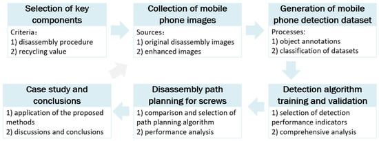
Figure 1. Framework of end-of-life mobile phone component detection.

2.2. Key Components Selection of End-of-Life Mobile Phones

Following the viewpoint of mobile phone structure, there are two categories of mainstream smart phones: Apple structured mobile phones and Android structured mobile phones. Based on the products’ life-cycle data, Apple Inc. could establish an automatic disassembly system through reverse engineering. Hence, this research pays attention to a large number of Android structured mobile phones in the mainstream market. This paper investigates mobile phones’ disassembling process, analyses the recovery value of components and determines the key components, which need to be detected for further disassembly as well recycling processes.

Key components of the disassembling process: With a three-layer construction consisting of the screen, middle frame and back cover, the rear cover of the majority of Android-structured mobile phones is constructed independently from the middle frame. Such smart phone disassembly starts from the back cover, and the disassembly sequence is as follows: back cover–main board cover–camera module–mainboard–auxiliary board–speaker–battery–screen.

The majority of Android-based mobile phones are built in three-step stages, starting from the mainboard and moving on to the battery and the auxiliary board. Because of the variety of brand series and structural designs, automatic disassembly is not technically feasible and economically viable. Therefore, manual disassembly has been primarily adopted. Based on the mobile phone disassembly process diagram, the back cover, screws and camera module are the main structural elements of Android-based mobile phones.

Key components of recycling value: It takes a lot of time and work to disassemble outdated phones completely and without causing any damage. Based on the investigation results of the recycling market, the recycling values of principal components have been shown in Figure 2, among which the recycling value of screen, camera, main board and battery ranks the top. The main board, camera, battery and screen are the most important parts to remove from end-of-life mobile phones based on component recycling value.

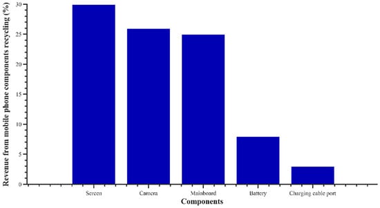
Figure 2. Mobile phone disassembling revenue bar chart.

The back cover, screw, camera, mainboard, battery and screen are main elements in the recycling of mobile phones once their useful lives have ended. Considering the practical disassembling processes and recovery value, the target components chosen in this research involve the battery, mainboard, camera and screws.

2.3. Collection of Mobile Phone Disassembly Images

2.3.1. Capture Original Mobile Phone Image

Based on the production volumes in the Chinese market, representative mobile phone models are chosen for disassembling as well as sampling based on manufacturing numbers in the Chinese market. The samples include ten mobile phones from seven brands (see Table 2), released from 2015 to 2019. In this research, a Hikvsion MV-CE120-10GM CMOS industrial camera was used to collect sample images, with a resolution of 4024 × 3036, and a total of 210 original images were collected. The experimental hardware system is shown in Figure 3.

Table 2. Sample phone brand and model list.

Serial Number	Brand	Model	Release Time	Serial Number	Brand	Model	Release Time
1	Huawei	nova4	2018-11	6	Vivo	X6	2015-11
2	Huawei	nova5pro	2019-6	7	Oppo	A1	2018-4
3	Huawei	7C	2018-3	8	Oppo	A5	2018-7
4	Xiaomi	Xiaomi 4	2016-3	9	Meizu	Noblue 3	2016-6
5	Xiaomi	Redmi note7	2019-1	10	Meizu	Noblue 5	2016-11

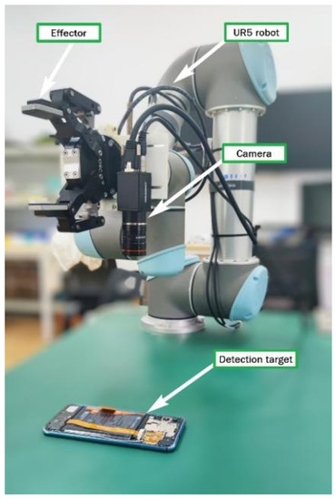
Figure 3. Experimental hardware systems.

Key elements in example photos were annotated using LabelImg, an open-source image annotation programmer [31]. The marked targets are battery, mainboard, camera and screw, numbered 0–3 respectively. The contents to be calibrated include target position and target class. YOLO format has been selected for annotation, which carries five pieces of information regarding each object, including target class, horizontal and vertical coordinate of target center, and target width and height.

In Figure 4, the targets contained in the image are one battery, two cameras and one mainboard, annotating each target information, and the annotation results are shown in Equation (1). Each row in Equation (1) describes a target information in the image. Column 1 is the target class number, represented by c; columns 2 to 5 are the target location information, represented by x, y, w and h, respectively. The data in columns 2 and 3 are the relative coordinates of the target center point in the horizontal and vertical axes; the data in columns 4 and 5 represent the ratio of the length of the target in the horizontal and vertical axes to the length of the whole image, respectively.

$$\left(c x y w h\right)=\left(\begin{array}{c}0\\ 2\\ 2\\ 1\end{array} \begin{array}{c}0.393\\ 0.787\\ 0.843\\ 0.769\end{array} \begin{array}{c}0.502\\ 0.317\\ 0.314\\ 0.500\end{array} \begin{array}{c}0.480\\ 0.061\\ 0.046\\ 0.272\end{array} \begin{array}{c}0.474\\ 0.077\\ 0.063\\ 0.503\end{array}\right)$$

(1)

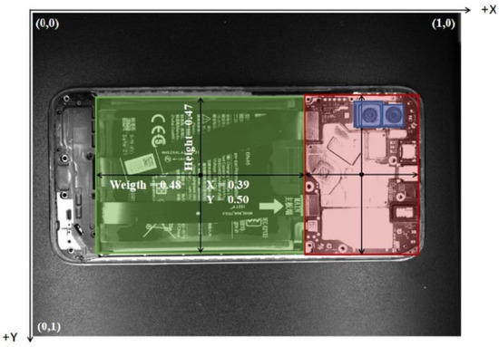
Figure 4. Annotation format for YOLO.

2.3.2. Enhance Original Mobile Phone Image

The original data set was enhanced with images to produce the data set that satisfies the requirements of deep learning’s specifications. By increasing the complexity of data sets and the diversity of targets, the characteristics of mobile phone components in several environments could be obtained for enhancing the robustness of the model. Thus, this research carries out diversified operations on the image, and changes the spatial position of pixels through geometric image enhancement. Picture spatial domain augmentation alters the grey value of pixels in the image. In the process of geometric enhancement, such as translation, scaling, rotation and shear, the transformation equation matrix is shown in Equation (2):

$$\left[\begin{array}{c}x\\ y\\ 1\end{array}\right]=\left[\begin{array}{ccc}{a}_0& a_1& a_2\\ a_3& a_4& a_5\\ 0& 0& 1\end{array}\right]\left[\begin{array}{c}{x}_0\\ y_0\\ 1\end{array}\right]$$

(2)

In different transformations, the values of each parameter in Formula 1 are shown in Table 3. In Table 3, Δx, Δy represent the translation distance of pixel points; s, s_x and s_y represent the scaling ratio in the overall direction and x, y directions respectively; θ represents the rotation angle of pixel points; h represents the offset distance of pixel points; dx, dy represent the proportion of Shear in x and y directions. The effect of the original image after geometric transformation is demonstrated in Figure 5.

Table 3. Geometric transformation matrix parameter list.

	ɑ0	ɑ1	ɑ2	ɑ3	ɑ4	ɑ5
Translation	1	0	Δx	0	1	Δy
Equal scaling	s	0	0	0	s	0
Unequal scaling	sx	0	0	0	sy	0
Clockwise rotation	cos θ	sin θ	0	−sin θ	cos θ	0
Anticlockwise rotation	cos θ	−sin θ	0	sin θ	cos θ	0
Vertical shift	1	0	0	h	1	0
Horizontal shift	1	h	0	0	1	0
Shear	1	dy	0	dx	1	0

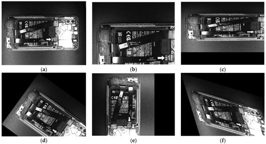
Figure 5. Schematic diagram of image geometric transformation. (a) original image; (b) equal scaling image; (c) unequal scaling image; (d) rotation image; (e) shift image; (f) shear image.

Image spatial domain enhancement, as opposed to picture geometric transformation, which modifies pixel location, directly processes a grey-scale value of images. Specific operations include adding noise, adjusting contrast, adjusting grey level and inverting colours. To simulate an industrial setting with impulsive noise and dust, salt and pepper noise has been included. The exponential transformation method is used in order to adjust the contrast, avoiding the impacts of changes in light intensity. The power transformation technique tries to modify the image’s grey-scale value range. Therefore, the image brightness of the sample has been adjusted to increase the randomness of the image brightness. Moreover, the majority of the mobile phone components are black or white. Use the battery as an illustration. In 10 mobile phones, one phone has a black-brown battery, three have a silvery-white battery, and six phones have pure black batteries. Furthermore, black area images account for most of the disassembled images of mobile phones, and silver-white components, which includes screws and cameras, are embedded in the black body. It is helpful to enhance the model’s recognition of similar parts with different colours and small components such as screws by inverting colours in the images. Figure 6 displays the results of the original image’s spatial domain improvement.

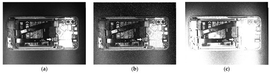
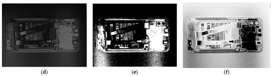
Figure 6. Schematic diagram of image spatial domain enhancement. (a) original image; (b) salt-pepper noise image; (c) grey value increase image; (d) grey value decrease image; (e) adjust contrast image; (f) invert colours image.

To sum up, a variety of geometric enhancement as well as spatial domain enhancement overlay processing were randomly applied to each image (See Figure 7). Four times amplification was performed on 210 original data sets, and YOLO annotation was processed together in the amplification process in order to acquire a data set of 1050 disassembled mobile phone images.

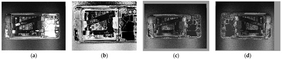
Figure 7. Image enhancement results. (a) original image; (b) image enhancement 1; (c) image enhancement 2; (d) image enhancement 2.

2.4. Generation of End-Of-Life Mobile Phone Data Set

2.4.1. Divide Disassembled Mobile Phones Data Set

Following data screening on the 1050 photos acquired, the images with annotation transformation errors were eliminated. A total of 1022 labelled sample images were obtained, comprising 812 amplified images and 210 original images. Then, the original images and the amplified images were randomly split into training sets Tr1 and Tr2 and validation sets va1 and va2 according to the rate of 8:2, respectively. Tr1 and Tr2 consisted of the complete training set Tr, with a total of 817 images. The whole validation set Va, which contains 205 photos, is made up of the two validation sets Va1 and Va2 (see Figure 8).

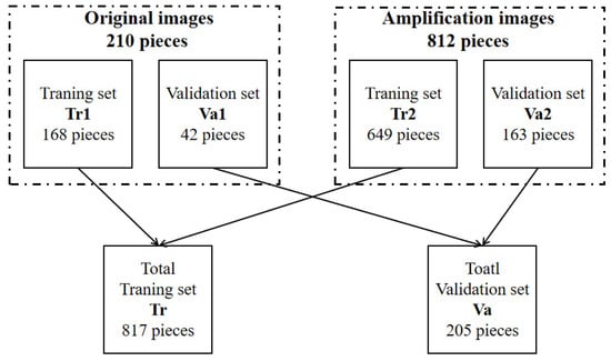
Figure 8. Composition of training set and validation set for mobile phone disassembly images.

In order to verify the robustness of the model, tests have been conducted for images in different scenes and from various sources. The test set of three image groups from three sources was selected, which includes 30 images captured using mobile phones, 30 images enhanced and 20 images in different decommissioning states, respectively. The composition of the test set has been illustrated as Table 4. A total of 30 pictures makes up the test collection of smartphone photos. The collection hardware is a RedmiNote9 mobile phone, and the illumination is an HL-5509 LED lamp. The resolution of images collected is 3264 × 2448, including 26 color images and 6 grey images. Thirty images were randomly selected from the training set for image enhancement, and the image enhancement dataset was constructed. The term “different decommissioning states” describes a variety of severe situations when a mobile phone has been repeatedly dismantled and put back together with the loss of some components. This group of test set images includes two types of images: 10 sample images with both empty screws and non-empty screws and 10 test images composed of component modules.

Table 4. Composition of test set for mobile phone disassembly images.

Type	Piece	Size
images taken by mobile phones	30	(3268 × 2448)
images enhanced	30	(4024 × 3036)
images in different decommissioning states	20	(4024 × 3036)
Total	80	——

Representative images of the three sources have been presented in Figure 9, with different environmental conditions such as clarity, resolution and illumination.

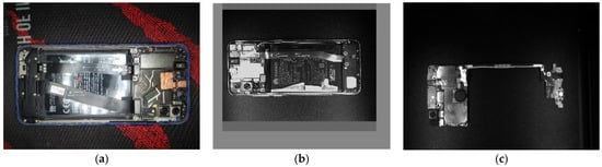
Figure 9. Diagram of images in test set. (a) images taken by mobile phones; (b) images enhanced; (c) images in different end-of-life statues.

2.4.2. Scale and Quantitative Analysis of Dataset

After the data set was divided, the characteristics of objects in the training set Tr were analyzed, and the characteristics of the data set were mined. There are 817 photos in the training set, but they have a high object density (see Figure 10). There are 4466 labelled objects, which includes 502 batteries, 254 mainboards, 730 cameras and 2980 screws. In the four labelled objects, the number of screws is far more than the other three objects, which forms a quantitative imbalance. Moreover, based on the information on the center position and the width and height of object boundary boxes in the training set (see Figure 11), it could be inferred that the dataset contains a large number of small size objects, making the dataset unbalanced at the object scale.

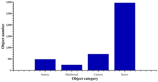
Figure 10. Number of objects in training set.

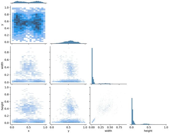
Figure 11. Location and width and height distribution of objects in training set.

2.5. Model Test Indicator

In order to reuse parts and recover materials, this research intends to identify and detect the essential mobile phone components. Therefore, the detection model needed to meet three requirements, including (1) for industrial applications, it needed to ensure the recognition accuracy; (2) real-time detection matters for automatic disassembly and recycling practices; (3) the scale and quantity of targets in the data set vary greatly, and the issue posed by various target sizes must be solved by the model.

Based on deep learning, several object detection algorithms have been proposed in recent years. After preliminary screening, five mature object detection algorithms have been assessed and examined. The mean Average Precision (mAP) and Frames per Second (FPS) are selected as the evaluation indicators in order to evaluate the detection precision as well as detection speed of the model, which have been defined as follows.

2.5.1. mAP

In the object detection task, the intersection over union (IOU) between the actual bounding box of the target object and the model detection bounding box has been utilized for evaluating the accuracy of the bounding box predicted by the model.

The intersection over the union threshold is a predetermined constant and is expressed as $\Omega$. When $IOU>\Omega$, the image in the prediction box has been considered to be a positive sample (containing target objects), or a negative sample (background). Precision (P) and Recall (R) of the object detection model could be calculated based on IOU and $\Omega$, as shown in Equations (3) and (4).

$$Precision=\frac{TP}{TP+FP}$$

(3)

$$Recall=\frac{TP}{TP+FN}$$

(4)

where TP, FP and FN respectively stand for the number of properly projected positive samples, the number of negative samples predicted as positive samples and the number of positive samples incorrectly identified as negative samples. When calculating Precision and Recall, it is generally taken that $\Omega =0.5$. Average Precision (AP) is a commonly utilized indicator in object detection, as shown in Equation (5), where Precision (t) is model Precision when $\Omega =t$.

$$AP={\displaystyle {\int }_0^{1}Precision(t)}\mathrm{d}t$$

(5)

For multi-class object detection tasks, since there may be various different classes of target objects left for detection, the mAP is usually used as the evaluation indicator, and its calculation is as Equation (6):

$$mAP=\frac{{\displaystyle \sum _{n=1}^{N}A{P}_n}}{N}$$

(6)

where N is the number of detection target classes, which in this paper are battery, mainboard and camera as well as screw. AP_n represents AP of the model for the nth target object.

In YOLO object detection, commonly used mAP can be classified into two types based on the $\Omega$:

−

mAP@.5: Multi-class mAP when $\Omega >0.5$;

−

mAP@.5:.95: Average mAP when $\Omega$ from 0.5 to 0.95 in steps of 0.05 in series.

2.5.2. FPS

Frames Per Second (FPS), which refers to the number of images processed by the model per second, is the assessment indicator used to describe the speed of the object identification technique. In object detection, the difference in GPU graphics card greatly influences FPS, so that FPS evaluation of different algorithms needs to be completed on the same hardware system.

2.6. Select Object Detection Model

Five mature object detection algorithms were selected, namely EfficientDet, DSSD, YOLOv4, YOLOv5m and YOLOv5m6, and evaluated on MS COCO2018 dataset. The dataset contained many small size objects and multi-scale objects, which is similar to the characteristics of this paper’s dataset. The graphics card used in the evaluation process was Nvidia GTX 1080Ti, and the statistical data results are shown in Table 5 [28,32,33].

Table 5. Comparison of performance indicators of five models.

Detector	Backbone	FPS	mAP@.5:.95	G
EfficientDet	EfficientNet	24.1	51%	0.770
FSSD	VGGNet	35.7	31.8%	0.627
YOLOv4	CSPDarknet53	36.8	43.5%	0.773
YOLOv5m	Modified CSP v5	56.4	42.5%	0.900
YOLOv5m6	Modified CSP v5	41.6	51%	0.895

For the above five object detection algorithms, a new evaluation indicator G is formulated, and is defined as Equation (7).

$$G=\frac{FP{S}_i}{FP{S}_{\max }}\times k_{FPS}+\frac{mA{P}_i}{mA{P}_{\max }}\times k_{\mathrm{mAP}}$$

(7)

where FPS_i and mAP_i are each model’s performance characteristics, and FPS_max and mAP_max are their maximum values. k_FPS and k_mAP are the indicator weights, and their sum is 1. This paper pays attention to the model detection precision, so k_FPS and k_mAP are 0.4 and 0.6 respectively. After calculation, the G value of each model is shown in the fifth column of Table 5. The YOLOv5m model is chosen for this paper’s identification of mobile phone components since it has the greatest G value. After the above analysis and comparison, in combination with the practical application requirements, it has been determined that the object detection model performance indicator requirements of this project are:

−

mAP@.5 reaches more than 90%,

−

mAP@.5:.95 reaches more than 70%;

−

FPS reaches more than 10 frames per second: the detection speed of each image takes less than 0.1 s.

2.7. Mobile Phone Components Disassembling Path Planning

During the disassembly of mobile phones, the screws are the priority level for disassembly compared to the other three classes of components. In addition, in terms of disassembly time, the screw size is comparatively small, the number is large and the position is scattered, which is the most time-consuming process. Furthermore, compared with batteries, mainboards and cameras in different shapes and sizes, screws would be the most feasible parts for automatic disassembly.

Therefore, the screw is used as the representative component to examine the disassembly path and create the optimal solution of the robot’s moving distance as well as calculate time. The disassembly path planning task of screws requires the robot end-effector to move from the tool magazine, complete the screw disassembly work in one motion, and return to the tool magazine for tool replacement. The essence of this task is a classic Travelling Salesman Problem (TSP), which is for solving the shortest path to each node and returning to the first node given a sequence of nodes and the distance between any two pairs of nodes [34]. Through Improved Circle (IC) [35], Genetic Algorithm (GA) [36] and Ant Colony Optimization (ACO) [37], the path planning of disassembly planning is conducted. Three path planning methods disassembling path length and solution times are compared.

Hamiltonian path is an undirected graph, proposed by the astronomer Hamilton, which goes from a specified starting point to a specified end point, passing through all other nodes and only once on the way, the closed Hamiltonian path is called Hamiltonian cycle. The improved circle (IC) method is also called the successive correction method. The basic idea is to first find a Hamiltonian circle, and then obtain another Hamiltonian circle with smaller weight by appropriate modification, so that the circle weight is reduced. Genetic algorithm (GA) is a stochastic search algorithm that refers to the evolutionary laws of the biological world. The GA mainly simulates the evolution of biological populations through selection, crossover, mutation, etc., and repeats the process several times to continuously update the population genetic factors and select better individuals. When ants forage for food, they leave information hormones on the paths they follow, and the information hormones evaporate over time. The more ants walk along a path, the more information hormones are left behind; in turn, paths with high concentrations of information hormones will attract more ants. The ant colony algorithm solves complex optimization problems by artificially simulating the foraging process of ants (i.e., finding the shortest distance through information exchange and mutual collaboration between individuals).

3. Experiment and Results

The YOLOv5m model for detection was chosen, and the transfer learning method was applied. Because the MS COCO2018 dataset carries a large number of small size objects, as well as the scale difference and quantitative characteristics being close to the dataset of this paper, weights of the MS COCO2018 dataset in YOLOv5m are used as the pre-training weights.

The main parameters in YOLOv5m include:

−

Learning rate (LR): including Initial Learning rate (ILR) and cyclic Learning rate (CycleLR), appropriate suitable LR ensures that the gradient descends correctly and converges to the global optimum.

−

Weights: includes Initial Weights and Weight decay. Weights are used to store updated parameters during model training.

−

Momentum: Momentum eases the change of LR, and helps jump out of optimal local solution by updating iteration with inertia.

−

Batch size: represents the Batch size of image training for each epoch. The performance and speed of the network model may be optimized with an acceptable Batch size.

−

Image size: represents the size of the feature image of the input model. In general, the detection effect is better, but the detection time is longer the larger the feature picture.

Taking the model requirements and hardware performance into consideration, the set values of each parameter in this paper are shown in Table 6.

Table 6. The set values of each parameter.

ILR	CycleLR	Weight Decay	Momentum	Batch Size	Image Size
0.01	0.2	0.0005	0.937	2	1280

The loss of the YOLOv5m includes box loss (L_box), object loss (L_obj) and class loss (L_cls). The total loss (L_total) calculation requires weighted summation of the three types of losses. L_box means the box prediction loss value of the target predicted box from the actual box; L_obj means the confidence prediction loss, which measures whether the target is contained in the prediction box (i.e., whether the background is predicted as the target); L_cls means class prediction loss, which is used to represent the loss of target class prediction error. The weights used in this paper are 0.05, 4.0 and 0.5 respectively, and the total loss has been demonstrated in Equation (8).

$$L_{total}={\displaystyle \sum _i^N(0.05\ast L_{box}}+4\ast L_{obj}+0.5\ast L_{cls})$$

(8)

The platform hardware used in this paper is Intel Core I7-10750H CPU and NVIDIA GeForce RTX 2060 with Max-Q Design GPU. The training platform is Pytorch1.7.0, and CUDA10.1, CuDNN7.6.5 was used for GPU accelerated computation.

3.1. Performance Indicators Updating during Training

Model training had been conducted on the feature map size of 1280 × 1280 input image, as well as training weights based on the MS COCO2018 dataset being used for transfer training, with a total of 300 epochs trained and training for 12 h. Figure 11 depicts the smoothed convergence of the three categories of losses and the overall loss during the training procedure. As shown in Figure 12, the Precision (P), Recall(R) and mAP@.5, mAP@.5:.95 convergence curves with training epochs are smoothed.

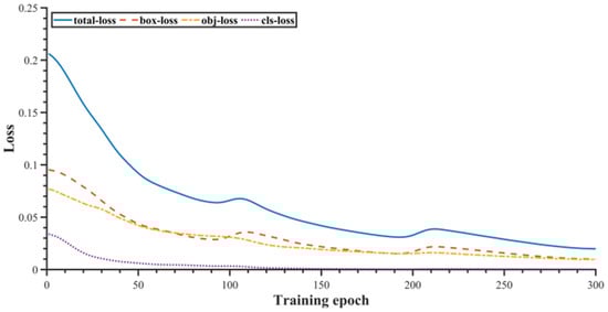
Figure 12. Loss function update curves (smoothing).

During the training process, the class loss stabilized at the 150th epoch and reached convergence, while the box loss and object loss reached stable values at around the 280th epoch, and finally, after 300 epochs of training, the overall loss of the detection model reduced from 0.21 to 0.02 (see Figure 12). The mAP@.5 was the first to achieve a stable value, stabilizing at around 99.3% when the training reached 230 epochs; at about 250 epochs, the model Precision and Recall stabilized at around 99.2% and 98.5% respectively. The training reached 280 epochs and the indicator mAP@.5:.95 tended to converge as well as become stabilized at around 89.5% (see Figure 13).

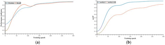
Figure 13. Model performance indicator update curves (smoothing). (a) update curves of Precision and Recall; (b) update curves of mAP.

3.2. Results in Validation Set

The model’s training weights were kept, and the detection model was checked using the validation set. The validation results were shown in Figure 14, and the model performance indicator was shown in Table 7. From a qualitative viewpoint, the trained detection model has good detection performance on the validation set, with larger scale batteries and motherboards being accurately identified and smaller scale cameras being detected as well as located, while the trained model is also competent in detecting challenging screws in terms of number and scale.

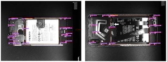
Figure 14. Model evaluation results in validation set.

Table 7. Model performance indicators in validation set.

Class	Images	Labels	P	R	mAP@.5	mAP@.5:.95
Battery	205	141	1	0.993	0.996	0.967
Mainboard	205	67	0.993	0.985	0.995	0.947
Camera	205	194	1	0.993	0.996	0.888
Screw	205	864	0.983	0.964	0.984	0.675
All	205	1266	0.994	0.984	0.993	0.869

In regard to the quantitative analysis of the detection indicators in the validation set, for the four classes of objects to be detected—battery, mainboard, camera and screw—the three detection indicators Precision, Recall and mAP@.5 all exceeded 96%, with these three detection indicators of battery, mainboard and camera all securing over 98%. For the higher threshold detection indication mAP@.5:.95, it was able to get close to 90% for Camera and reached 95 percent for both classes of objects battery and mainboard (96.7 percent for battery and 94.7 percent for mainboard). For screw, the value is lower compared to other classes of objects, reaching 67.5% (see Table 7).

In general, the Precision, Recall and mAP@.5 of the model in the validation set have been higher than 95%, with the three indicators achieving 99.4%, 98.4% and 99.3% respectively, and the mAP@.5:.95 is 86.9%, close to 90%, which satisfies the accuracy requirements of this subject. It was tested on GeForce RTX 2060 with Max-Q Design graphic display platform in regard to the model detection speed, and the detection time of each image was 0.08 s, and the FPS reached 12.5, which satisfied the detection speed requirements of this subject.

3.3. Results in Test Set

Images in the test set are different from those in the training set, which can verify the robustness of the detection model. The object detection model was verified in the test set, and the detection parameters were set as input image size 1280 × 1280, object confidence threshold 0.35, IOU threshold for NMS 0.45 and batch size 1.

On photos captured by mobile phones, the test was run. The image test indicators have been presented in Figure 15. The detection Precision and Recall of the model for battery and camera were more than 90%, and the detection Precision and Recall for screw were more than 85%. Precision and Recall mainboard were 1 and 50% respectively, showing that 50% of mainboard items were not recognized. The overall Precision of the detection model was 94.5%, the Recall was 84.1%, mAP@.5 and mAP@.5:.95 were 83.1% and 57.5%, respectively. Additionally, the model detects an FPS of 12, meaning that each picture took an average of 0.083 s to be detected. In regard to the image enhanced dataset (i.e., the 30 images processed with image enhancement), for the four categories, the detection Precision and Recall can reach more than 90%, while most indicators can reach more than 95%. The overall object detection precision was 99.1%, the Recall was 98%, mAP@.5 and mAP@.5:.95 were 98.4% and 88.1%, respectively (see Figure 16). The model detection FPS was 12.5.

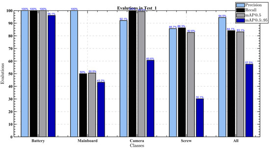
Figure 15. Model performance indicators on the images taken by mobile phones.

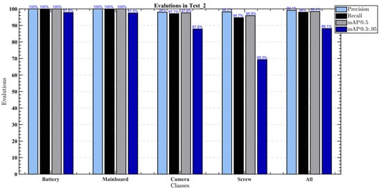
Figure 16. Model performance indicators on the image enhanced dataset.

Various end-of-life mobile phones’ pictures also underwent testing. The Precision, Recall and mAP@.5 of the four detection classes of targets all reached 100%. For mAP@.5:.95, all three detection classes of targets exceeded 90%, except for the lower Screw score of 77.1% (see Figure 17). The detection speed had been consistent with the validation set detection result, and the FPS was 12.5.

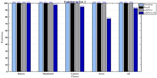
Figure 17. Model performance indicators on the images in different end-of-life statues.

The three kinds of data sets mentioned above were combined to create a new test set for testing, consisting of a total of 80 images, in order to prevent test findings from deviating owing to data sets being too small. The detection parameters were set, e.g., image input feature size was 1280 × 1280, object confidence threshold was 0.40, IOU threshold for NMS was 0.45, and batch size was 1. The model test results have been shown in Table 8. Model detection Precision, Recall, mAP@.5 and mAP@.5:.95 are 97.3%, 93.1%, 93.5% and 74.5%, respectively, in the test set. In the single class object detection, the detection Precision is more than 90%, and the mAP@.5 exceeds 86% for all four classes of objects. Figure 18 displays the outcomes of the detection of the various types of photos in the test set.

Table 8. Model performance indicators in test set.

Class	Images	Labels	P	R	mAP@.5	mAP@.5:.95
Battery	80	53	1	1	1	0.972
Mainboard	80	36	1	0.845	0.866	0.827
Camera	80	101	0.968	0.99	0.992	0.764
Screw	80	491	0.926	0.888	0.881	0.417
All	80	681	0.973	0.931	0.935	0.745

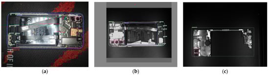
Figure 18. Model evaluation results in test set. (a) images taken by mobile phones; (b) images enhanced; (c) images in different end-of-life statues.

3.4. Comparison of Screw Disassembly Path Planning

Based on the screw detection image samples in the disassembly pictures of end-of-life mobile phones, three path planning algorithms were used. The experiment on performance uses two indicators. One is the screw disassembly path length, as well as the shorter length being preferred. The second indicator is the solving time of the model. In this experiment, ten disassembly images were taken as samples. Using Matlab 2021b software programming, this test experiment was carried out on a computer with an i7-10750h processor, 16G of memory and Windows 10. Related parameters of the Genetic Algorithm (GA) and the Ant Colony Optimization (ACO) are illustrated in Table 9. The test results of three algorithms are shown in Figure 19. The dotted line in the figure represents the disassembly path results of the same mobile phone solved under different algorithms.

Table 9. Parameter table of GA and ACO.

Parameters in genetic algorithm
population	Crossover probability	Mutation probability	Select probability	Maximum iteration
60	0.85	0.12	0.9	80
Parameters in ant colonyoptimization
Ant colony number	Information heuristic factor	Information heuristic factor	Information heuristic factor	Maximum iteration
60	1	5	0.2	40

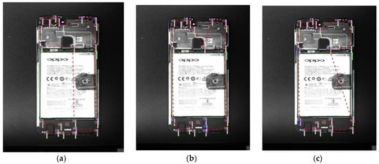
Figure 19. Results of path disassembly in three algorithms. (a) Disassembly path by IC; (b) Disassembly path by GA; (c) Disassembly path by ACO.

The 10 example pictures were solved using the IC, GA and ACO, respectively. The optimal disassembly path distance has been illustrated in Table 10. In regard to the path length, the average path length of IC, GA and ACO was 9580.3 px, 9450.9 px and 9344.4 px, respectively. In the test experiment, the solving time leads to three algorithms which are shown in Table 11. The IC took the shortest time, with an average of 0.02 s. GA took the second place with an average time of 0.13 s, while ACO took the longest with an average time of 0.3 s.

Table 10. Optimal Disassembly path Length of three algorithms (px).

	1	2	3	4	5	6	7	8	9	10	Average
IC	9798	10,702	9289	10,768	8786	8285	10,957	8099	10,177	8942	9580.3
GA	9363	10,297	9968	10,370	8580	8267	10,384	8161	10,177	8942	9450.9
ACO	9363	10,289	9236	10,364	8472	8267	10,384	7950	10,177	8942	9344.4

Table 11. The solving time of the three algorithms (s).

	1	2	3	4	5	6	7	8	9	10	Average
IC	0.131	0.017	0.009	0.007	0.015	0.005	0.006	0.003	0.004	0.004	0.020
GA	0.209	0.156	0.128	0.112	0.127	0.104	0.115	0.113	0.117	0.123	0.130
ACO	0.414	0.319	0.372	0.275	0.305	0.181	0.316	0.191	0.328	0.309	0.301

4. Discussion

4.1. Discussion of Validate Results

The confusion matrix’s findings (see Figure 20) and the model in the validation set show that the mobile phone component detection model is feasible (see Figure 14). The model was able to detect some tiny screw targets that are difficult to notice with the naked eye, especially for the large number of screws with small dimensions. Screws and cameras are the main sources of misclassification. Nevertheless, the largest source of error is false positive detection. Screws and mainboards accounted for 67 percent and 18 percent, respectively, of all false positive detection targets. The proportion of the abovementioned target images in the dataset can be increased to learn information regarding their differences from the background. Furthermore, during validation these false positive errors typically show the lower confidence values provided by the object detectors. Applying confidence thresholds and rejecting discovered objects with low confidence values in a production environment can solve this issue.

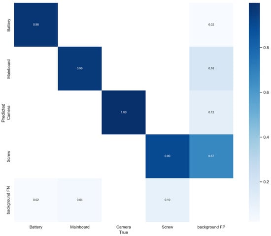
Figure 20. Confusion matrix acquired for detection model on the train set.

In Table 7, the size of the detected item causes a fluctuation in the performance indicator mAP@.5:.95 for object location prediction. For the largest size of batteries, mAP@.5:.95 could reach 0.967, while for the smallest size of screws, only 0.675 could be acquired. In addition, class loss reaches convergence with a lower value earlier (see Figure 12). Indicating that the model finds it more difficult to accurately locate objects and match positive and negative samples than to classify targets, the object loss and box loss converge more slowly and have consistently higher values than class loss. In order to overcome the above issues, improvements could be made in two ways. At first, for the four classes of object scales with large differences, an adaptive anchor clustering operation based on the object scales could be performed before model training for acquiring a suitable series of anchor sizes. Secondly, by optimizing the three types of loss weights in the total loss of Equation (7) and by paying more attention to object loss and box loss for optimization, improved position prediction may be obtained based on the different convergence of the three types of loss functions.

4.2. Discussion of Test Results

For three kinds of data sets from different sources, in contrast to the detection model performance in the validation set, the model’s performance indicators in mobile-phone photos are worse than they are in the validation set, especially for the Recall of mainboards which is merely 50%, indicating that only half of the mainboards have been detected successfully.

In the image enhancement image dataset, the Precise and Recall of the model were 99.1% and 98% respectively, with mAP@.5 above 98% and mAP@.5:.95 achieving 88.1%. This shows that the model is robust to changes in part position and illumination brightness in different image regions for the same image quality.

Environmental factors, which includes illumination, have a relatively large impact on the detection of mainboards. Changing the lighting angle and intensity leads to different detection results even though the mobile phone sample and the sample location posture and detection background were the same (see Figure 21). Comparing the better performance of the model on the validation set indicates that the industrial camera is more robust to imaging under illumination changes as compared to the mobile phone camera and is more suitable for application on industrial production lines.

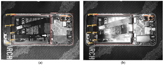
Figure 21. Detection results in images taken by mobile phones. (a) Successfully detected mainboard; (b) Unsuccessfully detected mainboard.

In this collection, screws and other components are consciously mixed in with various photos of the decommissioned state. For instance, negative samples of screws were artificially developed on the phone by removing random screws, which could be easily misclassified. Nevertheless, in the test, the performance of the detection model is still great, with model Precision and Recall reaching 100% with mAP@.5, and mAP@.5:.95 also reached 92%. Performance indicators are 2 to 4 percent higher than the validation set. Because relevant features of the images were learned accurately during the training, after manual processing, the number of objects to be detected per image had been decreased. Furthermore, the dataset of the sample size is relatively small, with only 20 images. Despite the aforementioned factors, the model’s excellent performance shows that it’s capable of correct recognition for a variety of readily mixed samples.

4.3. Discussion of Screw Disassembly Path Planning

Ten images of mobile phone disassembly were taken as samples. Figure 22 shows the results of the disassembly path distance and solution time curves. It could be demonstrated that the distance calculation results of GA and ACO are similar, and they are better than IC. Due to its reduced computation size, IC requires less time to solve a problem than GA and ACO. GA likewise requires less time to solve a problem than AOC. Moreover, the time consumption of IC and GA is relatively balanced. Comparatively, the time consumption of ACO varies considerably across image samples, which is unconducive to the development of production beats in industrial applications. In disassembly path distance and solution time, GA has been balanced and is more suitable for screw disassembly path planning for robot end-effectors.

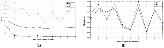
Figure 22. Distance and time curves for different algorithms. (a) Optimal solution distance curve; (b) Solution time curve.

Contrasting the advantages of IC in regard to the solution time, a combination of GA and IC is considered. The IC algorithm is used to determine the initial population code in the GA algorithm, reducing the number of iterations as well as shortening the calculation time of the GA algorithm in disassembly path planning.

5. Conclusions and Future Work

Traditional end-of-life mobile phone recycling and disassembly have low efficiency and high work intensity. This research proposed an intelligent detection approach for end-of-life mobile phone components based on image processing. It provides a theoretical solution for automatic and intelligent disassembly of waste mobile phones in industrial applications.

−

The model was trained and validated using the unique end-of-life mobile teardown dataset, which is based on the YOLOv5m detector. More than 98%, the Precision, Recall and mAP@.5 of model detection were achieved, along with mAP@.5:.95 values of more than 85 percent. On the test data set, the model detection Precision, Recall and mAP@.5 could reach more than 90%, and mAP@.5:.95 could reach more than 70%. The disassembly path planning of screws was successfully carried out using the genetic algorithm, considering the sequence and difficulty in components disassembly.

−

Future research would focus on expanding datasets to improve the performance of the detection model and developing the automatic disassembly station for specific disposed mobile phones.

References

- National Bureau of Statistics of China. Output of Industrial Products. 2022. Available online: https://bit.ly/3aRv03A (accessed on 16 August 2022).
- Deng, M.L.; Du, B.; Fu, Y.G.; Hu, J.Q. Research on the development of recycling and processing of waste mobile. Electr. Appl. 2021, 2, 42–46+54. [Google Scholar] [CrossRef]
- Chai, B.W.; Yin, H.; Wei, Q.; Lu, G.N.; Dang, Z. Relationships between microplastic and surrounding soil in an e-waste zone of China. Environ. Sci. 2021, 42, 1073–1080. [Google Scholar] [CrossRef]
- Song, X.L.; Li, B.; Lv, B.; Chen, Q.; Bai, J.F. Life cycle energy use and carbon footprint of waste mobile phone treatment system. China Environ. Sci. 2017, 37, 2393–2400. [Google Scholar] [CrossRef]
- Qi, Z.D.; Liu, H.J. The mechanical-physical recycling technology for nonferrous metals from waste printed circuit boards. Mater. Rep. 2015, 29, 122–127. Available online: https://bit.ly/3Pbecn3 (accessed on 18 July 2021).
- Tipre, D.R.; Khatri, B.R.; Thacker, S.C.; Dave, S.R. The brighter side of e-waste-a rich secondary source of metal. Environ. Sci. Pollut. Res. 2021, 28, 10503–10518. [Google Scholar] [CrossRef]
- Apple Inc. Apple Environmental Responsibility Report 2019. 14 December 2019. Available online: https://bit.ly/3z8ZxU2 (accessed on 31 March 2022).
- Chugainova, A.A. Efficiency of sorption of metals from electronic waste by microscopic algae. IOP Conf. Ser. Earth Environ. Sci. 2021, 723, 042055. [Google Scholar] [CrossRef]
- Liu, Y.H. Intelligent recognition and disassembly of waste mobile phones: Based on the intelligent recognition of the image of solid waste treatment. J. Jincheng Inst. Technol. 2016, 9, 54–56. [Google Scholar] [CrossRef]
- Bruno, M.; Sotera, L.; Fiore, S. Analysis of the influence of mobile phones’ material composition on the economic profitability of their manual dismantling. J. Environ. Manag. 2022, 309, 114677. [Google Scholar] [CrossRef]
- Adedeji, O.; Wang, Z. Intelligent waste classification system using deep learning convolutional neural. Procedia Manuf. 2019, 35, 607–612. [Google Scholar] [CrossRef]
- Altikat, A.; Gulbe, A.; Altikat, S. Intelligent solid waste classification using deep convolutional neural networks. Int. J. Environ. Sci. Technol. 2022, 19, 1285–1292. [Google Scholar] [CrossRef]
- Zhang, Q.; Yang, Q.; Zhang, X.; Bao, Q.; Su, J.; Liu, X. Waste image classification based on transfer learning and convolutional neural network. Waste Manag. 2021, 135, 150–157. [Google Scholar] [CrossRef] [PubMed]
- Mangold, S.; Steiner, C.; Friedmann, M.; Fleischer, J. Vision-based screw head detection for automated disassembly for remanufacturing. Procedia CIRP 2022, 105, 1–6. [Google Scholar] [CrossRef]
- Hayashi, N.; Koyanaka, S.; Oki, T. Constructing an automatic object-recognition algorithm using labeling information for efficient recycling of WEEE. Waste Manag. 2019, 88, 337–346. [Google Scholar] [CrossRef] [PubMed]
- Liu, Y.D.; Yue, F. Lessons from apple robot dismantling. Auto Bus. Rev. 2018, 5, 67–68. Available online: https://bit.ly/3AWbIou (accessed on 3 April 2022).
- Huang, Z.; Yin, Z.; Ma, Y.; Fan, C.; Chai, A. Mobile phone component object detection algorithm based on improved SSD. Procedia Comput. Sci. 2021, 183, 107–114. [Google Scholar] [CrossRef]
- He, C.; Jin, Z.; Gu, R.; Qu, H. Automatic disassembly and recovery device for mobile phone circuit board CPU based on machine vision. J. Phys. Conf. Ser. 2020, 1684, 012137. [Google Scholar] [CrossRef]
- Tang, Y.L.; Yang, Q.J. Parameter design of ant colony optimization for travelling salesman problem. J. Dongguan Univ. Technol. 2020, 27, 48–54. Available online: https://bit.ly/3yKPUcH (accessed on 20 November 2021).
- Yin, F.F.; Du, Z.R.; Li, L.; Liang, Z.N.; An, R.; Wang, R.D.; Liu, G.K. Disassembly sequence planning of used smartphone based on dual-population genetic algorithm. J. Mech. Eng. 2021, 57, 226–235. [Google Scholar] [CrossRef]
- Li, K.Q.; Chen, Y.; Liu, J.C.; Mou, X.W. Survey of deep learning-based object detection algorithms. Comput. Eng. 2021, 48, 1–12. [Google Scholar] [CrossRef]
- Girshick, R.; Donahue, J.; Darrell, T.; Malik, J. Rich feature hierarchies for accurate object detection and semantic segmentation. In Proceedings of the IEEE Conference on Computer Vision and Pattern Recognition (CVPR), Columbus, OH, USA, 23–28 June 2014; pp. 580–587. Available online: https://bit.ly/3zbIpwK (accessed on 1 May 2022).
- Girshick, R. Fast R-CNN. In Proceedings of the IEEE International Conference on Computer Vision (ICCV), Santiago, Chile, 7–13 December 2015; pp. 1440–1448. Available online: https://bit.ly/3AWfEW7 (accessed on 1 May 2022).
- Ren, S.; He, K.; Girshick, R.; Sun, J. Faster R-CNN: Towards real-time object detection with region proposal networks. Adv. Neural Inf. Process. Syst. 2015, pp. 1–9. Available online: https://bit.ly/3uQabwk (accessed on 18 July 2021).
- Liu, W.; Anguelov, D.; Erhan, D.; Szegedy, C.; Reed, S.; Fu, C.-Y.; Berg, A.C. SSD: Single shot multibox detector. Comput. Vis.–ECCV 2016, 2016, 21–37. [Google Scholar] [CrossRef]
- Redmon, J.; Divvala, S.; Girshick, R.; Farhadi, A. You only look once: Unified, real-time object detection. In Proceedings of the IEEE Conference on Computer Vision and Pattern Recognition (CVPR), Las Vegas, NV, USA, 27–30 June 2016; pp. 779–788. Available online: https://bit.ly/3zdJFzq (accessed on 18 July 2021).
- Bochkovskiy, A.; Wang, C.-Y.; Liao, H.-Y.M. YOLOv4: Optimal speed and accuracy of object detection. arXiv 2020, arXiv:2004.10934. [Google Scholar] [CrossRef]
- Glenn, J. YOLOv5 v5.0 Release. GitHub: San Francisco, CA, USA, 26 June 2020. Available online: https://github.com/ultralytics/yolov5 (accessed on 28 March 2022).
- Li, Z.; Zhou, F. FSSD: Feature Fusion Single Shot Multibox Detector. arXiv 2018, arXiv:1712.00960. Available online: http://arxiv.org/abs/1712.00960 (accessed on 16 August 2022).
- Fu, C.-Y.; Liu, W.; Ranga, A.; Tyagi, A.; Berg, A.C. DSSD: Deconvolutional single shot detector. arXiv 2017. [Google Scholar] [CrossRef]
- Heartex, LabelImg Binary v1.8.1 Release; GitHub: San Francisco, CA, USA, 26 June 2020. Available online: https://github.com/heartexlabs/labelImg (accessed on 29 July 2022).
- Huang, J.; Zhang, G. Survey of object detection algorithms for deep convolutional neural networks. Comput. Eng. Appl. 2020, 56, 12–23. Available online: https://bit.ly/3Pyrn1u (accessed on 16 August 2022).
- Sozzi, M.; Cantalamessa, S.; Cogato, A.; Kayad, A.; Marinello, F. Automatic bunch detection in white grape varieties using YOLOv3, YOLOv4, and YOLOv5 deep learning algorithms. Agronomy 2022, 12, 319. [Google Scholar] [CrossRef]
- Liu, G.F. Multi-Objective Machining Path Optimization of 3C Locking Robots. Master’s Thesis, Chongqing Jiaotong University, Chongqing, China, 2020. [Google Scholar]
- Xie, F.; Yang, Y.; He, J. Research on the optimization of national self-driving tour route based on modified circle algorithm and linear programming. J. Chongqing Technol. Bus. Univ. (Nat. Sci. Ed.) 2016, 33, 88–93. [Google Scholar] [CrossRef]
- Wang, G.H. Research analysis of small: Scale TSP problem based on genetic algorithm. Logist. Eng. Manag. 2022, 44, 111–114+29. [Google Scholar] [CrossRef]
- Tang, J.; Wang, Z.X.; Xia, H.; Xu, Z.; Han, H.G. Deep forest identification model of used mobile phone for intelligent recycling equipment. In Proceedings of the 31st Chinese Process Control Conference, Xuzhou, China, 30 July–1 August 2020. [Google Scholar] [CrossRef]
Publisher’s Note: MDPI stays neutral with regard to jurisdictional claims in published maps and institutional affiliations. |
© 2022 by the authors. Licensee MDPI, Basel, Switzerland. This article is an open access article distributed under the terms and conditions of the Creative Commons Attribution (CC BY) license (https://creativecommons.org/licenses/by/4.0/).