Abstract
This paper proposes a novel framework for the analysis of integrated energy systems (IESs) exposed to both stochastic failures and “shock” climate-induced failures, such as those characterizing NaTech accidental scenarios. With such a framework, standard centralized systems (CS), IES with distributed generation (IES-DG) and IES with bidirectional energy conversion (IES+P2G) enabled by power-to-gas (P2G) facilities can be analyzed. The framework embeds the model of each single production plant in an integrated power-flow model and then couples it with a stochastic failures model and a climate-induced failure model, which simulates the occurrence of extreme weather events (e.g., flooding) driven by climate change. To illustrate how to operationalize the analysis in practice, a case study of a realistic IES has been considered that comprises two combined cycle gas turbine plants (CCGT), a nuclear power plant (NPP), two wind farms (WF), a solar photovoltaicS (PV) field and a power-to-gas station (P2G). Results suggest that the IESs are resilient to climate-induced failures.
1. Introduction
Infrastructures providing water, energy, gas and transportation, etc., to citizens and industries are highly interconnected. Interconnection implies that localized failures can trigger cascade failures leading to service interruption [1]. The analysis of such complex infrastructures typically starts from the identification of independent failure mechanisms and causes and then focuses on dependent and common cause failures (CCF) [2].
External situations of potential dependent failures are related to natural technological (NaTech) events, i.e., natural phenomena that can damage technological infrastructures. The effects of NaTech events on system integrity are widely reported; the flooding that occurred in 1999 at the Blayais (FR) nuclear power plant (NPP), and in 2011 in the Dai-Ichi (JP) NPP and St. Lucie (USA) NPP, are two such examples. NaTech events bring additional stress on components and systems, with effects on their reliability and risk. With respect to climate change, in [3,4,5,6], to name a few, the effects of temperature on the reliability of electric lines, the safety systems of a NPP, the availability of hydropower systems and the cooling water of power systems are analyzed, respectively; in [7,8], the impact of wind and lightning hazards on oil and gas processing plants are evaluated. On the other hand, this work considers “shock” events specifically, such as floods and earthquakes, whose frequency of occurrence and severity are increasing due to climate change [9,10,11,12,13,14] and call for a specific framework of analysis.
In this work, we present a novel modeling framework in which both stochastic and “shock” climate-induced failures (i.e., NaTech events) are jointly considered for the analysis of complex engineering systems. To the authors’ knowledge, the joint effects of stochastic and climate-induced failures have neither been modeled nor embedded into a performance assessment of complex systems, such as IESs. For illustration, the proposed framework is operationalized on a fictious case study of a realistic integrated energy system (IES) located in central Italy and comprising of two combined cycle gas turbine plants (CCGT), a nuclear power plant, two wind farms (WF), a solar photovoltaics (PV) field and a power-to-gas station (P2G). It is assumed that these production plants can be run in three different production layouts: a standard centralized system (CS), an integrated system (IES-DG) implementing energy hubs as independent islands and an IES with bidirectional energy conversion (IES+P2G), thanks to a power-to-gas station that allows flexibility “to follow” the renewable energy production. For each layout, the effects of stochastic and climate-induced failures under scenarios of climate change of differing severity are all relative to the 8.5 Representative Concentration Pathway (RCP) (i.e., the business-as-usual scenario, where the absence of climate change policies leads to large future greenhouse gas emissions [15]) and can be analyzed by simulating the IES behavior with an integrated power-flow model embedding a climate-induced model. Without loss of generality, we analyze the IES+P2G layout exposed to flooding as the climate change-induced shock event of interest (because it is considered as a major threat to infrastructure integrity [16]), and model its severity (i.e., in relation to the sea level rise) increase within future climate change horizons (i.e., in 2040, 2070 and 2100). Several indicators are calculated, namely: the system average interruption index (SAIFI) [17], annual failure probability (AFP) [18], loss exceedance probability (LEP) [19], Zobel index R [20] and conditional value at risk (CVaR) [21].
The remainder of this paper is as follows: Section 2 presents the novel modeling and analysis framework devoted to the simulation of NaTech events under climate change that embeds the engine that injects into the IES power-flow model the climatic and stochastic stress conditions, which the system must withstand. The case study, its power-flow model, system components reliability information and the climate-induced failures model are presented in Section 3. Section 4 shows the results and the relevance of the analysis, in comparison with the case of neglecting the climate-induced failures and only considering the stochastic failures. Section 5 concludes the work with some final remarks and research outlooks.
2. The Modeling and Analysis Framework
The simulation framework, shown in Figure 1, is operationalized within a double-loop Monte Carlo simulation of scenarios, wherein stochastic and climate-induced failures (described in Section 3.2 and Section 3.3) are sampled and injected into a power-flow model of the IES (see Section 3.1), where Γ different production plants are integrated. The inputs are the parameters of the system layout (CS, IES-DG, IES+P2G), the sea level projections, the corresponding flooding hazard curves in future (the year and the types of failures to be considered (stochastic, climate-induced or both).
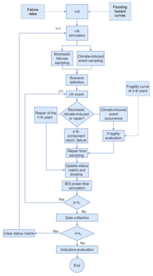
Figure 1.
The flowchart of the simulation framework.
The pseudocode of the simulation framework is as follows:
- (1)
- For to :
- (2)
- i = i + 1
- (2.1)
- For γ = 1 to Γ:
- 2.1.i
- Sample the occurrence times [yy] of the j-th stochastic failure and climate-induced event ( years are neglected, as the longest plant useful life considered (i.e., that of the NPP) is equal to 50 years);
- 2.1.ii
- Sample the flooding level and define the fragility curve , γ = 1, 2,…, Γ, in relation to the sampled flooding level.
- (2.2)
- Sort in increasing order (i.e., a total of events are considered for each scenario).
- (2.3)
- For
- 2.1.iii
- If the j-th event is a stochastic failure event:
- 2.1.iii.1
- The plant fails;
- 2.1.iii.2
- The plant recovery time is sampled.
- 2.1.iv
- If the j-th event is a repair event:
- 2.1.iv.1
- The plant recovers from failure;
- 2.1.iv.2
- A plant failure time is sampled.
- 2.1.v
- If the j-th event is an external event [10]:
- 2.1.v.1
- Sample a random from U [0, 1]:
- 2.1.v.1.1
- If , the γ-th plant fails due to the event and a repair time for each failed plant is sampled.
- 2.1.v.1.2
- If , the γ-th plant withstands the event.
- (2.4)
- The power-flow model described in Section 3.1 is run to calculate the energy import and the energy losses (see Equation (11)) during the 24 h, that are stored in and .
- (2.5)
- j = j + 1 and return to 2.3.i.
- (3)
- Record the number of outages (i.e., energy import events and the internal losses Intl;
- (4)
- Return to 2.
- (5)
- Indicators evaluation:
- (5.1)
- SAIFI is computed as in Equation (1):
- (5.2)
- For the -th climate change projection, the AFP is calculated as the annual import probability that is given by the number of simulations that result in , divided by the total number of simulations:
- (5.3)
- The Zobel resilience metric is computed as:where T is the mean outage duration, i.e., the time between the start of the system failure event and its restoration.
- (5.4)
- For the -th climate change projection, the LEP is given by the ratio between the number of simulations resulting in (i.e., the Italian average value) during the specific year, and the total number of simulations:
- (5.5)
- CVaR is computed with respect to the distribution of energy import :where is the confidence level.
3. The Case Study
We consider an IES composed of different production plants that can be allocated in three possible system layouts, i.e., a standard CS, an IES implementing energy hub (IES-DG) and an IES adding bidirectional energy conversion (IES+P2G). In detail, the CS layout considers large-scale plants of either traditional or renewable energy sources, the IES-DG layout contains multiple medium-size prosumers, referred to as energy hubs (EH) [22], whereas the IES+P2G considers the addition of a storage, in the form of a P2G conversion plant, that converts the excess energy in the grid into natural gas and feeds it into the pipelines. For illustrating purposes, the generic IES considered consists of an NPP (for baseload generation), two CCGT plants (for both baseload and peak regulation), a solar PV field, two WFs, a compression station (to overcome losses in the gas pipes) and a P2G station for energy storage (that can be switched off for simulating the CS layout). The system considered is plotted in Figure 2, adapting it from previous works, such as [23,24]. In particular, we assume that the IES mimics the positioning of a number of realistic plants based in central Italy between Lazio and Campania regions (Figure 3): for the NPP we assume the data of the Garigliano BWR nuclear reactor, CCGT are Napoli-levante and Teverola power plants, WF consists in fleets of Vesta V90 (2000 kW) turbines and solar PVs are fields of 1 kW PV panels with 35° and 180° of tilt and azimuth angles, respectively, summing up to 200 MW (Table 1), as a compromise of the results presented in [25]. In each node, energy can be either injected or absorbed into/from the grid: the six production plants (nodes 1 to 6) and the eight user nodes (nodes 7 to 14) are connected in a ring with nominal voltage of 220 kV, where a radial grid (blue in Figure 2) distributes gas and feeds the gas plants and gas customers. In Table 2 and Table 3, the physical parameters (length, resistance and reactance) of the electric grid connecting the m-th and the n-th nodes corresponding to the production plants, and of the pipes connecting the ϑ-th and φ-th nodes of the pipeline network (length and frictional factor) are listed, respectively. Notice that a virtual additional node (15) is added to the grid (not shown in Figure 1) to account for the “import”, when the IES cannot provide enough energy to customers.
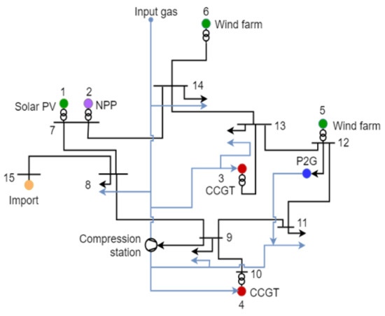
Figure 2.
Sketch of the considered IES.
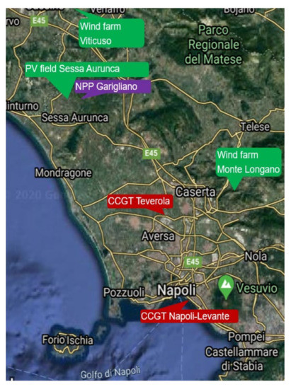
Figure 3.
The locations of the plants considered in the IES of Figure 2.

Table 1.
Characteristics of the production plants.
Table 2.
Power-grid physical parameters.
Table 3.
Pipeline physical parameters.
Without loss of generality, the power demand of user nodes has been set according to a typical power demand profile during July 2018 [26], as shown in Figure 4. This has been taken as a reference demand because it challenges the IES due to the high demand values that must be supplied while complying, at the same time, with the following technical constraints: minimum load for CCGT plants equal to 40% of the nominal power [27], maximum power for the CCGT equal to 110% of nominal power [28] and NPP for baseload only with constant power production at nominal power.
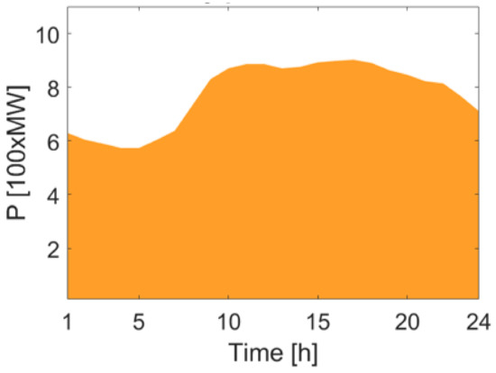
Figure 4.
Power demand for a typical day of July 2018 (TERNA s.p.a.).
The characteristics and models of the EHs that are used in the IES-DG and IES+P2G layouts have been taken from [22]. The EH internal energy demand is satisfied with a small wind turbine and a combined heat and power station (each EH has a total generation capacity of 1200 kW to satisfy its demand and can exchange power with the grid). In our work, this means that EHs can dispatch power to the grid in case of excess of power production to satisfy normal users demand, and the overall power demand of Figure 4 must be discounted by the internal demand and the dispatched power, when the eight EHs, each one connected to one load node, are considered.
3.1. The Simulation of the IES Response
A power-flow model is used to calculate voltage V and phase at each bus of a power system, for a specified load, generator power and voltage condition [24]. This entails defining analytical models for each component of the power system, e.g., electric grid, gas pipeline and energy conversion system. In practice, with reference to our case study, the power flow allows computing Vm and in each m-th electric grid node, the active and reactive power and , respectively, generated/absorbed power in the m-th node and, indirectly, pressure in each -th gas distribution node and volume flow rate in each pipeline connecting the -th and the -th nodes of the gas network [29]. The power-flow model provides, at each iteration τ, the steady state solution of (hereafter indicated as and of F, correspondingly:
where is the variable matrix composed of voltage phase angle vector () at the m-th electric node, voltage magnitude vector (), CCGT power generated (), P2G and gas compressor power demand , ), pressure at the -th pipeline node () and mass flow rate in the -th pipeline edge (); is the system function matrix composed by active and reactive power (, ), pressure (), mass flow rate () and compressor power ().
To simulate the IES of Figure 2 working in nominal conditions (in all the considered layouts of CS, IES-DG and IES+P2G) when the power demand is as in Figure 4 [26], the power-flow model is run 24 times, each one considering the system stationary conditions at each hour of the day (τ = 1, 2, …, 24). From this, the following quantities can be calculated:
- The daily energy exchanged by each m-th node:where (τ) is the active power of the m-th node at the τ-th hour;
- The overall energy supply :
- The overall energy demand :
- The system energy losses (%) , due to distribution losses along cables:
Under normal conditions (i.e., neither stochastic nor climate-induced failures are effecting the operation of the production plants and, therefore, the IES) and when the power demand is as in Figure 4, the energy supplied by each production plant is shown in Figure 5, where the different shades of colors correspond to the energy supplied by each production plant (CCGT, PV, WF and NPP, respectively, in blue, yellow green and red). In all cases, a difference between the demand curve (dashed line) and the supply can be noticed (and quantified with as in Equation (11)). In all cases where , some energy is imported through the virtual node (15) and, in this work, for simplicity, but without loss of generality, the IES is considered failed, because not capable of fulfilling its function of guaranteeing the regional energy independence and security.
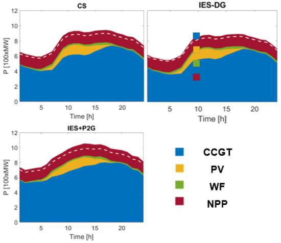
Figure 5.
and for the different layouts (CS, IES-DG, IES+P2G) working in nominal conditions, when the power demand (dashed line) corresponds to Figure 4 (17 July 2018).
We also notice that:
- (1)
- For the IES-DG layout, the difference is smaller than for the CS layout, because the EHs produce (locally) part of the required demanded energy, that is actually discounted to the total demand;
- (2)
- In the IES+P2G layout, the positive balance of EHs in the central hours of the day and the PV power generation allows CCGT plants “to follow” the demand curve more gradually, independently from renewable energy production oscillation, thanks to the P2G. Indeed, the P2G, in case of high renewable generation, stores energy in the form of gas and avoids large-power demand oscillations.
- (3)
- (which increases with the power transmitted by the grid) is the largest for the IES+P2G layout (5.33%), whereas, thanks to local production, are the smallest for the IES-DG layout (3.51%) and the CS layout (4.28%) (vlues compared with Italian grid average of 5.7% in 2018 [26]).
3.2. The IES Reliability Model
The production plants (γ = 1, 2, 3, 4, 5, 6 of Table 1) that compose the IES can fail due to both stochastic and climate-induced failures. Stochastic failures usually originate from fatigue and strain of components [2], and their uncertain failure (or repair) times are, as usual [15], modeled as exponentially distributed:
where is the probability that the γ-th production plant fails (recovers) at time t (i.e., moves from the nominal state k to a failed state (or viceversa)), and and are the failure and repair rates, respectively (see Table 4, where and are given for each γ-th production plant) [30].
Table 4.
Reliability data for system components.
Climate-induced failures are, instead, originated from a natural event that might affect more than one plant at the same time; therefore, climate-induced failures cannot be considered statistically independent (as we assume for the stochastic failures), calling for a different modeling approach. Failures are, indeed, here modeled as “shock” events affecting all plants at the same time that may or may not fail under the shock received, depending on their fragility. For quantitative evaluation, the probability of failure of the γ-th plant due to the δ-th natural event is calculated as:
where is the probability that the γ-th plant fails at time t due to the occurrence of the δ-th event (i.e., the fragility of the γ-th plant to the δ-th event), and is the probability of δ-th event occurrence (e.g., a specific δ-th flooding level occurrence). is calculated using fragility curves that can be obtained by fitting failure databases. In this work, we assume the following fragility curves; for each γ-th power production plant:
- Solar PV panels (γ = 1) are assumed to fail with certainty = 1) when the flooding level exceeds 1 m and to not fail ( = 0) for lower flooding levels, as plotted in Figure 6 (we conservatively assume that 1 m is the height at which electric equipment is mounted on the PV metal structure and this is the equipment that would be damaged by flooding).
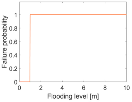 Figure 6. Fragility curve for PV panels.
 - NPP (γ = 2) is assumed to fail with certainty = 1) when flooding level exceeds 5.7 m, and to not fail ( = 0) for lower flooding levels, as plotted in Figure 7 [31].
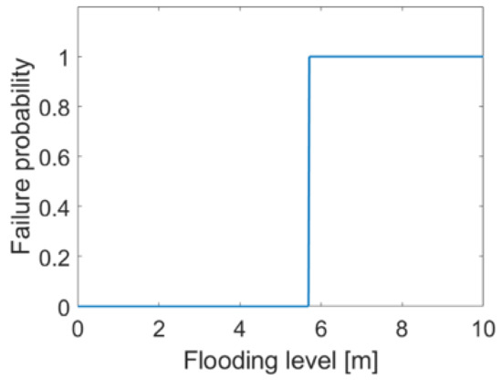 Figure 7. Fragility curve for NPP.
 - CCGT power plants (γ = 3, 4) are assumed to fail with as shown in in Figure 8; different failure probability curves are given for six damage states (negligible, very low, low, medium, relevant and severe) of the concrete walls of CCGT power plants [32]. In this work, the fragility related with the medium damage state is considered (bold line in Figure 7).
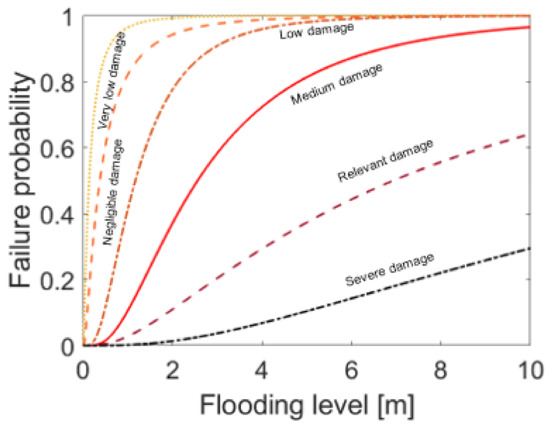 Figure 8. Fragility curves for CCGT.
 - WF (γ = 5, 6) are assumed to fail with certainty (P(t,γ = 5, 6|δ) = 1) when flooding level exceeds 2 m, and to not fail (P(t,γ = 5, 6|δ) = 0) for lower flooding levels, as plotted in Figure 9 (we conservatively assume that 2 m is the maximum flooding level withstood by the transformer connecting the plant to the grid, which is the equipment that would be damaged by the flooding).
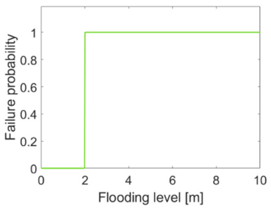 Figure 9. Fragility curve for WF.
Flooding occurrence probability P(δ) can be obtained from the outcomes of TSUMAPS-NEAM (http://www.tsumaps-neam.eu/, accessed on June 2019), an international collaborative project aimed at developing tsunami hazard maps for coastal areas in the North-East Atlantic Mediterranean (NEAM) region. As an example, in Figure 10, we show the P(δ) for a flooding return time of 50 years in a generic site of the NEAM region.
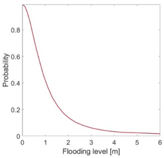
Figure 10.
Probability of flooding level occurrence for a return time of 50 years [http://www.tsumaps-neam.eu (accessed on 19 June 2019)].
It is worth pointing out that, as discussed in [11], flooding can originate from different threats, such as heavy rainfall, storm surges or tsunamis that, as a chain of events, often overlap each other. For simplicity, but without loss of generality, in this work we assume that floods are modeled independently from each other (i.e., each δ-th event is completely resolved before the following one is initiated).
3.3. NaTech Events under Climate Change
The climate-induced failures discussed in Section 3.2 deserve particular care when modeled, due to the variability across space (latitude and longitude) and time (short- or long-time projections). This means working with climate data specific to the IES site (rather than on general worldwide projections) and, also, focusing on specific initiating events (i.e., seismic activity), rather than a multitude of generic sets of natural events. In this work, we tailor the analysis on a specific site (latitude 40° 50′ N, and longitude 14°15′ E, where the IES described in Section 3.1 is located) and consider different time projections (in the (year) 2040, 2070 and 2100) for the flooding hazard curves. As flood-driven failures are strongly related to climate change, which induces stronger and more frequent events [9], we model the flooding severity to increase with the sea level rise that is ultimately dependent on the temperature rise [33]. In practice, the 8.5 RCP sea-level increase projections = [0, 0.2003, 0.3889, 0.5970] for = [2020 2040 2070 2100] are used to fit Equation (15) (corresponding to the flooding hazard curves of Figure 11), starting from the baseline curve of Equation (14) proposed by [14] as the probability of flood level in 2020:
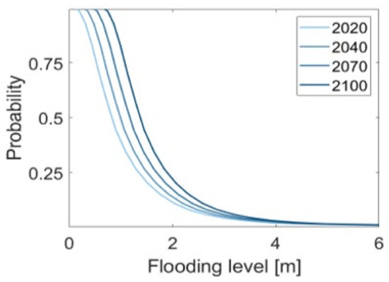
Figure 11.
Probability of flooding level occurrence for a return time of 50 years [http://www.tsumaps-neam.eu (accessed on 19 June 2019)] for each climate change projection (2020, 2040, 2070 and 2100).
It is worth noticing that between 2020 and 2100, the flooding occurrence probability almost doubles (at fixed severity) and that the most frequent events consistently increase in severity, endangering the IES integrity, as long as the climate changes.
4. Results
The framework presented in Section 2 has been applied for the analysis of the IES described in Section 3. The following analysis considers the IES+P2G layout (i.e., the most complete layout among CS, IES-DG and IES+P2G) subject to stochastic and climate-induced failures under a climate change projection over the horizon to 2100 (i.e., the most conservative and threatening scenario), to analyze which failure mechanism (stochastic or climate-induced) plays the major role.
We consider = 10,000 alternative stochastic scenarios, which are run on MATLAB with a Dell XPS: Intel Core i7-8550U CPU @1.8 Ghz and 8 GB RAM.
In Figure 12, the SAIFI boxes are shown for comparing the results when stochastic, climate-induced failures and (their) combined effects are considered. It is worth mentioning that, as already stated, state-of-the art framework of analysis entails accounting only for stochastic failures. With this proposed approach, instead, it can be quantified the joint effect of the large number of import events due to the stochastic failures (due to the large failure rate of the CCGT), and the lower number of climate-induced failures (due to low-frequency and high-severity events).
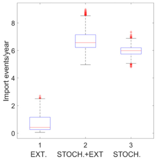
Figure 12.
SAIFI.
The R and CVaR (for β = 90%, 95% and 99% confidence levels) are provided in Table 5, and again for comparing the results of stochastic, climate-induced failures and (their) combined effects; climate-induced failures are shown to have the largest impact on . As a matter of fact, all the CVaR values, when considering climate-induced failures, are larger than those of stochastic failures. AFP and LEP, shown in Figure 13 and Figure 14, respectively, are close to 1 when stochastic (only) and (both) stochastic and climate-induced failures are considered, due to the large share of power produced by the CCGT; any stochastic failure of any single plant may lead to an energy import, whereas climate-induced failures, which more likely affect small power production plants, can be easily covered by the remaining operating plants.
Table 5.
CVaR(β) and R.
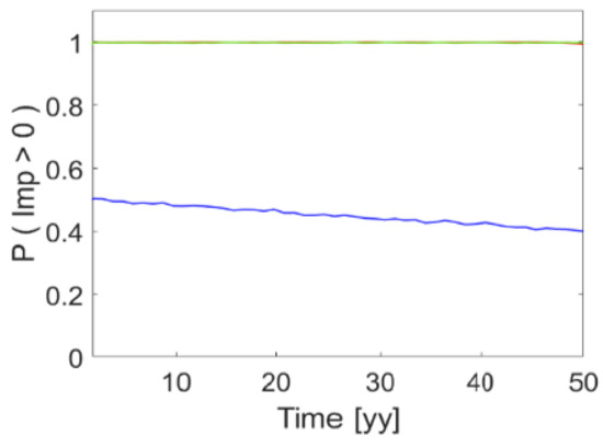
Figure 13.
AFP.
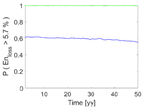
Figure 14.
LEP.
The effect of climate-induced failures on the performance of the IES+P2G layout is noticeable and quantifiable, with the proposed modeling and analysis framework: for example, the resilience of the system due to climate-induced shock events (blue line in Figure 15) demonstrates less resourcefulness for recovering from natural hazards events with respect to only stochastic failures (red line). This is due to the fact that, in general terms, low severity (high frequency) climatic events affect PV and WF (characterized by low production capacity and long repair times), whereas the frequent stochastic failures that affect the CCGT plant are more promptly recovered, as they are likely to occur and maintenance readiness is expected to recover the systems.
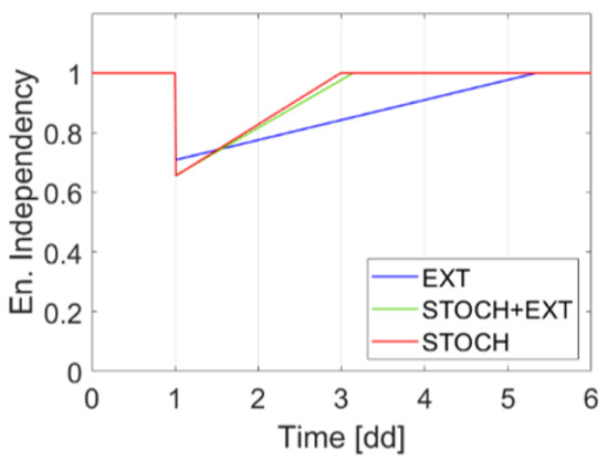
Figure 15.
Resilience.
In conclusion, the analysis of the case study here provided shows how the proposed framework can be operationalized to jointly consider and model stochastic and climate-induced failures. The outcomes obtained warn against the fact that neglecting the contribution of the latter could expose an IES to additional risks: the identification and quantification of these by the proposed framework can also inform the proper planning and designing IES, and support decision making and policy-making when adaptation to climate change is to be duly considered.
5. Conclusions
In this work, we have presented a modeling framework for the analysis of IES that considers both stochastic failures and climate-induced events. The framework, which is operationalized with a double-loop Montecarlo simulation, has been applied to a typical IES+P2G layout of power production exposed to flooding scenarios, to evaluate a pool of representative indicators, such as SAIFI, AFP, R index, LEP and CVaR. Results suggest that power systems withstand better climate change when energy production systems are integrated, as in the IES+P2G layout. This is because, as expected, the failures on certain plants can be mitigated by the capability offered by other plants and EHs connected to the network. It is worth mentioning that, if the IES+P2G suffers (from the resilience point-of-view) the P2G electric demand that makes the system more vulnerable to climate-induced failure events, it is the preferred solution when the infrastructure is suffering from a gas shortage. As a last remark, it is important to point out that the presented results, due to the large uncertainty that affects the climate change models, need a rigorous uncertainty quantification and analysis to allow for decision making with confidence. Future work will, therefore, focus on the development of uncertainty quantification approaches that can capitalize the Monte Carlo simulations results that the framework presented here can provide.
Author Contributions
Conceptualization, F.D.M. and E.Z.; methodology, F.D.M. and E.Z.; formal analysis, P.T.; investigation, P.T. and F.D.M.; writing—original draft preparation, P.T.; writing—review and editing, F.D.M. and E.Z.; supervision, F.D.M. and E.Z.; funding acquisition, F.D.M. All authors have read and agreed to the published version of the manuscript.
Funding
This research was funded by MIUR—Italian Ministry for Scientific Research under the PRIN 2017 program (grant 2017CEYPS8) for the research titled “Assessment of Cascading Events triggered by the Interaction of Natural Hazards and Technological Scenarios involving the release of Hazardous Substances”.
Institutional Review Board Statement
Not applicable.
Informed Consent Statement
Not applicable.
Conflicts of Interest
The authors declare no conflict of interest.
| List of Symbols | |
| Confidence level of CVar | |
| Number of plants within the IES | |
| Index of the plant within the IES | |
| Pressure variation | |
| Compressor power variation | |
| Active power variation | |
| Reactive power variation | |
| Mass flow-rate function | |
| Voltage phase angle at the -th electric node | |
| Failure rate of -th plant | |
| Pressure at the -th pipeline node | |
| Power-flow iteration | |
| Energy demand | |
| Energy import during the 24 h | |
| Energy losses during the 24 h | |
| Daily energy exchanged by -th node | |
| Overall energy supply | |
| System function matrix | |
| Fragility curve of -th plant | |
| Future year | |
| Sea level increase projected in | |
| Internal losses | |
| Index for the Monte Carlo simulation | |
| Index for the events that occur during the simulation | |
| Number of outages | |
| Number of events considered for each scenario | |
| Number of Monte Carlo simulation | |
| Probability of failure of the -th plant due to the -th climate induced natural event | |
| Probability that the -th production plant fails (recover) at time (i.e., moves from the nominal state to a failed state (or viceversa)) due to stochastic events | |
| Active power | |
| Probability of -th event occurrence | |
| Probability of flood level in | |
| Probability that the -th plant fails at time due to the occurrence of the -th event | |
| Gas compressor power demand | |
| CCGT power generated | |
| P2G power demand | |
| Pressure in the -th gas distribution node | |
| Volume flow rate in each pipeline connecting the -th and the -th nodes of the gas network | |
| Reactive power | |
| Zobel resilience metric | |
| Repair rate of -th plant | |
| Mean outage duration | |
| Occurrence time of the j-th stochastic failure or climate-induced event | |
| Random number sampled from an uniform distribution | |
| Voltage in -th electric grid node | |
| Voltage magnitude vector | |
| Variable matrix | |
| List of Acronyms | |
| AFP | Annual Failure Probability |
| CCF | Common Cause Failure |
| CCGT | Combined Cycle Gas Turbine Plant |
| CS | Centralized System |
| CVaR | Conditional Value at Risk |
| EH | Energy Hub |
| IES | Integrated Energy System |
| IES+P2G | IES with bidirectional energy conversion enabled by power-to-gas facilities (P2G) |
| IES-DG | IES with Distributed Generation |
| LEP | Loss Exceedance Probability |
| NaTech | Natural Technological |
| NEAM | North-East Atlantic Mediterranean |
| NPP | Nuclear Power Plant |
| P2G | Power-to-Gas station |
| PV | Solar Photovoltaic |
| RCP | Representative Concentration Pathway |
| SAIFI | System Average Interruption Frequency Index |
| WF | Wind Farm |
References
- Yodo, N.; Wang, P.; Rafi, M. Enabling Resilience of Complex Engineered Systems Using Control Theory. IEEE Trans. Reliab. 2017, 67, 53–65. [Google Scholar] [CrossRef]
- Zio, E. The Montecarlo Simulation Method for System Reliability and Risk Analysis; Springer: Berlin/Heidelberg, Germany, 2012. [Google Scholar]
- Teh, J.; Lai, C.-M. Risk-Based Management of Transmission Lines Enhanced with the Dynamic Thermal Rating System. IEEE Access 2019, 7, 76562–76572. [Google Scholar] [CrossRef]
- Sahlin, U.; Di Maio, F.; Vagnoli, M.; Zio, E. Evaluating the impact of climate change on the risk assessment of Nuclear Power Plants. In Safety and Reliability of Complex Engineered Systems; CRC Press: Boca Raton, FL, USA, 2015; pp. 2613–2621. [Google Scholar]
- Savelsberg, J.; Schillinger, M.; Schlecht, I.; Weigt, H. The impact of climate change on Swiss hydropower. Sustainability 2018, 10, 2541. [Google Scholar] [CrossRef]
- Mitra, B.K.; Sharma, D.; Zhou, X.; Dasgupta, R. Assessment of the impacts of spatial water resource variability on energy planning in the ganges river basin under climate change scenarios. Sustainability 2021, 13, 7273. [Google Scholar] [CrossRef]
- Borghetti, A.; Cozzani, V.; Mazzetti, C.; Nucci, C.; Paolone, M.; Renni, E. Monte Carlo based lightning risk assessment in oil plant tank farms. In Proceedings of the 2010 30th International Conference on Lightning Protection (ICLP), Cagliari, Italy, 13–17 September 2010; pp. 1–7. [Google Scholar]
- Olivar, O.J.R.; Mayorga, S.Z.; Giraldo, F.M.; Sanchez-Silva, M.; Salzano, E. «The effect of Extreme Winds on Industrial Equipment. Chem. Eng. Trans. 2018, 67, 871–876. [Google Scholar]
- Collins, M.; Knutti, R.; Arblaster, J.; Dufresne, J.L.; Fichefet, T.; Friedlingstein, P.; Gao, X.; Gutowski, W.J.; Johns, T.; Krinner, G.; et al. Long-term Climate Change: Projections, Commitments and Irreversibility. In Climate Change 2013-The Physical Science Basis: Contribution of Working Group I to the Fifth Assessment Report of the Intergovernmental Panel on Climate Change; Cambridge University Press: Cambridge, UK, 2013. [Google Scholar]
- Zio, E.; Ferrario, E. A framework for the system-of-systems analysis of the risk for a safety-critical plant exposed to external events. Reliab. Eng. Syst. Saf. 2013, 114, 114–125. [Google Scholar] [CrossRef][Green Version]
- Iervolino, I.; Baltzopoulos, G.; Chioccarelli, E.; Suzuki, A. Seismic actions on structures in the near-source region of the 2016 central Italy sequence. Bull. Earthq. Eng. 2017, 17, 5429–5447. [Google Scholar] [CrossRef]
- Shen, Y.; Morsy, M.M.; Huxley, C.; Tahvildari, N.; Goodall, J.L. Flood risk assessment and increased resilience for coastal urban watersheds under the combined impact of storm tide and heavy rainfall. J. Hydrol. 2019, 579, 124159. [Google Scholar] [CrossRef]
- Duan, J.; van Kooten, G.C.; Liu, X. Renewable electricity grids, battery storage and missing money. Resour. Conserv. Recycl. 2020, 161, 105001. [Google Scholar] [CrossRef]
- Pitilakis, K.; Argyroudis, S.; Fotopoulou, S.; Karafagka, S.; Kakderi, K.; Selva, J. Application of stress test for port infrastructures against natural hazards. The case of Thessaloniki port in Greece. Reliab. Eng. Syst. Saf. 2018, 184, 240–257. [Google Scholar] [CrossRef]
- Riahi, K.; Rao, S.; Krey, V.; Cho, C.; Chirkov, V.; Fischer, G.; Kindermann, G.E.; Nakicenovic, N.; Rafaj, P. RCP 8.5—A scenario of comparatively high greenhouse gas emissions. Clim. Chang. 2011, 109, 33–57. [Google Scholar] [CrossRef]
- Kopp, R.E.; Horton, R.M.; Little, C.M.; Mitrovica, J.X.; Oppenheimer, M.; Rasmussen, D.J.; Strauss, B.H.; Tebaldi, C. Probabilistic 21st and 22nd century sea-level projections at a global network of tide-gauges sites. Earth’s Future 2014, 2, 363–406. [Google Scholar] [CrossRef]
- Li, G.; Bie, Z.; Kou, Y.; Jiang, J.; Bettinelli, M. Reliability evaluation of integrated energy systems based on smart agent communication. Appl. Energy 2016, 167, 397–406. [Google Scholar] [CrossRef]
- Korkali, M.; Veneman, J.G.; Tivnan, B.F.; Bagrow, J.P.; Hines, P.D. Reducing Cascading Failure Risk by Increasing Infrastructure Network Interdependence. Sci. Rep. 2017, 7, 44499. [Google Scholar] [CrossRef]
- Chang, S.E.; Shinozuka, M. Measuring Improvements in the Disaster Resilience of Communities. Earthq. Spectra 2004, 20, 739–755. [Google Scholar] [CrossRef]
- Pant, R.; Barker, K.; Zobel, C.W. Static and dynamic metrics of economic resilience for interdependent infrastructure and industry sectors. Reliab. Eng. Syst. Saf. 2014, 125, 92–102. [Google Scholar] [CrossRef]
- Dixit, V.; Verma, P.; Tiwari, M.K. Assessment of pre and post-disaster supply chain resilience based on network structural parameters with CVaR as a risk measure. Int. J. Prod. Econ. 2020, 227, 107655. [Google Scholar] [CrossRef]
- Pazouki, S.; Haghifam, M.R. Optimal planning and scheduling of energy hub in presence of energy wind, storage and de-mand response under uncertainty. Electr. Power Energy Syst. 2016, 80, 219–239. [Google Scholar] [CrossRef]
- Su, H.; Chi, L.; Zio, E.; Li, Z.; Fan, L.; Yang, Z.; Liu, Z.; Zhang, J. A systematic data-driven Supply-Demand Management method for smart Inte-grated Energy Systems. Energy 2019, 235, 121416. [Google Scholar] [CrossRef]
- Zeng, Q.; Fang, J.; Li, J.; Chen, Z. Steady-state analysis of the integrated natural gas and electric power system with bi-directional energy conversion. Appl. Energy 2016, 184, 1483–1492. [Google Scholar] [CrossRef]
- Hailu, G.; Fung, A.S. Optimum Tilt Angle and Orientation of Photovoltaic Thermal System for Application in Greater Toronto Area, Canada. Sustainability 2019, 11, 6443. [Google Scholar] [CrossRef]
- TERNA s.p.a.e. Gruppo. Dati Statistici Sull’energia Elettrica in Italia. 2018. Available online: www.terna.it (accessed on 19 June 2019).
- Sala, L.; Calzolari, F.; Traverso, R.; Tuscano, S.; Bruschi, G.; Gatti, R. La sfida Tecnologica di Ansaldo Energia per la Gestione Flessibile dei Cicli Combinati, Ansaldo Report. 2018. Available online: https://www.verticale.net/la-sfida-tecnologica-di-ansaldo-energia-4414 (accessed on 19 June 2019).
- Saravanamuttoo, H.I.; Rogers, G.F.C.; Cohen, H. Gas Turbine Theory; Pearson Education: London, UK, 2008. [Google Scholar]
- di Maio, F.; Morelli, S.; Zio, E. A Simulation-Based Framework for the Adequacy Assessment of Integrated Energy Systems Exposed to Climate Change. In Handbook of Smart Energy Systems; Fathi, M., Zio, E., Pardalo, P.M., Eds.; Springer Nature: Basingstoke, UK, 2022. [Google Scholar]
- Roos, F.; Lindah, S. Distribution System Component Failure Rates and Repair Times—An Overview. In Nordic Distribution and Asset Management Conference; Lund University: Lund, Sweden, 2004. [Google Scholar]
- Nuclear Regulatory Commission. U.S. Severe Accident Risks: An Assessment for Five U.S: Nuclear Power Plants; NUREG-1150; Nuclear Regulatory Commission: Rockville, MD, USA, 1990; Volume 1.
- Sabouhi, H.; Abbaspour, A.; Fotuhi-Firuzabad, M.; Dehghanian, P. Reliability modeling and availability analysis of combined cycle power plants. Int. J. Electr. Power Energy Syst. 2016, 79, 108–119. [Google Scholar] [CrossRef]
- Le Cozannet, G.; Bulteau, T.; Castelle, B.; Ranasinghe, R.; Wöppelmann, G.; Rohmer, J.; Bernon, N.; Idier, D.; Louisor, J.; Salas-Y-Mélia, D. Quantifying uncertainties of sandy shoreline change projections as sea level rises. Sci. Rep. 2019, 9, 42. [Google Scholar] [CrossRef] [PubMed]


Publisher’s Note: MDPI stays neutral with regard to jurisdictional claims in published maps and institutional affiliations. |
© 2022 by the authors. Licensee MDPI, Basel, Switzerland. This article is an open access article distributed under the terms and conditions of the Creative Commons Attribution (CC BY) license (https://creativecommons.org/licenses/by/4.0/).