Abstract
The environmental pollution in the Beijing–Tianjin–Hebei region is of serious concern, and the environmental impact of dispersing Beijing’s non-capital functions and promoting industrial transfer in an orderly manner cannot be ignored. Based on the spatial panel model, the environmental impact effect of industrial transfer on pollutants was analyzed using the panel data of 13 regions in Beijing–Tianjin–Hebei Province from 2004 to 2018, and the total effect EKC curve was decomposed into direct and indirect effect EKC curves. The results showed the following: (1) The total effect of industrial transfer had a restraining effect on the emission intensity of three types of industrial pollutants. The direct and indirect effects of industrial transfer can significantly inhibit the emission intensity of industrial wastewater, whereas only the indirect effect of industrial transfer can reduce the emission intensity of industrial SO2 and SO2 in the region. (2) The EKC of the indirect and total effects of industrial SO2, wastewater, and dust was an inverted u-shape, and the EKC of the direct effect of industrial wastewater was a positive u-shape. Except for industrial dust, industrial SO2 and wastewater have exceeded the inflection point. With the development of per capita GDP, the emission intensity of industrial pollutants is showing a downward trend. Therefore, the Beijing–Tianjin–Hebei region should gradually transfer pollution-intensive industries, jointly protect the environment, prevent and control pollution, adjust the industrial structure, optimize the industrial layout, promote the development of a circular economy, and promote high-quality development.
1. Introduction
The economy and the environment are the two major themes of human social development. General Secretary Xi Jinping has pointed out that protecting the ecological environment is to protect productivity, and improving the ecological environment is to develop productivity. The air pollution in the Beijing–Tianjin–Hebei region is significant. According to the National Urban Air Quality Report in May 2021, there are 12 cities with air pollution transmission channels in Beijing–Tianjin–Hebei, accounting for 60% of the 20 cities with relatively poor air quality in China. Resolving Beijing’s non-capital function, promoting orderly industrial transfer, optimizing the industrial spatial layout, upgrading traditional industries, and eliminating backward production capacity are necessary choices for realizing the coordinated development of the economy and environment in the Beijing–Tianjin–Hebei region.
Thus, exploring the relationship between industrial transfer and the environment can provide new ideas for improving environmental quality. Based on this, this paper used a spatial econometric model to analyze the direct effect, indirect effect, and total effect of industrial transfer on the environment. In addition, this paper also used the EKC curve as an effective tool to deeply analyze economic growth and environmental problems [1]. This paper incorporated the industrial transfer index into the EKC analysis framework to analyze the environmental impact of industrial transfer, to provide theoretical support and suggestions for the coordinated green development of the Beijing–Tianjin–Hebei region.
This paper makes the following three marginal contributions: (1) This paper explored the relationship between industrial transfer and industrial sulfur dioxide, industrial wastewater, and industrial soot, not only to explore the impact of industrial transfer on environmental quality, but also to provide a more detailed reference for policy formulation. (2) The spatial econometric model was used to explore the spatial direct effect, spatial spillover effect, and spatial total effect between industrial transfer and environmental quality. Compared with ordinary panel regression, the empirical analysis of this paper considered the spatial correlation between variables. (3) Whether there is an EKC curve in the direct effect, indirect effect, and total effect of industrial sulfur dioxide, industrial wastewater, and industrial soot was discussed, improving the conclusions of the existing literature.
The content of this paper is arranged as follows: the second part is literature review, the third part is model design and data interpretation, the fourth part is real evidence analysis, the fifth part is conclusion, and the sixth part is recommendations. The specific research framework is shown in Figure 1.
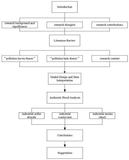
Figure 1.
Research framework.
2. Literature Review
The environmental effect of industrial transfer is a research hotspot in related fields. Many academic circles have discussed whether the ecological impact of industrial transfer is negative or positive. Some scholars suggest the former and others the latter, thus forming the “pollution haven theory” and “pollution halo theory” [2].
People in developed countries or regions tend to have higher environmental demands [1]. Governments may adopt stricter environmental regulations, while less developed countries or regions consider economic development as the primary goal and adopt looser environmental rules. A more open environmental code means lower ecological costs, and enterprises with high energy consumption and high pollution that are chasing profits will gradually shift to less developed regions. At the same time, due to the aggregation of pollution-intensive industries, the natural environment of the areas of industrial transfer will also come under increasing pressure, which is the so-called “pollution haven theory” [3,4]. Around this theory, scholars at home and abroad have undertaken much empirical analysis. Sun et al. took Beijing as the research object [4]. They empirically analyzed the inter-regional transfer process of industries in combination with the fact that Beijing’s “non-capital function” industries were being liberated outwards. Akbostanci et al. pointed out that the environmental concerns of developed economies led them to formulate strict environmental regulations, which increased the production cost of domestic polluting industries [5]. Akbostanci et al. [5] believe pollution-intensive industries have shifted from developed to developing countries. Li thought that the pioneering development of the secondary sector reduced the carbon emissions of all provinces in China [6]. Silva and Zhu found that with free and open trade, poorer countries become pollution havens for emissions trading [7].
The research framework suggests that the process of transferring excess capacity from developed to less developed countries or regions is accompanied by the transfer of sustainable management concepts [8], advanced management models [9,10], and green innovation technologies (Figure 2). The transfer of excess capacity can effectively promote innovation management, reform management modes, and innovative green development technology in underdeveloped areas, and then promote the industrial carrying capacity to improve the environment. Wang et al. [8] found through empirical tests that the transfer of pollution-intensive industries in Beijing has had a typical pollution halo effect. Mert and Caglar argue that an increase in foreign direct investment leads to a decline in the growth rate of emissions, which supports the asymmetric pollution halo hypothesis [11]. Kisswani and Zaitouni studied the impact of foreign direct investment on pollution in Malaysia and Singapore from 1971 to 2014. The results supported the pollution halo hypothesis in Malaysia and Singapore [12].
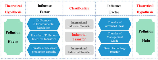
Figure 2.
Analysis of industrial transfer and environmental impact mechanisms.
As shown in Figure 2, both international and interregional industrial transfers have two effects. On the one hand, due to differences in environmental regulations, the high energy-consuming and high-polluting production capacity of developed countries or regions are transferred to less developed countries or regions, place pressure on the local environment. On the other hand, the industrial transfer also brings sustainable development concepts and business model innovation to the industrial carrier to a certain extent, and promotes local enterprises to carry out green technological innovation, thus improving the local environment. Different regions or development stages in the same region have different attitudes towards industrial transfer. Whether industrial transfer will aggravate local environmental pollution or vice versa, and whether the ecological effect of the industrial transfer will be positive or negative, needs to be verified by further empirical research [13].
The academic community has not formed a unified understanding of the comprehensive impact of human beings on the environment [14]. There are two main views on this. The first view is that there is an inverted U-shaped relationship between economic growth and the environment. That is, the environment deteriorates first and then improves with economic growth. The second view is that the inverted U-shaped relationship between economic growth and the environment is related to many factors [15,16,17]. In the EKC (Environment Kuznets Curve) analysis framework, a specific econometric analysis method is generally used [18,19], the dependent variable is the environmental index, and the independent variables include an index representing economic growth and other control variables [20,21,22,23,24,25]. Few studies have introduced industrial transfer into the EKC analysis framework. Liu et al. constructed the industrial transfer index. They used the time series data of the Beijing–Tianjin–Hebei region to analyze the impact of industrial transfer on the economic environment using the traditional econometric model [26]. However, this study did not consider the spatial dependence of industrial transfer. Only the environmental impact effect (direct effect) of industrial transfer in the region was considered, while the environmental impact effect (indirect effect) of industrial transfer in neighboring areas was ignored. Many works on spatial measurement have considered that economic variables often have significant spatial dependence [27]. In addition, most of the EKC empirical analysis literature based on spatial econometric methods discusses the EKC curve based on the estimation results of model coefficients, which is inaccurate [28,29]. Given this, this study introduced industrial transfer into the EKC analysis framework, using a spatial panel data model to analyze the effect of industrial transfer on industrial sulfur dioxide, wastewater, and soot.
3. Model Design and Data Description
3.1. Model Design
3.1.1. Spatial Panel Data Model
The EKC analysis framework based on the non-spatial model ignores the spatial spillover effects of indicators such as pollutant emissions, economic growth, and industrial transfer, which leads to errors in the simulation of economic growth and environmental pollution trends. This paper used the spatial econometric model to reflect the spatial spillover effects of environmental pollution, economic growth, and industrial transfer [30] as an analytical tool. According to the spatial econometric model, the following EKC panel model of the spatial measurement of environmental pollution caused by industrial transfer was established:
In the model, LnPOLit represents environmental pollution, which is jointly represented by three indicators: industrial sulfur dioxide emission intensity, industrial wastewater emission intensity, and industrial smoke (powder) dust emission intensity. is the constant term. is the coefficient of the spatial lag term of the explained variable LnPOLit. W is the spatial weight matrix. LnTRANit is the industrial transfer index. LnControlit is the explanatory variable, including per capita GDP and its quadratic term, total population, proportion of secondary industry, FDI, R&D investment, and the comprehensive utilization rate of industrial solids. is the coefficient column vector of the explanatory variable, is the coefficient column vector of the spatial lag term of the explanatory variable, and are the individual effect and the period effect, respectively, is the random disturbance term of the model (1).
3.1.2. Measurement Method of Three Effects and EKC Curve Decomposition
The standard EKC curve ignores the indirect effect. In contrast, the total effect EKC curve based on the spatial model accurately describes the environmental quality and economic growth. The total effect EKC curve is decomposed into the direct effect EKC curve and indirect effect EKC curve, which can explain the relationship between the environment and economy and its development trend in detail based on the two aspects of the direct effect and indirect effect. However, the total effect, direct effect, and indirect effect cannot be directly speculated by the regression coefficient of the spatial model. It can only be measured by computer simulation based on partial differential theory and tested for significance [30]. According to the measurement results, GDP’s direct, indirect, and total effect were obtained. Combined with the statistical test results, the total effect EKC curve could be decomposed into a direct effect EKC curve and an indirect effect EKC curve.
For the significance test of the three effects, it was impossible to directly calculate whether the three effects of the variables were significant from the coefficients estimated by the spatial model or its T statistics. At the same time, it was not possible to directly derive the significance test statistics of the three effects from the variance and covariance matrix of the model, such as through calculating the T value of the model coefficients. However, we could simulate the three effects based on the variance–covariance matrix obtained by maximum likelihood estimation to analyze the distribution of the three effects. Finally, we used the mean T-test to study the significance of different effects.
3.2. Indicators and Data Description
The core explanatory variable of this paper was the industrial transfer index (ITI, Industrial Transfer Index), which is mainly manifested in the spatial and temporal distribution changes of industrial activities between regions. It can usually be measured by methods such as industrial share, location entropy, industrial gradient index, and deviation-share analysis, or the impact of external events. The index data that can represent the industrial transfer index usually include three types of indicators: concentration, fixed assets, and industrial output value. For example, Wang et al. used a multi-regional input–output model to measure industrial transfer in 30 provinces in China and to compare industrial transfer and carbon transfer paths [31]. Feng et al. [32] pointed out that the deviation share method can make up for the shortcomings of the share index method and the input–output table method. This has been a popular method in recent years. The deviation share method can be used as one of the main measurement methods for future industrial transfer. The industrial output value index is widely used. Based on the added value of the secondary industry and the shift–share analysis method commonly used in academia, this paper constructed the industrial transfer index. The design ideas were as follows:
In the above equation, is the industrial transfer index of region in period , and represent the value added of the secondary industry of region in period and , respectively, and represent the value added of the secondary industry of all regions in period and , respectively; represents the change rate of the value added of the secondary industry in region in the year relative to the year, represents the change rate of the value added of the secondary industry in all regions in the year relative to the t year, and the difference between the two represents the net change rate of the scale of the secondary industry in region ; that is, the industrial transfer index. When , region i is the industry transfer receiver in period . Otherwise, it is the industry transfer exporter.
Different definitions of environmental quality indicators are used in academic circles [33]. According to the corresponding References [34,35], we refer to the “three wastes” emissions; the use of industrial sulfur dioxide emission intensity, industrial wastewater emission intensity, and industrial smoke (powder) dust emission intensity as dependent variables. In addition, combined with the specific circumstances of the 13 Beijing–Tianjin–Hebei regions and reference to relevant literature [36,37], we constructed six control variables from the four dimensions of scale, structure, technology, and trade (Table 1).

Table 1.
Variable selection and definition.
Taking the data of 13 regions in Beijing, Tianjin, and Hebei from 2004 to 2018 as research samples, the data of industrial sulfur dioxide emissions, industrial wastewater emissions, industrial smoke (powder) dust emissions, the comprehensive utilization rate of industrial solid waste, R&D investment, the secondary industry output value, and FDI were from the 2004–2019 “China City Statistical Yearbook”. Total population, per capita GDP, and proportion of secondary industry were from the “China Statistical Yearbook”. Both statistical yearbooks are published by China Statistical Publishing House, which is the only professional publishing house in the field of statistics in the country. The variables in the model are in the form of the natural logarithm to overcome the bias caused by heteroscedasticity. For any undisclosed or missing data in the research sample, trend estimation or the interpolation method were used to fill it in. The descriptive statistics of the variables are shown in Table 2. There were large regional differences between industrial transfer and industrial pollutant emissions in the Beijing–Tianjin–Hebei region from 2004 to 2018. The logarithmic mean of industrial wastewater discharge in 13 regions of Beijing–Tianjin–Hebei was 8.984, and the standard deviation was 0.765. The logarithmic mean of industrial sulfur dioxide emissions was 11.091, and the standard deviation was 0.964. The logarithmic mean value of industrial smoke (powder) dust was 10.563, and the standard deviation was 0.998. The logarithmic mean of industrial transfer was 0.483, and the standard deviation was 0.181. This reflects that the fluctuation in industrial pollutant emissions is large because it is sensitive to macro policy control, R&D investment, foreign direct investment, and other external factors.
Table 2.
Variables Descriptive Statistics.
3.3. Unit Root Test for Panel Data
To avoid the pseudo-regression phenomenon and enhance the reliability of the research conclusions, we conducted a stationarity test on the research data. The panel unit root test methods included the LLC test, Breitung test, IPS test, ADF-Fisher test, PP-Fisher test, etc. We adopted the LLC, IPS, ADF-Fisher, and PP-Fisher four panel unit root test methods. The original sequence of variables and the first-order difference sequence were tested for unit root, and the test results are shown in Table 3. In Table 3, although the individual study variables (Ln(S), Ln(POP), Ln(IND), Ln(PGDP), and Ln2(PGDP)) were accepted under the LLC test form to reject the null hypothesis that there is a unit root, the results of the other three, IPS, ADF-Fisher and PP-Fisher, showed that no matter the original value or the first-order difference sequence, the test statistic rejects the null hypothesis at the 1% level, so there is no unit root. Therefore, the original value sequence and the first-order difference sequence were both stationary and single integral sequences.
Table 3.
Unit root test results of panel data.
3.4. Correlation Test
Table 4 lists the correlation of each study variable and provides the Pearson correlation coefficient of the study variable. According to the correlation coefficient matrix of variables in Table 2, the correlation coefficients between industrial transfer and industrial sulfur dioxide emission intensity, industrial wastewater emission intensity, and industrial smoke (powder) dust emission intensity were −0.25 (p < 0.01) and −0.20 (p < 0.01), respectively, and −0.15 (p < 0.01), indicating that there was a significant negative correlation between industrial transfer and environmental pollution. In addition, most of the correlation coefficient values between the explanatory variables were less than 0.60, and their eigenvalues were not zero. The results of the correlation test showed that it conforms to the research hypothesis and conclusion, which further proves the robustness of the research in this paper.
Table 4.
Correlation coefficient matrix.
3.5. Cross-Sectional Dependence Tests
We used Eviews 11 for the cross-sectional dependence tests. The hypothesis of the tests is: no cross-section dependence (correlation), and the test results are shown in the following table (Table 5). The results show that the variables we used have a serious cross-sectional dependence (p = 0.000). When the real model contains cross-sectional dependence caused by factors, ignoring this cross-sectional dependence generally makes the parameter estimation inconsistent. For this problem, we use the spatial econometric model which can be a good solution. Elhorst et al. pointed out that in the real world, especially when encountering spatial data problems, independent observations are not ubiquitous in real life. In this regard [38], Elhorst et al. proposed that panel data estimation can be performed through spatial econometric models. So, we use spatial econometric model to estimate [38].
Table 5.
Cross-sectional dependence tests.
3.6. Homogeneity Test
The premise of homogeneity test is that the total variance of different variables is equal, so the homogeneity test of variance is carried out. Proposing the null hypothesis: there is no significant difference in the variance of different variables. Using SPSS 16.0 to test the homogeneity of variance, the specific test results are shown in Table 6.
Table 6.
The results homogeneity tests.
It can be seen from Table 6 that the significance level of all variables is much greater than 0.05, indicating that the null hypothesis cannot be rejected, that is, the homogeneity of variance hypothesis is satisfied.
4. Authentic Proof Analysis
In this part, industrial transfer was introduced into the EKC analysis framework, and the spatial panel data model was used to analyze the influence and effect of industrial transfer on industrial sulfur dioxide, industrial wastewater, and industrial smoke (dust), as well as the EKC relationship between economic development and three types of pollutants. In the last part of the empirical study, the robustness check was also carried out.
4.1. Effect of Industrial Transfer on Industrial Sulfur Dioxide Emission Intensity
4.1.1. Influence of Industrial Transfer on Industrial Sulfur Dioxide
The introduction of the square term in the independent variable will lead to the problem of collinearity and affect the estimation effect of the coefficient. Therefore, when analyzing the impact of industrial transfer and other control variables on pollutants, the square term is not considered except when exploring the nonlinear relationship between economic development and pollutant emissions.
Firstly, the spatial weight matrix based on finite distance was selected for analysis, and the robustness analysis was carried out by using a 0–1 matrix and latitude–longitude spatial matrix. Secondly, after screening, the spatial Dubin individual fixed effect model was used to analyze the impact of the industrial transfer on industrial sulfur dioxide emission intensity. Due to spatial autocorrelation, the model coefficients could not fully reflect the full effect of industrial transfer. It was necessary to measure the direct, indirect, and total effects of industrial transfer and analyze the impact of the industrial transfer on the environment according to the three marks and significance test results.
Table 7 shows that the direct effect of the industrial transfer was not significant; the indirect effect of the industrial transfer was −1.161, which was significant at the level of 1%, which means that when other variables remain unchanged, every 1% increase in industrial undertaking in neighboring regions will result in a 1.16% reduction in industrial sulfur dioxide emissions in the region. It should be emphasized here that “neighboring regions” were defined by the spatial weight matrix, and the spatial matrix in the model was defined by the reciprocal of the finite distance between the two regions. Therefore, “neighboring regions” refers to all other regions except those that do not exceed the average distance from the target region. The farther the distance is, the smaller the weight is. In the Beijing–Tianjin–Hebei region, Beijing eases non-capital functions, Tianjin and Hebei undertake some industries according to their actual conditions, and Beijing’s industrial sulfur dioxide emissions continue to decrease. In 2018, sulfur dioxide emissions were just 1554 tons, higher only than Tibet and Hainan; the total effect value was −1.196, indicating that for the Beijing–Tianjin–Hebei region, orderly promotion of industrial transfer is conducive to curbing industrial sulfur dioxide emissions. The total effect was negative, and the indirect effect was the same. The absolute value of the total effect was greater, indicating that the indirect effect was dominant in the total effect. Finally, we replaced the original matrix with a 0–1 distance matrix and a spatial matrix based on latitude and longitude, and the empirical results were still robust.
Table 7.
Estimation results of direct, indirect and total effects of industrial sulphur dioxide.
4.1.2. EKC Relationship between Economic Development and Industrial Sulfur Dioxide
According to the direct, indirect, and total effects of per capita GDP [Ln(PGDP), Ln2(PGDP)] (Table 8), the nonlinear relationship between economic development and industrial sulfur dioxide emissions was analyzed, and the direct, indirect, and total effect EKC curves were drawn (Figure 3). The direct effect of per capita GDP and its square was not significant. In contrast, the indirect effect and total effect were significant, so only the indirect effect and total effect EKC curves were drawn.
Table 8.
Direct, indirect and total effect estimation results of industrial sulfur dioxide (square term).
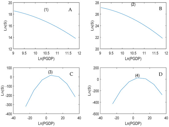
Figure 3.
EKC curve of industrial sulfur dioxide emissions. (A,C) indirect effect EKC, (B,D) total effect EKC, (A,B) is a short-term curve, Figure (C,D) is a long-term curve.
According to Figure 3, the following conclusions can be drawn. First, the direct effect of economic development was not significant, indicating that small-scale local economic development has a limited impact on the industrial sulfur dioxide emission intensity in the region, and larger-scale high-quality economic development is needed to achieve regional environmental improvement. Secondly, the long-term indirect and total effect curves (Figure 3C,D) were inverted “U” types, indicating that with the increase in GDP per capita in the adjacent areas or the whole, the industrial sulfur dioxide emission intensity in the region increases first. After reaching the inflexion point, the industrial sulfur dioxide emission intensity decreases. From the short-term indirect and total effect curves (Figure 3A,B), it can be seen that because the Beijing–Tianjin–Hebei region is one of the more economically developed regions in China and is driven by a high-quality development strategy, the current level of regional economic development has crossed the inflexion point. The growth of per capita GDP will be conducive to curbing industrial sulfur dioxide emission intensity. In addition, the shape of the total effect curve was very similar to the indirect effect curve. In the total effect, the indirect effect plays a more important role. The industrial dynamics of adjacent areas will greatly impact the region’s industrial sulfur dioxide emission intensity. Therefore, to achieve regional, coordinated, high-quality development, it is necessary to rely on the region and achieve a wider range of regional industrial joint interactions and ecological coordinated prevention and control.
4.1.3. The Influence of Control Variables on Industrial Sulfur Dioxide
According to the estimation results (Table 3), among the six control variables, the effects of foreign direct investment, the proportion of scientific research expenditure, and the comprehensive utilization rate of industrial solid are not significant, and at least one of the other variables is significant. Among them, the direct effect of per capita GDP is − 1.244, which is significant at the 1% level. A 1% per capita GDP growth in the region will lead to a 1.244% reduction in the intensity of local industrial sulfur dioxide emissions. The indirect effect is not significant. The total effect is negative and significant, indicating that the increase in per capita GDP is conducive to reducing industrial sulfur dioxide emission intensity. The direct and indirect effects of population size are significant and opposite in sign, indicating that the increase in local population size is conducive to reducing the industrial sulfur dioxide emission intensity in the region, but will increase the industrial sulfur dioxide emission intensity in the adjacent areas. The direct effect and indirect effect are offset, resulting in the total effect of population size on industrial sulfur dioxide emission intensity is not significant. The three effects of the proportion of the secondary industry are positive and significant at the 1% level, indicating that the industrial structure has a significant impact on the intensity of industrial sulfur dioxide emissions. Therefore, adjusting the industrial structure, reasonably reducing the proportion of the secondary industry and vigorously developing the tertiary industry are important measures to solve environmental problems and achieve high-quality development.
4.2. Effect of Industrial Transfer on Industrial Wastewater Discharge Intensity
4.2.1. Influence of Industrial Transfer on Industrial Wastewater
According to the spatial panel data model screening procedure, the spatial Dubin individual fixed effect model was determined as the best model, and the finite distance spatial weight matrix was selected for quantitative analysis. The model estimation results are shown in Table 9.
Table 9.
Estimation results of direct, indirect and total effects of industrial wastewater.
According to the model measurement results (Table 5), the direct effect of the industrial transfer was −0.467, which was significant at the 1% level, indicating that every 1% increase in industrial transfer in the region will lead to a 0.467% reduction in industrial wastewater emission intensity in the region. Undertaking industrial transfer reduces the discharge of industrial wastewater per unit of GDP, indicating that during the current period, the Beijing–Tianjin–Hebei region has adopted stricter environmental regulation policies, and the industrial wastewater discharge intensity of industry is lower than the local average discharge intensity, resulting in a decrease in industrial wastewater discharge intensity. The indirect effect of the industrial transfer was significant at 10%, indicating that industrial transfer has a certain spatial spillover effect on the inhibition of industrial wastewater emission intensity. The total effect value of the industrial transfer was −0.856, which was significant at the 1% level. Overall, the industrial transfer in the Beijing–Tianjin–Hebei region is conducive to reducing the intensity of industrial wastewater discharge. Under a moderate environmental regulation policy, promoting the normal flow of industry can alleviate the problem of industrial wastewater pollution to a certain extent. In the total effect, the direct effect occupied the main position. When solving the problem of industrial wastewater pollution, we should pay attention to the industrial undertakings in the region, and introduce scientific, industrial undertaking policies. Finally, we replaced the original matrix with a 0–1 distance matrix and a spatial matrix based on latitude and longitude, and the empirical results were still robust.
4.2.2. EKC Relationship between Economic Development and Industrial Wastewater
According to the direct, indirect and total effects of per capita GDP [Ln(PGDP), Ln2(PGDP)] (Table 10), the EKC curve of industrial wastewater discharge intensity could be analyzed and decomposed into direct, indirect, and total effect EKC curves (Figure 4). The direct effect curve of industrial wastewater (Figure 4A,D) was a positive “U” type and is currently at the bottom of the U-shaped curve. The increase in per capita GDP may lead to increased industrial wastewater discharge intensity in the region. The indirect effect curve (Figure 4B,E) was an inverted “U” type, and the current curve crosses the inflexion point and is beginning to decline gradually. With the increase in per capita GDP in the adjacent areas, the intensity of industrial wastewater discharge has shown a downward trend. Compared with the direct effect (10% level is significant), the indirect effect (1% level is significant) was more robust. The total effect EKC curve (Figure 4C,F) was also an inverted “U” type. With the development of per capita GDP, the intensity of industrial wastewater discharge is showing a downward trend (Figure 4C). The shapes of the total effect and indirect effect EKC curves were similar, indicating that the indirect effect plays a greater role.
Table 10.
Estimated results of direct, indirect and total effects of industrial wastewater (square).
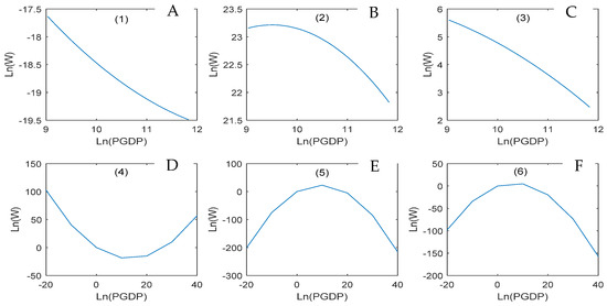
Figure 4.
EKC curve of industrial wastewater discharge. (A,D) direct effect EKC, (B,E) indirect effect EKC, (C,F) total effect EKC, (A–C) are short-term curves, (D–F) are long-term curves (The short-term curve refers to the EKC curve during the study period, and the long-term curve refers to the EKC curve appropriately expanded during the study period.).
4.2.3. Influence of Control Variables on Industrial Wastewater
According to the estimation results (Table 5), among the six control variables, except for the proportion of foreign direct investment and scientific research expenditure, of the three effects of the remaining variables at least one was significant. The direct effect of per capita GDP was –1.791, which was significant at the 1% level, indicating that 1% per capita GDP growth in the region will lead to a 1.791% reduction in local industrial wastewater emission intensity. The indirect effect was 0.729, meaning that neighboring regions’ economic growth may lead to increased industrial wastewater discharge intensity in the region through various channels. The total effect was negative and significant, indicating that the increase in per capita GDP is conducive to the reduction in industrial wastewater discharge intensity, and the direct effect is dominant in the total effect. The three effects of population size significantly impacted the intensity of industrial wastewater discharge. The direct and total effects had the same symbols and had an inhibitory effect on the intensity of industrial wastewater discharge. The neighboring areas’ population size will negatively impact the region’s intensity of industrial wastewater discharge. The direct effect of the proportion of the secondary industry was insignificant, and the indirect effect and the total effect were significant at the 1% level, indicating that the industrial structure significantly impacts the intensity of industrial wastewater discharge. The high proportion of the secondary industry is not conducive to reducing industrial wastewater discharge intensity. Therefore, optimizing the industrial structure, reasonably reducing the proportion of the secondary industry, and vigorously developing the tertiary industry are effective ways to solve environmental problems. The direct effect of the industrial solid comprehensive utilization rate was significantly positive. In contrast, the indirect effect was negative and insignificant, and the total effect was positive and negligible, indicating that the improvement of the industrial solid comprehensive utilization rate has no significant impact on industrial wastewater discharge.
4.3. Effect of Industrial Transfer on Emission Intensity of Industrial Smoke (Dust)
4.3.1. Influence of Industrial Transfer on Industrial Smoke (Powder) Dust
According to the screening procedure of the spatial panel data model, the spatial Dubin individual fixed effect model was determined as the best model, and the finite distance spatial weight matrix was selected to carry out the spatial econometric analysis. The measurement results are shown in Table 11.
Table 11.
Estimation results of direct, indirect and total effects of industrial smoke (powder) dust.
It can be seen from Table 7 that the direct, indirect, and total effects of industrial transfer were all negative, and the direct effect was not significant. In contrast, the indirect and total effects were significant at the 1% level. Overall, the industrial transfer has a significant pollution halo effect, which has an inhibitory effect on industrial smoke (powder) dust emission intensity. The direct effect of per capita GDP was negative, and the indirect effect was positive. Both were significant at the 1% level, indicating that per capita GDP growth is conducive to reducing the intensity of industrial smoke (powder) dust emissions in the region, and may have a stimulating effect on industrial smoke (powder) dust emissions in neighboring areas. However, from the perspective of the total effect, the direct and indirect effects of economic growth were opposite and offset each other, making the total effect insignificant. The effect of population size on industrial smoke (dust) emission intensity was similar to that of per capita GDP. The direct effect was negative, and the indirect effect was positive. The two offset each other, making the total effect insignificant. The direct effect of the proportion of the secondary industry was positive and significant at the 10% level. The indirect effect and total effect were not significant. In addition, foreign direct investment, the proportion of investment in science and technology and industrial solids, and the comprehensive utilization efficiency have no significant impact on industrial smoke (powder) dust emission intensity.
4.3.2. EKC Relationship between Economic Development and Industrial Smoke (Powder) Dust
According to the results shown in Table 12, the total effect of Ln(PGDP) and the indirect and total effects of Ln2(PGDP) were significant, and the indirect and total effect EKC curves of industrial smoke (powder) dust emission intensity could be drawn, as shown in Figure 5. First, the indirect effect EKC curve of industrial smoke (powder) dust emission intensity was an inverted “U” type, with the economic growth of industrial smoke (powder) dust emissions increasing first and then decreasing (Figure 5C). From the current point of view (Figure 5A), the Beijing–Tianjin–Hebei economic development has exceeded the inflexion point, so with the increase of regional per capita GDP, industrial smoke (powder) dust emission intensity will show a downward trend. In addition, the EKC curve of the long-term total effect of industrial smoke (powder) dust was also an inverted “U” shape (Figure 5D), and its inflexion point was 9.258. Only 3.59% of the sample points were located on the left side of the inflexion point; the remaining samples had exceeded the inflexion point (Figure 5B, Table 12).
Table 12.
Estimated results of direct, indirect and total effects of industrial smoke (dust) (square).
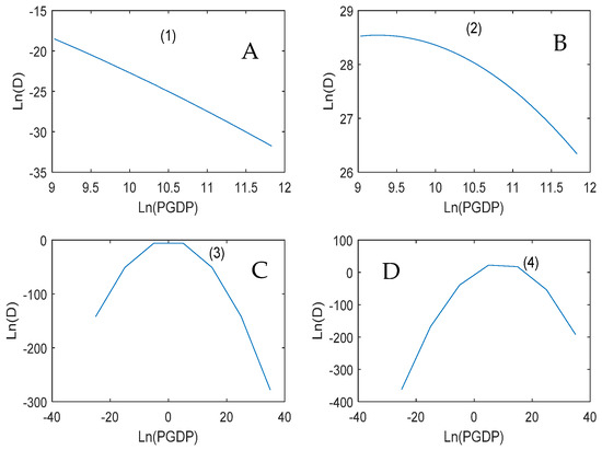
Figure 5.
EKC curve of industrial smoke (dust) emission. Note: (A,C) indirect effect EKC, (B,D) total effect EKC, (A,B) is the short-term EKC curve, (C,D) is the long-term EKC curve.
Finally, we replaced the original model’s finite distance spatial weight matrix with the 0–1 spatial weight matrix and the spatial weight matrix based on latitude and longitude, and carried out a robustness test analysis. The core explanatory variables (industrial transfer) obtained by the three spatial weight matrices had the same impact on industrial smoke (powder) dust. The robustness test results of Table 12 (including square terms) also proved that the model estimation satisfies robustness.
5. Conclusions
This paper explored the impacts of industrial transfer on the environment in the Beijing–Tianjin–Hebei region, and constructed the direct EKC, indirect EKC, and total EKC. The results showed that industrial transfer has an inhibitory effect on the emission intensity of three types of industrial pollutants. The direct and indirect effects of industrial transfer have a significant inhibitory effect on industrial wastewater, whereas only the indirect effect of industrial transfer will reduce the emission intensity of industrial sulfur dioxide and soot. Industrial sulfur dioxide, wastewater, and soot all have an inverted U-shaped indirect effect and total effect EKC curves. In addition, industrial wastewater also has a positive U-shaped direct effect EKC curve. In terms of control variables, the impact of economic growth, population size, industrial structure, foreign direct investment, and technological level on the emission intensity of different pollutants was also found to be slightly different, and the direct and indirect effects on the emission intensity of the same pollutant may also be different, but the proportion of secondary production has a positive impact on each pollutant. Therefore, optimizing the industrial structure is a common way to solve all kinds of pollution. Environmental change results from the combined effect of multiple factors and the direction and effect of different factors on the environmental impact are different. Therefore, it is necessary to introduce targeted environmental policies jointly managed and developed together between regions, maximize the benefits of industrial transfer, relieve Beijing’s non-capital functions, and realize the coordinated development of the environment and economy in the Beijing–Tianjin–Hebei region.
6. Suggestions
Industrial transfer has an influential effect on the discharge of different pollutants, and there are differences in the indirect effect and direct effect of industrial transfer. In the control variable, the proportion of the secondary industry had a positive impact on each pollutant, and there was a U-shaped relationship between various pollutants and economic development. Based on the above research findings, this paper proposes the following recommendations.
First, we must promote orderly Beijing–Tianjin–Hebei region industrial transfer. The coordinated development of Beijing–Tianjin–Hebei will ease the non-capital function of Beijing as the starting point, adjust and optimize the urban layout and spatial structure, and expand the environmental capacity. According to the five development concepts, Beijing–Tianjin–Hebei will develop into a world-class urban agglomeration with the capital as the core. It will be a leading area for regional coordinated development and reform, a new engine for national innovation-driven economic growth, and a demonstration area for ecological restoration and environmental improvement. According to functional orientation, all pollution-intensive industries in Beijing, Zhangcheng, and adjacent areas to Beijing and Xiong’an will be eliminated or relocated, and all high-pollution enterprises in Tianjin will be eliminated or relocated. Other regions in Hebei will upgrade, eliminate, transfer, and retain a batch of high-pollution enterprises according to ecological and economic conditions. The environmental capacity will be far greater than the emissions of pollution-intensive enterprises.
Second, joint prevention and treatment should target environmental governance. The coordinated development of the Beijing–Tianjin–Hebei region, including economic and ecological coordination, currently only considers the region’s environmental prevention and control and cannot fundamentally solve ecological problems. Collaborative economic development, environmental joint prevention and control, and vigorous promotion of the integration of green growth in the Beijing–Tianjin–Hebei region will contribute to the integrated protection and restoration of mountains, rivers, forests, fields, lakes, and grasslands, and the integration of mountain control, water control, gas control, and city control. The Hebei Zhangcheng area should become a green ecological industrial belt. Most of the pollution-intensive industries in Beijing and Tianjin, and the Xiong’an adjacent areas, have already been relocated. The distribution density of pollution-intensive enterprises in Baoding, Shijiazhuang, Xingtai, Handan, Tangshan, and Cangzhou is large, and the excess capacity can be reasonably transferred to other regions or overseas regions. This region can be built into a demonstration area for upgrading and transforming traditional industries and developed into an advanced manufacturing industry belt. Different and targeted control and prevention measures should be taken for air pollution, water pollution, and solid waste pollution. In addition, through the coordination of fiscal, taxation, and financial policies, we must strictly control key polluting enterprises, increase preferential compensation for energy conservation and environmental protection industries, and form a systematic ecological mechanism for the coordinated development of Beijing–Tianjin–Hebei industries.
Third, the industrial structure should be adjusted and the industrial layout optimized. The empirical results showed that appropriately reducing the proportion of secondary industry and vigorously developing tertiary industry is conducive to solving environmental problems in the region and neighboring regions. In the early stage of industrialization, the Beijing–Tianjin–Hebei region, especially Hebei Province, developed a large number of heavy industries. Economic development has also caused many environmental problems; however, the Beijing–Tianjin–Hebei region has entered a post-industrial era, transforming from extensive economic growth to high-quality development, and steadily promoting the construction of ecological civilization has become the main theme of the Beijing–Tianjin–Hebei region, and even the whole country. In central and southern Hebei, the distribution density of pollution-intensive industries remains large, and the climatic conditions are not conducive to atmospheric circulation, making extreme haze pollution a risk. Central and southern Hebei should take measures such as industrial relocation and upgrading of traditional industries to reduce the distribution density of pollution-intensive enterprises, vigorously develop tertiary industry, adjust the industrial structure, and optimize the industrial layout. In addition, in the process of structural adjustment and transformation and upgrading, Beijing–Tianjin–Hebei industry must address the restrictions of administrative divisions, weaken the isomorphism of the three regional industries, and unify the planning and coordination of the management of the region, including the industrial structure, industrial layout, industrial docking, industrial integration, industrial transfer, and industrial transformation and upgrading.
Fourth, we must improve the level of circular economy development. The research results showed that a circular economy is an effective way to solve environmental problems. The circular economy is an important breakthrough to realizing the coordinated development of the economy and environment. It plays an irreplaceable role in reducing pollutant emissions and energy consumption, developing strategic emerging industries, and protecting the ecological environment. The development of a circular economy can comprehensively improve resource utilization efficiency by building a multi-level resource recycling system. In the field of industrial production, the five major tasks of green design of key products, clean production of key industries, circular development of parks, comprehensive utilization of resources, and coordinated disposal of urban waste have been gradually completed. The major tasks include improving the level of processing and utilization of renewable resources, standardizing the development of the second-hand commodity market, and promoting the high-quality development of the remanufacturing industry. In addition, the development of a circular economy requires strengthening the monitoring and evaluation of resource utilization efficiency, and improving the statistical data supporting the development of the circular economy. Specifically, in central and southern Hebei, the original industrial park will be transformed into a circular economy eco-industrial park, with “reduction, reuse, recycling” as the principle, to change the past “mass production, mass consumption, abandon” traditional model.
Fifth, we must promote green production and lifestyles, and explore the road to high-quality development. The Beijing–Tianjin–Hebei region should vigorously promote green production and lifestyles, establish co-construction and sharing, and promote green consumption, travel, and green living. Green production is a comprehensive measure to implement pollution control in the whole process of industrial production, with the goal of saving energy, reducing consumption, and reducing pollution, using management and technology as the means. A green lifestyle is a resource-saving and environmentally friendly modern civilized lifestyle, and advocates green consumption, green travel, and green living. It is a profound change in ideas, consumption patterns, and social governance. It will force production methods to achieve green transformation. Promoting the green transformation of production and lifestyle represents a profound change in development concepts and practices. First, we must adhere to and implement new development concepts, correctly handle the relationship between economic development and ecological and environmental protection, and resolutely abandon development models that damage or destroy the ecological environment. Second, we must build an ecological economic system with industrial ecologicalization and ecological industrialization as the main body, and take the road of green, low-carbon, and circular development. We must establish a new outlook on survival and happiness, and we must advocate green consumption in order to achieve sustainable utilization of resources. Specifically, the Beijing–Tianjin–Hebei region has the basic conditions for the transformation to high-quality development. The consumer demand in the region is growing, the service industry is developing rapidly, and the scale of middle-income groups is increasing. Supply side structural reform will drive the Beijing–Tianjin–Hebei region to achieve high-quality development.
Author Contributions
S.X.: Conceptualization, methodology, validation, formal analysis, investigation, resources, writing—original draft, writing—review and editing. L.F.; conceptualization, software, validation, writing—review and editing, visualization, supervision, funding acquisition. S.S.; conceptualization, validation, writing—review and editing, data curation, project administration. All authors have read and agreed to the published version of the manuscript.
Funding
This research was funded by the Key Topics of Statistical Research of Guizhou Provincial Bureau of Statistics in 2022 (No: Z202201), the Guizhou Key Laboratory of Big Data Statistical Analysis (No: BDSA20200109), the Talent Introduction Fund of Guizhou University of Finance and Economics (No: 2018YJ68), and the Humanities and Social Science Research Project of Hebei Education Department (No: BJ2017089).
Institutional Review Board Statement
Not applicable.
Informed Consent Statement
Not applicable.
Data Availability Statement
Data of all indicators come from China Industrial Statistical Yearbook, China Urban Statistical Yearbook, China Environmental Statistical Yearbook, China Statistical Yearbook, provincial statistical yearbook, and EPS data platform.
Acknowledgments
The views and opinions expressed in this article are those of the individual authors.
Conflicts of Interest
The authors declare no conflict of interest.
References
- Sarkodie, S.A.; Strezov, V. A review on environmental Kuznets curve hypothesis using bibliometric and meta-analysis. Sci. Total Environ. 2019, 649, 128–145. [Google Scholar] [CrossRef] [PubMed]
- Antonakakis, N.; Chatziantoniou, I.; Filis, G. Energy consumption, CO2 emissions, and economic growth: An ethical dilemma. Renew. Sustain. Energy Rev. 2017, 68, 808–824. [Google Scholar] [CrossRef]
- Robert, J.R. Are ASEAN countries havens for Japanese pollution-intensive industry? World Econ. 2008, 31, 236–254. [Google Scholar]
- Sun, C.; Zheng, S.; Wang, J.; Kahn, M.E. Does clean air increase the demand for the consumer city? Evidence from Beijing. J. Reg. Sci. 2019, 59, 409–434. [Google Scholar] [CrossRef]
- Akbostanci, E.; Tunc, G.I.; Türüt-Aşik, S. Pollution haven hypothesis and the role of dirty industries in Turkey’s exports. Environ. Dev. Econ. 2007, 12, 297–322. [Google Scholar] [CrossRef]
- Li, Y. Path-breaking industrial development reduces carbon emissions: Evidence from Chinese Provinces 1999–2011. Energy Policy 2022, 167, 113046. [Google Scholar] [CrossRef]
- Silva, E.C.D.; Zhu, X. Emissions trading of global and local pollutants, pollution havens and free riding. J. Environ. Econ. Manag. 2009, 58, 169–182. [Google Scholar] [CrossRef]
- Wang, H.; Dong, C.; Liu, Y. Beijing direct investment to its neighbors: A pollution haven or pollution halo effect? J. Clean. Prod. 2019, 239, 118062. [Google Scholar] [CrossRef]
- Albornoz, F.; Cole, M.A.; Elliott, R.J.R.; Ercolani, M.G. In search of environmental spillovers. World Econ. 2009, 32, 136–163. [Google Scholar] [CrossRef]
- Dardati, E.; Saygili, M. Multinationals and environmental regulation: Are foreign firms harmful? Environ. Dev. Econ. 2012, 17, 163–186. [Google Scholar] [CrossRef]
- Mert, M.; Caglar, A.E. Testing pollution haven and pollution halo hypotheses for Turkey: A new perspective. Environ. Sci. Pollut. Res. 2020, 27, 32933–32943. [Google Scholar] [CrossRef] [PubMed]
- Kisswani, K.M.; Zaitouni, M. Does FDI affect environmental degradation? Examining pollution haven and pollution halo hypotheses using ARDL modelling. J. Asia Pac. Econ. 2021, 7, 1–27. [Google Scholar] [CrossRef]
- Kirchherr, J.; Matthews, N. Technology transfer in the hydropower industry: An analysis of Chinese dam developers’ undertakings in Europe and Latin America. Energy Policy 2018, 113, 546–558. [Google Scholar] [CrossRef]
- Grossman, G.M.; Krueger, A.B. Economic growth and the environment. Q. J. Econ. 1995, 110, 353–377. [Google Scholar] [CrossRef]
- Bibi, F.; Jamil, M. Testing environment Kuznets curve (EKC) hypothesis in different regions. Environ. Sci. Pollut. Res. 2021, 28, 13581–13594. [Google Scholar] [CrossRef] [PubMed]
- Onafowora, O.A.; Owoye, O. Bounds testing approach to analysis of the environment Kuznets curve hypothesis. Energy Econ. 2014, 44, 47–62. [Google Scholar] [CrossRef]
- Lin, B.; Zhu, J. Changes in urban air quality during urbanization in China. J. Clean. Prod. 2018, 188, 312–321. [Google Scholar] [CrossRef]
- Dijkgraaf, E.; Vollebergh, H.R.J. A test for parameter homogeneity in CO2Panel EKC estimations. Environ. Resour. Econ. 2005, 32, 229–239. [Google Scholar] [CrossRef]
- Ersin, Ö.; Bildirici, M. Asymmetry in the environmental pollution, economic development and petrol price relationship: MRS-VAR and nonlinear causality analyses. Rom. J. Econ. Forecast 2019, 22, 25–50. [Google Scholar]
- Hassan, S.A.; Nosheen, M.; Rafaz, N. Revealing the environmental pollution in nexus of aviation transportation in SAARC region. Environ. Sci. Pollut. Res. 2019, 26, 25092–25106. [Google Scholar] [CrossRef]
- Barquín, R. A sceptical vision of the environmental Kuznets curve: The case of sulfur dioxide. Int. J. Sustain. Dev. World Ecol. 2006, 13, 513–524. [Google Scholar] [CrossRef]
- Baek, J.; Kim, H.S. Is economic growth good or bad for the environment? Empirical evidence from Korea. Energy Econ. 2013, 36, 744–749. [Google Scholar] [CrossRef]
- Lee, S.; Oh, D.W. Economic growth and the environment in China: Empirical evidence using prefecture level data. China Econ. Rev. 2015, 36, 73–85. [Google Scholar] [CrossRef]
- Renzhi, N.; Baek, Y.J. Can financial inclusion be an effective mitigation measure? Evidence from panel data analysis of the environmental Kuznets curve. Financ. Res. Lett. 2020, 37, 101725. [Google Scholar] [CrossRef]
- Bildirici, M.; Ersin, Ö. Markov-switching vector autoregressive neural networks and sensitivity analysis of environment, economic growth and petrol prices. Environ. Sci. Pollut. Res. 2018, 25, 31630–31655. [Google Scholar] [CrossRef]
- Liu, T.; Pan, S.; Hou, H.; Xu, H. Analyzing the environmental and economic impact of industrial transfer based on an improved CGE model: Taking the Beijing–Tianjin–Hebei region as an example. Environ. Impact Assess. Rev. 2020, 83, 106386. [Google Scholar] [CrossRef]
- LeSage, J.P.; Pace, R.K. Spatial econometric models. In Handbook of Applied Spatial Analysis; Springer: Berlin/Heidelberg, Germany, 2010; pp. 355–376. [Google Scholar]
- Chen, H.; Dong, K.; Wang, F.; Ayamba, E.C. The spatial effect of tourism economic development on regional ecological efficiency. Environ. Sci. Pollut. Res. 2020, 27, 38241–38258. [Google Scholar]
- Jena, P.R.; Bildirici, M.; Ritanjali, M. Estimating Long-Run Relationship between Renewable Energy Use and CO2 Emissions: A Radial Basis Function Neural Network (RBFNN) Approach. Sustainability 2022, 14, 5260. [Google Scholar] [CrossRef]
- Elhorst, J.P. Spatial Panel Data Analysis. Encycl. GIS 2017, 2, 2050–2058. [Google Scholar]
- Wang, Y.; Wang, X.; Chen, W.; Qiu, L.; Wang, B.; Niu, W. Exploring the path of inter-provincial industrial transfer and carbon transfer in China via combination of multi-regional input–output and geographically weighted regression model. Ecol. Indic. 2021, 125, 107547. [Google Scholar] [CrossRef]
- Feng, L.; Shang, S.; Feng, X.; Kong, Y.; Bai, J. Evolution and Trend Analysis of Research Hotspots in the Field of Pollution-Intensive Industry Transfer—Based on Literature Quantitative Empirical Study of China as World Factory. Front. Environ. Sci. 2022, 8, 428. [Google Scholar] [CrossRef]
- Stossel, Z.; Kissinger, M.; Meir, A. Assessing the state of environmental quality in cities–a multi-component urban performance (EMCUP) index. Environ. Pollut. 2015, 206, 679–687. [Google Scholar] [CrossRef] [PubMed]
- Zhou, A.; Li, J. Impact of income inequality and environmental regulation on environmental quality: Evidence from China. J. Clean. Prod. 2020, 274, 123008. [Google Scholar] [CrossRef]
- Zhou, W.; Yang, W.; Wan, W.; Zhang, J.; Yang, H.-S.; Yang, H.; Xiao, H.; Deng, S.-H.; Shen, F.; Wang, Y.-J. The influences of industrial gross domestic product, urbanization rate, environmental investment, and coal consumption on industrial air pollutant emission in China. Environ. Ecol. Stat. 2018, 25, 429–442. [Google Scholar] [CrossRef]
- Ahmad, F.; Draz, M.U.; Chandio, A.A.; Ahmad, M.; Su, L.; Shahzad, F.; Jia, M. Natural resources and environmental quality: Exploring the regional variations among Chinese provinces with a novel approach. Resour. Policy 2022, 77, 102745. [Google Scholar] [CrossRef]
- He, L.; Wu, M.; Wang, D.; Zhong, Z. A study of the influence of regional environmental expenditure on air quality in China: The effectiveness of environmental policy. Environ. Sci. Pollut. Res. 2018, 25, 7454–7468. [Google Scholar] [CrossRef]
- Elhorst, J.P. Serial and spatial error dependence in space-time models. In Spatial Econometrics and Spatial Statistics; Palgrave Macmillan: London, UK, 2004; pp. 176–193. [Google Scholar]


Publisher’s Note: MDPI stays neutral with regard to jurisdictional claims in published maps and institutional affiliations. |
© 2022 by the authors. Licensee MDPI, Basel, Switzerland. This article is an open access article distributed under the terms and conditions of the Creative Commons Attribution (CC BY) license (https://creativecommons.org/licenses/by/4.0/).