Controller Development and Experimental Validation for a Vertical Axis Wind Turbine

Abstract

This paper reports experimental results, in a wind tunnel, of controllers for a vertical axis wind turbine (VAWT). Models and controllers from previous works were validated and improved through the acquisition of new data sets. The control methods used are PID, LQR and CRONE (a type of fractional order control, i.e., a controller using fractional derivatives). The simulation results led to the choice of the CRONE controller for implementation. Hardware and software were developed to perform tests in a wind tunnel, that proved the correct behavior of the controller whilst validation results exceeded those from simulation. These results are expected to contribute for the viability of VAWTs in urban environments since they can aid in the increasing demand of energy services in urban areas without increasing the carbon emission levels of the area.

1. Introduction

Due to concerns related to the environment, the interest in renewable energy sources has been steadily increasing in order to successfully transition the energy production to become more environmentally friendly, with much lower carbon emissions. Wind energy is one of these sources, being one of the highest average growth rate sectors, second only to solar power, among countries in the Organization for Economic Co-operation and Development (OECD) [1].

While the concept of a wind turbine has existed since the 19th century, its technology is under constant development as manufacturing and control methods are improved. At the same time, new problems in its implementation are being discovered, as unintended or unforeseen consequences are still being uncovered. A wind turbine’s advantages include a renewable, sustainable and never ending resource, and the ability to provide power to remote locations where other sources of energy might be impractical or too expensive to reach or exploit. On the other hand, the wind itself fluctuates in intensity; thus, the power production is not constant, leading to the necessity of energy storage in case of energy shortages. Furthermore, due to its constant rotation, the blades might need constant maintenance and eventual replacement due to erosion. Another disadvantage of the commonly used wind turbines nowadays is their size, which in turn means its components are very large, requiring specialized transportation and complex logistics for installation and component replacement.

These wind turbines possess a horizontal rotational axis, thus they will be referred to as horizontal axis wind turbines (HAWT) from this point onward. Due to their size, wind farm installation near an urban area is impractical, thus a vertical axis wind turbine (VAWT) may be the solution for electricity production in such sites, closer to where energy demand is larger. These wind turbines, VAWTs, possess some advantages over the traditional HAWTs [2] such as:

• Their natural independence of the wind flow direction translates into a lower number of components;
• They possess a smaller size, thus requiring lower logistical effort in their installation and easing the required maintenance.

Yet VAWTs are not void of disadvantages such as producing less power when compared to the traditionally used HAWT, and they inherit some of HAWTs’ disadvantages such as the blades’ erosion problem. Nevertheless, interest in and development of VAWT-related technology has been increasing due to the previously mentioned advantages over HAWTs.

1.1. State of the Art

A few studies were conducted to analyze the performance of VAWT installations in an urban context. In [3], a more traditional approach was performed, resorting to data acquisition through anemometers and a wind tunnel, while in [4] the data was acquired through a computational fluid dynamics (CFD) calculation of flow velocity and skew angle on the rooftop of several buildings. In [5], several configurations of a Darrieus-type VAWT are described, along with some of their characteristics, drawbacks and advantages.

VAWTs can be mainly categorized as two types: Darrieus or Savonius. While a Darrieus-type VAWT uses an angle of attack on its blade to spin, a Savonius type is simpler, as it spins using drag, also having a much lower self starting wind speed requirement. One advantage of a Savonius-type turbine over a Darrieus-type turbine is its low self-start wind speed requirement. Related to this drawback, a new methodology for development of new blade profiles for self-start Darrieus wind turbines is presented in [6], for symmetrical airfoils, and in [7] for asymmetrical airfoils. In [8], a hybrid Darrieus–Savonius turbine is proposed, although the expected performance was not achieved.

A new approach to a type of model called Double Multiple Streamtube (DMS) is presented in [9], aiming to present an easy tool for the study of complex-shaped VAWT blades, able to be integrated in computational modeling tools. Other methods for improving the characteristics of existing turbines without modifications on the turbine itself were studied. A study performed in [10] concluded that an increase in the rotational speed of the VAWT occurs with the installation of an omni-directional-guide-vane, in an urban context, improving the power output and diminishing the visual impact of wind turbines. An alternative to installing omni-directional-guide-vanes is a ducted turbine. In [11], a study was performed, predicting very high specific power output and having clear advantages, namely the visual impact and safety. Despite these advantages, it has a clear drawback, which is its directional sensitivity.

Regarding the implementation of control strategies, a control technique for a sensorless application to maximize the power output up to the rated wind speed of a VAWT using a permanent magnet synchronous generator (PMSG) is proposed in [12], whose results are presented on an equivalent circuit model in the Simulink environment. A model is proposed in [13], considering a variable speed wind turbine, two mass rotor, a PMSG and different power converters, providing a new control strategy based on fractional-order controllers. The model is considered more realistic and accurate, and simulation results show that the proposed control strategy improves disturbance attenuation and system robustness.

In [14], different power converters are studied, modeled and compared in simulation, considering more accurate dynamics regarding the turbine and its connection to the electric network. In [15], variable-speed wind turbines equipped with PMSG are modeled and studied, simulating a malfunction and the controller’s response resorting to traditional and fractional PI, comparing their performance.

New blades for a VAWT are developed in [16] with the objective of improving the self-start characteristics without the aid of any additional component. These blades exhibit good performance for wind speeds below 25 m/s, without significant drawbacks such as instability and vibrations. From these blades, a VAWT prototype was developed, which was studied further in [17] with the identification of mathematical models and control development resorting to PID and LQR methods. Further controllers for the same prototype are given in [18], resorting to fractional control, more precisely using the CRONE control method. From the latter work came the need to validate the previous results through testing in a controlled environment such as a wind tunnel.

These works, whilst numerous, prove that technology regarding VAWT applications is still in development and far from being economically viable for their installation in urban areas, which are increasing the energy demands as time passes.

1.2. Objectives

Thus, to successfully achieve the objective of control validation, the following stages were accomplished in order:

• Validate the models previously obtained in [17] or create new models resorting to recently acquired data;
• Validate controllers previously obtained or create new controllers, depending on the results of the previous stage;
• Compare the performance of controllers in simulation;
• Choose the best option for implementation, developing the required software and hardware;
• Test the controller in a controlled environment for different wind speeds.

In summary, this paper follows the same line of thought as in [19] with a comparison between simulation and experimental results in order to extract conclusions regarding the system’s performance.

This paper presents the Darrieus wind turbine addressed in Section 2. Section 3 presents and discusses the results of the above stages of the work. Section 4 provides possible actions to further improve the results obtained by this work.

2. Materials and Methods

The following overview of the generator sums up the extensive exposition in [17]. Most VAWTs consist of:

• rotor;
• drivetrain;
• generator;
• tower;
• control system;

with the latter being the main focus of this work. The control system is comprised of sensors, actuators, a central processing unit and controllers, and the flowchart, presented in Figure 1, represents a simplified version of the turbine’s wind energy conversion system.

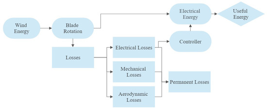
Figure 1. Flowchart representation of the prototype’s energy conversion system.

While the prototype, together with its components, was developed in previous works as already mentioned, it nevertheless required some maintenance and some components needed replacement. The component acting as the central processing unit, an Arduino UNO, was replaced by an Arduino MEGA 2560 (Arduino, Monza, Italy), seen in Figure 2a, due to its higher processing capabilities compared to the previously used Arduino; the actuators were also replaced by better servos, with higher torque and precision, model Servo TowerPro MG995 (TowerPro, Singapore) ${270}^{\circ }$, seen in Figure 2b at the base of the aluminum case.

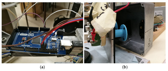
Figure 2. CPU and Actuators: (a) Arduino MEGA; (b) Servo.

The sensors that will read the input data for the controller are an anemometer and an infrared sensor, responsible for transmitting the wind velocity and turbine’s angular velocity, respectively, as seen in Figure 3.

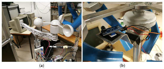
Figure 3. Sensors: (a) anemometer; (b) infrared sensor.

These sensors will send their respective digital signals to the Arduino, which in turn will transform the digital signal into the respective wind speed and turbine angular speed values. The anemometer’s digital signal conversion occurs with every switch closure, with the rate of 1 switchclosure/second $=2.4$ km/h [20], while the conversion rate of the infrared sensor’s digital signal takes the form of the following equation:

$$\omega =\frac{2\pi }{5\Delta t}\mathrm{rad}/\mathrm{s},$$

(1)

since the turbine possesses 5 blades, thus the same number of arms, and $\Delta t$ represents the time between consecutive interruptions. The last components that remain to be mentioned are the rheostats. These are simple rotational rheostats, with a rotation angle of $[0$, $270]$${}^{\circ }$ and resistance values of $[0$, $200]$$\Omega$. With these components, the acquisition of new data sets was made possible, with the aim of using the data to validate or create new models resorting to system identification methods. In order to save the data from the sensors, as are read by the Arduino, a laptop was connected to the Arduino through an USB port. Running in the laptop, through Simulink, was a file, as seen in Figure 4, which took the data sets and recorded it in Matlab R2020a’s workplace.

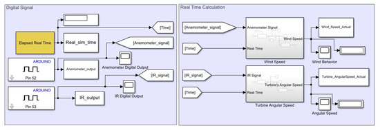
Figure 4. Simulink file used for data acquisition purposes.

The two larger subsystems are responsible for the real time conversion of the digital signal read by the Arduino to the values of wind speed intensity and turbine angular speed, corresponding to the top and bottom subsystems, respectively.

In order to minimize possible errors, a procedure was adopted for the acquisition of data sets. This procedure can be seen in the Appendix A. Table 1 and Table 2 present lists of the values of resistance and wind speed imposed when collecting the experimental data, together with the corresponding measured values. Errors are small, with small average value (−0.26 $\Omega$ and $1.5\times {10}^{-3}$ m/s) and small standard deviation ($0.92$$\Omega$ and $0.013$ m/s); nominal values can consequently be used.

Table 1. Full list of data sets.

		Theoretical Resistance Values
		R $=0\Omega$	R $=10\Omega$	R $=20\Omega$	R $=30\Omega$	R $=40\Omega$	R $=50\Omega$	R $=100\Omega$	R $=150\Omega$	R $=200\Omega$
Initial Value	R${}_1$	−	$9.72$	$19.99$	$30.40$	$40.03$	$50.24$	$99.69$	$150.36$	$199.65$
	R${}_2$	−	$9.95$	$20.09$	$30.07$	$39.92$	$49.89$	$99.44$	$150.40$	$196.49$
	R${}_3$	−	$9.70$	$20.09$	$30.06$	$39.85$	$50.52$	$99.74$	$150.27$	$200.38$
Final Value	R${}_1$	$0.27$	$9.68$	$20.05$	$28.88$	$40.84$	$49.76$	$99.96$	$150.44$	−
	R${}_2$	$0.23$	$7.51$	$20.03$	$28.60$	$39.37$	$47.69$	$100.13$	$149.28$	−
	R${}_3$	$0.25$	$9.31$	$19.37$	$29.23$	$37.89$	$52.36$	$99.39$	$150.28$	−

Table 2. Wind velocity variation data.

	Wind Velocity Value [m/s]
Theoretical	$6.6$	7	8	9	10	11	12	11	10	9	8	7	$6.6$
Real	$6.60$	$6.99$	$7.98$	$9.02$	$10.01$	$11.01$	$12.00$	$11.01$	$10.01$	$9.02$	$7.98$	$6.99$	$6.60$

An example of a single data set, corresponding to a resistance of 200 $\Omega$, is presented in Figure 5. It can be seen that the sensor’s readings are significantly affected by noise; thus, a filter must be applied before the data can be used. The choice fell on a Butterworth filter with cut-off frequency and order determined from the performance index known as root mean square deviation (RMSD):

$$\mathrm{RMSD}=\sqrt{\frac{{\sum }_{t=1}^T{(y_t-z_t)}^2}{T}},$$

(2)

where $y_t$ is the unfiltered data, $z_t$ is the Butterworth filtered data, with a certain cut-off frequency and order, and T is the number of times the value is observed. As the index is to be applied for different wind velocity values, a normalized root mean square deviation (NRMSD) is calculated in order to be able to compare the data uniformly. The NRMSD is given by:

$$\mathrm{NRMSD}=\frac{\mathrm{RMSD}}{{\overline{y}}_t},$$

(3)

where ${\overline{y}}_t$ is the average value of the unfiltered data.

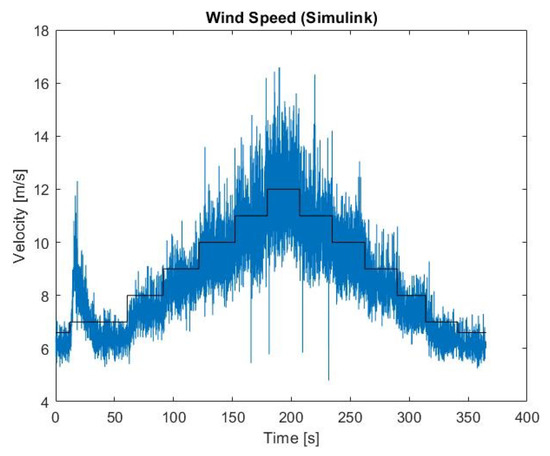
Figure 5. Wind speed data variation read by the anemometer. Blue: wind velocity measured with the anemometer; black: desired wind speed value as found in Table 2.

By calculating the value of NRMSD as a function of the cut-off frequency, from $0.20$ rad/s to $1.00$ rad/s with increments of $0.05$ rad/s, for several different filter’s orders, the following results are obtained, presented by Figure 6, for a wind velocity value of 9 m/s.

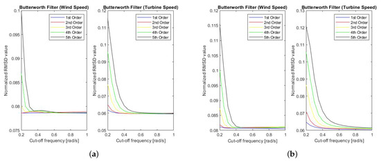
Figure 6. NRMSD values as function of cut-off frequency: (a) for $t=125$ to 150 s; (b) for $t=250$ to 275 s.

It is worth mentioning that these results are from the data set presented in Figure 5 and that the results for other data sets are very similar to the one presented in Figure 6, although the results get worse when applied to the extreme values of the wind velocity presented in Table 2, i.e., $6.6$ m/s and 12 m/s.

Through these results, the desired specifications for the Butterworth filter are:

• Cut-off frequency $=0.40$ rad/s;
• Order $=2$ and 3, since both are used for model identification purposes.

3. Results

This section presents the results from the comparison of previously obtained models with recently identified models resorting to the newly acquired data sets. The comparison of the controllers, the implementation and testing results are also presented.

3.1. Previous Models

From [17], the following 3rd and 2nd order models for the prototype were identified:

$$\Delta \omega \left(s\right)=\frac{0.2214s^2+0.00256s+7.593\times {10}^{-5}}{s^3+0.1564s^2+0.001808s+3.36\times {10}^{-5}}\Delta v\left(s\right)+\frac{0.001159s+1.5\times {10}^{-6}}{s^3+10.43s^2+2.25s+7.5\times {10}^{-4}}\Delta R_c\left(s\right),$$

(4)

$$\Delta \omega \left(s\right)=\frac{7131s+2879.9}{s^2+13200s+1861}\Delta v\left(s\right)+\frac{952s+61.41}{s^2+13200s+1861}\Delta R_c\left(s\right).$$

(5)

These models will be compared with recently identified models in order to verify their performance resorting to the acquired data sets.

3.2. New Models

Following the same structure as the previously presented models, the new models will be a sum of two terms, one with respect to the wind velocity variation $\Delta v\left(s\right)$, which is the disturbance variable, and the other to the imposed resistance variation, $\Delta R_c\left(s\right)$, which will be the control variable, whilst $\Delta \omega \left(s\right)$ is the output variable. Matlab’s system identification toolbox and command systemIdentification were used for this purpose.

3.2.1. $\frac{\Delta \omega \left(s\right)}{\Delta v\left(s\right)}$ Identified Model

Starting with the first term, Table 3 presents the best results from the toolbox. The comparison value will be the fit range of each model, which determines the agreement between the model’s response and the measured output, with 0 indicating a poor fit where the model output is the same as the mean value of the measured output [21].

Table 3. Best fits for $\frac{\Delta \omega \left(s\right)}{\Delta v\left(s\right)}$ transfer functions.

Butterworth Filtered Data Order
$n=\mathbf{3}$				$n=\mathbf{2}$
$R_c$$[\Omega ]$	N° Poles	N° Zeros	Fit Range	$R_c$$[\Omega ]$	N° Poles	N° Zeros	Fit Range
150	3	1	95.1–87.4	50	3	2	94.6–85.3
50	3	1	94.7–87.8	40	3	2	95.4–84.3
30	3	2	96.4–87.2	40	3	1	96.3–85.9
200	2	1	87.8–55.3	0	3	1	95.0–87.9
100	2	1	86.8–59.8	200	2	1	87.7–52.6
50	2	1	86.3–69.4	150	2	1	87.3–54.4
40	2	1	85.5–65.0	50	2	1	86.2–70.1
–	–	–	–	30	2	1	84.2–66.8

From Table 3, and comparing the Bode diagram and step response of each model, it is concluded that models with best results were the following:

• For a 2nd order model: resistance 50 $\Omega$, 2 poles, 1 zero, and filter order 2;

  $$r50\_2\_1\_2\left(s\right)=\frac{0.682s+0.01027}{s^2+0.5484s+0.007979},$$

  (6)
• For a 3rd order model: resistance 40 $\Omega$, 3 poles, 1 zero, and filter order 2;

  $$r40\_3\_1\_2\left(s\right)=\frac{5.707s+0.003067}{s^3+15.87s^2+3.675s+0.002303}.$$

  (7)

3.2.2. $\frac{\Delta \omega \left(s\right)}{\Delta R_c\left(s\right)}$ Identified Model

Whilst the identification of the previous term was performed resorting to the acquired data sets directly, the data sets could not be used directly for this term as a relationship between the resistance’s variation and turbine’s angular speed had to be created. Data manipulation was required before the use of Matlab R2020a’s system identification toolbox could be used.

For the purpose of creating new data sets resorting to the available ones, the following steps were taken:

• From the available data, segments where the wind velocity is stable were identified;
• With the segments identified, their respective turbine angular speed is removed;
• Segments that possess the same wind speed value are joined, creating a continuous line with respect to the desired resistance variation;
• The turbine’s angular speed is normalized in order to remove the wind speed contribution;
• In order to remove the initial signal rise, as it is an undesired dynamic, the minimum resistance value was set as 20 $\Omega$.

The experimental procedure did not include changing the resistance while keeping the wind speed constant because the servos were not available; in fact, identification results were necessary to choose part of the instrumentation of the turbine.

With these steps, new data sets are created where the angular speed varies in function of the resistance’s variation. An example of such data sets can be seen in Figure 7, corresponding to the constant wind velocity of 9 m/s.

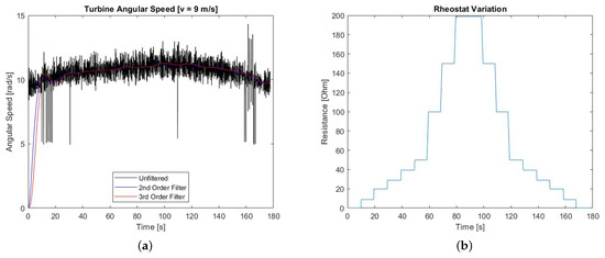
Figure 7. Example of a data set with constant wind velocity: (a) turbine’s angular speed, not normalized; and (b) resistance variation.

One last step was required for the purpose of simulating a real variation speed for the rheostat. In order to remove the instant changes of values, a slope was created between each resistance value change. The slope’s value is given by:

$$R_{speed}=\frac{200}{270}\times (\frac{1}{60}{)}^{-1}\Omega /\mathrm{s},$$

(8)

where $\frac{200}{270}$ refers to the physical limitations of the rheostat itself and $\frac{1}{60}$ is the assumed servo speed. This rotational speed for the servo was taken from the technical data sheet of the component [22], according to the value of operating speed with $4.8$ V and assuming a load imposed by the rheostat. The final data sets are presented by Figure 8.

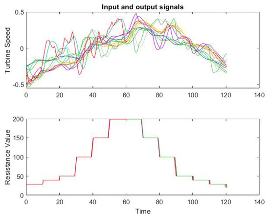
Figure 8. Data sets for the purpose of $\frac{\Delta \omega \left(s\right)}{\Delta R_c\left(s\right)}$ model identification.

From Table 4, and through the comparison of the models’ Bode diagram and step response, the models with the best results were:

Table 4. Best fits for $\frac{\Delta \omega \left(s\right)}{\Delta R_c\left(s\right)}$ transfer functions.

Model Order
3rd				2nd
$v$ [m/s]	Filter Order	N° Zeros	Fit Range	$v$ [m/s]	Filter Order	N° Zeros	Fit Range
9	3	1	78.1–30.1	9	3	1	70.4–32.6
10	3	0	68.6–30.9	9	2	1	71.0–32.6
10	3	1	71.4–31.7	10	3	0	66.6–30.7
10	3	2	71.8–35.1	10	2	0	67.0–30.7

• For the 2nd order model: wind velocity 9 m/s, filter order 2, 2 poles, 1 zero;

  $$v9\_n2\_2\_1\left(s\right)=\frac{2.399\times {10}^{-5}s+1.059\times {10}^{-6}}{s^2+0.0216s+0.002461},$$

  (9)
• For the 3rd order model: wind velocity 10 m/s, filter order 3, 3 poles, and 2 zeros;

  $$v10\_n3\_3\_2\left(s\right)=\frac{4.832\times {10}^{-5}{s}^2+5.513\times {10}^{-6}s+2\times {10}^{-7}}{s^3+0.105s^2+0.006388s+0.0002622}.$$

  (10)

3.2.3. Models Comparison

A comparison between the previously obtained models, taken from [17], given by (4) and (5), and the recent models from the previous sections given by:

$$\Delta \omega \left(s\right)=\frac{0.682s+0.01027}{s^2+0.5484s+0.007979}\Delta v\left(s\right)+\frac{2.399\times {10}^{-5}s+1.059\times {10}^{-6}}{s^2+0.0216s+0.002461}\Delta R_c\left(s\right),$$

(11)

$$\Delta \omega \left(s\right)=\frac{5.707s+0.003067}{s^3+15.87s^2+3.675s+0.002303}\Delta v\left(s\right)+\frac{4.832\times {10}^{-5}{s}^2+5.513\times {10}^{-6}s+2\times {10}^{-7}}{s^3+0.105s^2+0.006388s+0.0002622}\Delta R_c\left(s\right),$$

(12)

was then performed, imposing the same input signal, and comparing the outputs with values experimentally known.

Starting with 2nd order models, the response of each model’s terms can be seen in Figure 9. As can be seen, the new model possesses a response closer to the experimental output, represented by the black color, in both plots. This is specially visible in the model’s second term, $\frac{\Delta \omega }{\Delta R_c}\left(s\right)$, where the previous model has a response very different from the expected.

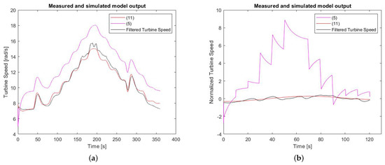
Figure 9. 2nd order model responses: (a) $\frac{\Delta \omega }{\Delta v}\left(s\right)$; (b) $\frac{\Delta \omega }{\Delta R_c}\left(s\right)$.

Regarding the 3rd order models, the results are similar, with the new model’s output closer to the expected values, as seen in Figure 10.

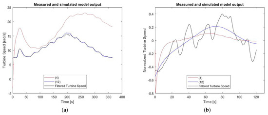
Figure 10. 3rd order model responses: (a) $\frac{\Delta \omega }{\Delta v}\left(s\right)$; (b) $\frac{\Delta \omega }{\Delta R_c}\left(s\right)$.

These results are confirmed in Table 5 where the performance index RMSD, given by (2), is calculated through a simulation resorting to Simulink. It must be mentioned that the simulation results could not perfectly replicate the signals given by the system identification toolbox; thus, the fit range is also mentioned, as it is a performance index calculated by the toolbox, and these results also confirm the results given by RMSD.

Table 5. Model comparison results.

Results
3rd Order Model						2nd Order Model
v(s)			$R_c\left(s\right)$			$v\left(s\right)$			$R_c\left(s\right)$
Equation	RMSD	Fit Value	Equation	RMSD	Fit Value	Equation	RMSD	Fit Value	Equation	RMSD	Fit Value
(4)	$76.92$	$-187.7$	(4)	$0.06$	$25.06$	(5)	$5.27$	$12.58$	(5)	$14.56$	$-1606$
(12)	$0.77$	$92.82$	(12)	$0.07$	$45.63$	(11)	$0.24$	$86.26$	(11)	$0.05$	$42.54$

Because the new models have a far better performance, new controllers were developed resorting to PID, LQR and CRONE methods, to replace those developed for the models in [17], that had been tested in simulation. As the performance of the 3rd order model exceeds that of the 2nd order model, without significant additional complexity in calculations, only the former model was used for control development.

3.3. Control Development

The proposed control objectives are the same as in [17], namely:

• Maximum overshoot of $20\%$ ($M_p\le 0.2$);
• Maximum settling time of 10 s ($t_s[2\%]\le 10$ s);
• Constant value for the tip speed ratio (TSR), $\lambda =0.2353$, which is the value imposed as optimal in [18].

3.3.1. PID Controller

The transfer function (TF) of the controller is given by:

$$G_c\left(s\right)=P+I\frac{1}{s}+D\frac{N}{1+N\frac{1}{s}},$$

(13)

where parameters

$$P_3=19928.885I_3=3566.699D_3=3918.396N_3=3.702,$$

(14)

were provided by Matlab R2020a’s PID Tuner application [23], according to the desired response’s specifications imposed by the user, set to a response time of $1.97$ s and a damping coefficient value of $0.9$.

Introducing these values into the PID block on the Simulink file and imposing a step signal as an input, the obtained results are seen in Figure 11, and the system’s characteristics are:

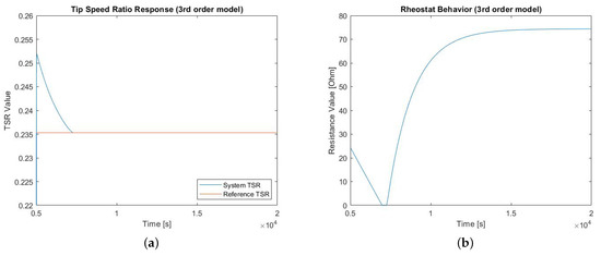
Figure 11. 3rd order model with PID response: (a) TSR response; (b) rheostat behavior.

• Maximum overshoot $M_p=7.0473\%$
• Settling time $t_s$($2\%$)$=1253.5$ s;
• Settling time $t_s$($5\%$)$=427.38$ s.

3.3.2. LQR Controller

The LQR controller minimizes a performance index J given by

$$\begin{array}{c}\hfill J={\int }_0^{+\infty }\left({\mathbf{x}}^{*}\mathbf{Q}\mathbf{x}+{\mathbf{u}}^{*}\mathbf{u}\right)\mathrm{d}t\end{array}$$

(15)

where $\mathbf{x}$ is the state vector of the state-space representation of the plant, $\mathbf{u}$ is the input vector, and $\mathbf{Q}$ is a matrix determining the relative weight of $\mathbf{x}$ and $\mathbf{u}$ in the minimization. Several values for Q were used, but the results turned out to be systematically worse than those of PID’s, with controllers not providing acceptable values of settling time and overshoot, and struggling instead to achieve the desired TSR value. Table 6 presents several examples and the system’s characteristics when applied in simulation.

Table 6. Results from developed LQR controllers for the 3rd order model.

			With Saturations
Q	${\mathit{k}}_{\mathit{r}}$	K	${\mathit{M}}_{\mathit{p}}$$[\%]$	${\mathit{t}}_{\mathit{s}}$ (5%) [s]	${\mathit{t}}_{\mathit{s}}$ (2%) [s]
$\left[\begin{array}{ccc}1& 0& 0\\ 0& 1& 0\\ 0& 0& 1\end{array}\right]$	$5\times {10}^6$	$\left[\begin{array}{ccc}2.3088& 2.4076& 0.99974\end{array}\right]$	$8.2068$	$553.17$	$6255.5$
$\left[\begin{array}{ccc}100& 0& 0\\ 0& 1& 0\\ 0& 0& 1\end{array}\right]$	$5\times {10}^6$	$\left[\begin{array}{ccc}10.353& 4.675& 0.99974\end{array}\right]$	-	-	-
$\left[\begin{array}{ccc}1& 0& 0\\ 0& 100& 0\\ 0& 0& 1\end{array}\right]$	$5\times {10}^6$	$\left[\begin{array}{ccc}4.5762& 10.451& 0.99974\end{array}\right]$	-	-	-
$\left[\begin{array}{ccc}1& 0& 0\\ 0& 1& 0\\ 0& 0& 100\end{array}\right]$	$5\times {10}^7$	$\left[\begin{array}{ccc}4.3698& 9.5066& 9.9997\end{array}\right]$	$6.5346$	$616.26$	-

3.3.3. CRONE Controller

There are three generations of CRONE controllers (from the French acronym Commande Robuste d’Ordre Non-Entier), having in common that the justification of their design is based upon fractional derivatives [24,25]. The resulting controller, however, has a TF that only resorts to integer order derivatives, i.e., a TF, which is a rational function in s. Third generation CRONE controllers are used when the model of a plant is known with uncertainty, as is the case of the wind turbine [26]. The purpose of the controller is to ensure a desired behavior for the nominal plant, and minimize performance changes if model parameters vary within the expected ranges of uncertainty. For the development of this controller, a Matlab toolbox created by the CRONE Research Group of Université de Bordeaux was used.

To develop this type of controller, extreme plants must be defined, corresponding to the maximum effects of uncertainty in the model. For that purpose, two types of uncertainties were considered, parametric and pole/zero location. Through the calculation of NRMSD, given by (3), it was found that the parametric uncertainty possessed better results, as the corresponding dispersion was more localized, and the resulting controller more robust. The extreme plants are given by:

$$\begin{array}{c}\hfill {G_3}^{\mathtt{l}}\left(s\right)=\frac{4.107\times {10}^{-5}{s}^2+4.686\times {10}^{-6}s+1.7\times {10}^{-7}}{s^3+0.08925s^2+0.00543s+0.0002229},\\ \hfill \end{array}$$

(16)

$$\begin{array}{c}\hfill {G_3}^{\mathtt{u}}\left(s\right)=\frac{5.557\times {10}^{-5}{s}^2+6.34\times {10}^{-6}s+2.3\times {10}^{-7}}{s^3+0.1207s^2+0.007346s+0.0003015},\end{array}$$

(17)

corresponding to the lower and upper bound extreme plants, respectively.

With the nominal and extreme plants determined, the toolbox can be used to develop CRONE controllers, with the choice of desired specifications introduced by the user [27]. The developed controllers are presented in Table 7, where the value of “Desired $t_s$” is chosen by the user and defines the settling time $t_s$ [5%].

Table 7. Results from the developed CRONE controllers.

	3rd Order Model
Theoretical ${\mathit{t}}_{\mathit{s}}$		${\mathit{t}}_{\mathit{s}}$ (5%) [s]	${\mathit{t}}_{\mathit{s}}$ (2%) [s]	${\mathit{M}}_{\mathit{p}}$ [%]
5		$1013.1$	2307	$10.3$
10		$1273.9$	2856	$11.3$
50		$1054.4$	$2389.7$	$10.5$
70		$817.9$	$1934.2$	$9.3$
90		$595.0$	$1540.9$	$8.0$
100		$539.4$	$1447.5$	$7.7$
200		$713.2$	$1745.4$	$8.7$
300		$572.6$	$1503.1$	$7.9$
400		$514.5$	$1406.3$	$7.5$
500		$485.3$	$1358.3$	$7.3$
600		$465.2$	$1325.5$	$7.2$
700		459	$1315.4$	$7.2$
800		$492.8$	$1370.5$	$7.3$
900		$502.0$	$1385.6$	$7.3$
1000		$477.3$	$1345.2$	$7.2$

The results show a significant discrepancy between the desired and the actual settling time, which may be due to the incapacity of the plant to respond as fast as desired, when the specification $t_s$ is low. Taking into account the results obtained, the chosen CRONE controller is the one with $t_s$ set for 700 s, given by:

$$G_c\left(s\right)=\frac{1.194}{s+0.07361}+\frac{-9.733}{s+0.005829}+\frac{9.55}{s}.$$

(18)

The corresponding response can be seen in Figure 12.

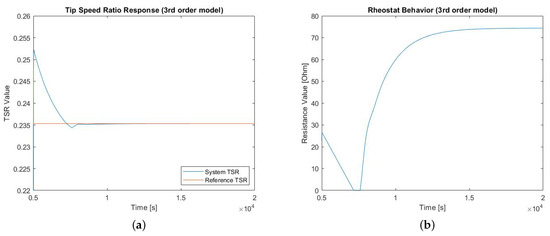
Figure 12. 3rd order model with CRONE response: (a) TSR response; (b) rheostat behavior.

3.4. Controller’s Performance Comparison

From the responses for an input signal in the form of a step, with the characteristics given by Table 8, it is clear that the LQR controller possesses the worst performance; as such it will be omitted from other input signals [28].

Table 8. Controller’s performance for a step signal input.

Model	${\mathit{M}}_{\mathit{p}}$ [%]	${\mathit{t}}_{\mathit{s}}$ (5%) [s]	${\mathit{t}}_{\mathit{s}}$ (2%) [s]
PID	$7.0473$	$427.38$	$1253.5$
LQR	$8.2068$	$553.17$	$6255.5$
CRONE	$7.1681$	459	$1315.4$

Changing the input signal from a step signal to a ramp with slope $1/120$, in order to simulate a unitary increase in wind velocity in 2 minutes, the results are as shown in Figure 13. In order to simulate a real input signal, the last input signal is corrupted with additive white noise, and the results become those in Figure 14.

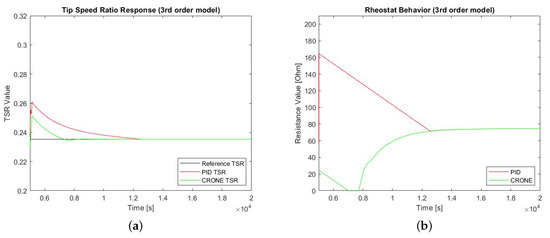
Figure 13. Controller comparison with ramp signal: (a) TSR response; and (b) rheostat behavior.

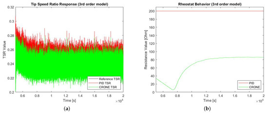
Figure 14. Controller comparison with noise corrupted ramp signal: (a) TSR response; and (b) rheostat behavior.

As can be observed, the PID controller has a poorer response for ramp signals, whether corrupted with noise or not, whilst the CRONE controller maintains the rheostat’s behavior. Thus, this was the controller chosen for implementation.

3.5. System Discretization

The chosen method of discretization was Tustin’s, in order to preserve stability in conversion (which is not ensured by simpler methods, like rectangular approximations), and decrease the resulting bias due to the discretization. For the purpose of choosing a sample time value, its effect on the controller’s behavior was studied, with the results presented in Figure 15.

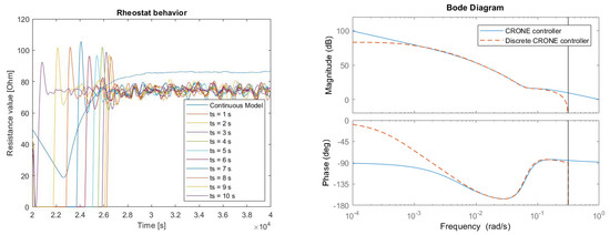
Figure 15. Effect of the sampling time on the rheostat’s behavior. Left: time response; Right: frequency response.

A sampling time of $t_s=10$ s is seen to include the bandwidth of the controller. Time response simulations show that the overshoot and settling time of the rheostat would be more significant with lower sampling times, so there is no advantage in choosing a shorter sample time. As such, that value of the sampling time was chosen, resulting in discrete TFs given by:

$$\begin{array}{c}\hfill \Delta \omega \left(z\right)=\frac{1.489z^3+1.677z^2-1.113z-1.301}{z^3+1.079z^2-0.7175z-0.7969}\Delta v\left(z\right)+\\ \hfill \\ \hfill +\frac{0.00026z^3+3.02\times {10}^{-6}{z}^2-0.0001814z+7.557\times {10}^{-5}}{z^3-1.758z^2+1.269z-0.3047}\Delta R_c\left(z\right),\end{array}$$

(19)

$$G_c\left(z\right)=\frac{4.826z^3-1.626z^2-3.371z+3.081}{z^3-2.405z^2+1.841z-0.4358},$$

(20)

which were then applied by the Arduino.

3.6. Controller Testing

In order to test the controller, a control problem must be defined first. For that purpose, the system’s overall TSR is studied, which is given by the following equation:

$$TSR=\frac{{\omega }_{v}r}{v}+\frac{{\omega }_{R_c}r}{v},$$

(21)

where $r=0.173$ m, defining the radius of the turbine, v is the wind velocity intensity, and $\omega$ defines the turbine’s angular velocity from each term, v or resistance $R_c$. Through simulation results, the system’s minimum and maximum TSR values were found, as functions of the wind velocity, as presented by Figure 16, which also shows the expected actuation range of the wind tunnel.

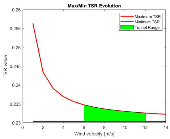
Figure 16. System’s TSR as function of v.

As the maximum TSR distribution is significantly different from the minimum distribution, it was decided to set the reference value as the system’s TSR mean value in order to impose a reaction from the controller with either an increase or decrease in wind velocity intensity.

The results of the tests in the wind tunnel are presented in Figure 17, and compared with simulation results, for the same wind velocity input signal, in Figure 18.

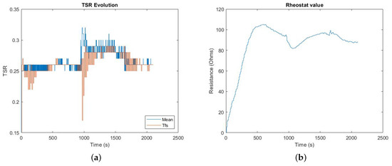
Figure 17. Results from the controller’s implementation in the wind tunnel: (a) TSR response; and (b) rheostat behavior.

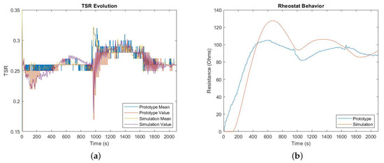
Figure 18. Results from the controller’s implementation in the wind tunnel: (a) TSR response; and (b) rheostat behavior.

From Figure 17, there are two instances of interest: the first occurring around t$\approx 900$ s and the second at about t$\approx 1750$ s. These instances correspond to a decrease and an increase in the perceived wind velocity intensity by the anemometer, respectively, which prove that the controller works as intended.

For instance, for a decrease in the perceived wind velocity intensity, the mean TSR is increased, but due to the delay caused by the discrete TF’s sampling time, the reference TSR is still the prior to the change of wind velocity, which is now lower than the desired TSR. Thus, the controller lowers the rheostat’s value, corresponding to the sudden fall visible at t$\approx 900$ s in Figure 17b. The same occurs for an increase of wind velocity intensity, with a sudden increase in the rheostat’s value seen at t$\approx 1750$ s.

Comparing the results in the simulation from the results obtained in the wind tunnel, it can be observed, from Figure 18, that the results of simulation are worse than the results from the actual controller’s implementation, with higher overshoot and settling time. This may be due to a faster implementation of the algorithm in the Arduino, when compared to the numerical approximation used by Simulink.

4. Conclusions

With this work, the technology readiness level is increased to 4. Although the controller’s implementation is considered a success, even surpassing the expected performance shown by simulation results, it might be further improved. For instance, with the presence of a reliable controller and some programming, it is now possible to obtain dedicated data sets for the second term of the prototype, i.e., the term of $\frac{\Delta \omega }{\Delta R_c}\left(s\right)$, instead of using the manipulated data.

Other minor improvements are also possible to occur with simple maintenance of the turbine, such as the repair of superficial flaws of the blades, correct alignment of the blades and the correct alignment of the generator’s rotational axis.

References

- IEA. Renewables Information: Overview; IEA: Paris, France, 2020. [Google Scholar]
- Batista, N.C.; Melicio, R.; Mendes, V.M.F.; Calderón, M.; Ramiro, A. On a Self Start Darrieus Wind Turbine; Blade Design and Field Tests. Renew. Sustain. Energy Rev. 2015, 5, 508–522. [Google Scholar] [CrossRef]
- Muller, G.; Jentsch, M.F.; Stoddart, E. Vertical Axis Resistance Type Wind Turbines for use in Buildings. Renew. Energy 2009, 34, 1407–1412. [Google Scholar] [CrossRef]
- Balduzzi, F.; Bianchini, A.; Carnevale, E.A.; Ferrari, L. Feasibility Analysis of a Darrieus Vertical Axis Wind Turbine Installation in the Rooftop of a Building. Renew. Energy 2012, 97, 921–929. [Google Scholar] [CrossRef]
- Tiju, W.; Marnoto, T.; Sohif, M.; Ruslan, M.H. Darrieus Vertical Axis Wind Turbine for Power Generation I: Assessment of Darrieus VAWT Configurations. Renew. Energy 2015, 75, 50–67. [Google Scholar] [CrossRef]
- Batista, N.C.; Melicio, R.; Matias, J.C.O.; Catalão, J.P.S. Self-start performance evaluation in Darrieus-type vertical axis wind turbines: Methodology and computational tool applied to symmetrical airfoils. Renew. Energy Power Qual. J. 2011, 1, 250–255. [Google Scholar] [CrossRef]
- Batista, N.C.; Melicio, R.; Matias, J.; Catalão, J.P.S. Self-start Evaluation in lift-type vertical axis wind turbines: Methodology and computational tool applied to asymmetrical airfoils. In Proceedings of the International Conference on Power Engineering, Energy and Electrical Drives, Malaga, Spain, 11–13 May 2011; pp. 1–6. [Google Scholar]
- Alam, M.J.; Iqbal, M.T. Design and Development of hybrid Vertical Axis Turbine. In Proceedings of the 2009 Canadian Conference on Electrical and Computer Engineering, St. John’s, NL, Canada, 3–6 May 2009; pp. 1178–1183. [Google Scholar]
- Matias, J.; Batista, N.C.; Melicio, R.; Catalão, J.P.S. Vertical Axis Wind Turbine performance prediction: An approach to the double multiple streamtube model. In Proceedings of the International Conference on Renewable Energies and Power Quality, Santiago de Compostela, Spain, 28–30 March 2012. [Google Scholar]
- Chong, W.T.; Poh, S.C.; Fazlizan, A.; Pan, K. Vertical Axis Wind Turbine with Omni-directional-guide-vane for Urban High-rise Buildings. J. Cent. South Univ. 2012, 19, 727–732. [Google Scholar] [CrossRef]
- Grant, A.; Johnstone, C.; Kelly, N. The potential of ducted turbines. Renew. Energy 2008, 33, 1157–1163. [Google Scholar] [CrossRef]
- Andriollo, M.; Bortoli, M.D.; Martinelli, G.; Morini, A.; Tortella, A. Control strategies fora VAWT driven pm synchronous generator. In Proceedings of the International Symposium on Power Electronics, Electrical Drives, Automation and Motion, Ischia, Italy, 11–13 June 2008; pp. 804–809. [Google Scholar]
- Melicio, R.; Mendes, V.M.F.; Catalão, J.P.S. Fractional-order control and simulation of wind energy systems with pmsg/full-power converter topology. Energy Convers. Manag. 2010, 51, 1250–1258. [Google Scholar] [CrossRef]
- Melicio, R.; Mendes, V.M.F.; Catalão, J.P.S. Two-level and Multilevel Converters for Wind Energy Systems: A Comparative Study. In Proceedings of the 13th International Power Electronics and Motion Control Conference—EPE-PEMC 2008, Poznań, Poland, 1–3 September 2008; pp. 1682–1687. [Google Scholar]
- Melicio, R.; Mendes, V.M.F.; Catalão, J.P.S. A Pitch Control Malfunction Analysis for Wind Turbines with Permanent Magnet Synchronous Generator and Full-power Converters: Proportional Integral Versus Fractional-order Controllers. Electr. Power Compon. Syst. 2010, 38, 387–406. [Google Scholar] [CrossRef]
- Batista, N.C.; Melicio, R.; Mendes, V.M.F. Darrieus-type vertical axis rotary-wings with a new design approach grounded in double-multiple streamtube performance prediction model. AIMS Energy 2018, 6, 673–694. [Google Scholar] [CrossRef]
- Pereira, T.R.; Batista, N.C.; Fonseca, A.R.A.; Cardeira, C.; Oliveira, P.; Melicio, R. Darrieus wind turbine prototype: Dynamic modeling parameter identification and control analysis. Energy 2018, 159, 961–976. [Google Scholar] [CrossRef]
- Ravasco, F.; Melicio, R.; Batista, N.C.; Valério, D. A wind turbine and its robust control using the CRONE method. Renew. Energy 2020, 160, 483–497. [Google Scholar] [CrossRef]
- Fialho, L.; Melicio, R.; Mendes, V.M.F.; Figueiredo, J.; Collares-Pereira, M. Effect of Shading on Series Solar Modules: Simulation and Experimental Results. Procedia Technol. 2014, 17, 295–302. [Google Scholar] [CrossRef]
- Weather Meter Hookup Guide. Available online: https://learn.sparkfun.com/tutorials/weather-meter-hookup-guide/all (accessed on 8 February 2022).
- Mathworks Help Center. Available online: https://www.mathworks.com/help/ident/gs/about-system-identification.html (accessed on 12 October 2021).
- PTRobotics Site. Available online: https://www.ptrobotics.com/servomotor/7879-servo-towerpro-mg995-servo-270.html (accessed on 21 July 2022).
- Mathworks Help Center. Available online: https://www.mathworks.com/help/control/getstart/pid-controller-design-for-fast-reference-tracking.html (accessed on 28 May 2022).
- Sabatier, J.; Lanusse, P.; Melchior, P.; Oustaloup, A. Fractional Order Differentiation and Robust Control Design: CRONE, H-Infinity and Motion Control; Springer: Berlin/Heidelberg, Germany, 2015. [Google Scholar]
- Valério, D.; Sá da Costa, J. An Introduction to Fractional Control; IET: Stevenage, UK, 2013. [Google Scholar]
- Oustaloup, A.; Levron, F.; Matthieu, B.; Nanot, F.M. Frequency-band complex noninteger differentiator: Characterization and synthesis. IEEE Trans. Circuits Syst. Fundam. Theory Appl. 2000, 47, 25–39. [Google Scholar] [CrossRef]
- CRONE Group. CRONE Control Design Module User’s Guide; Université de Bordeaux: Bordeaux, France, 2010. [Google Scholar]
- Rodrigues, G.; Melicio, R.; Valério, D. Experimental validation of a wind turbine. In Proceedings of the IEEE International Conference on Control, Automation and Diagnosis (ICCAD’22), Lisbon, Portugal, 1–6 July 2022. [Google Scholar]
Publisher’s Note: MDPI stays neutral with regard to jurisdictional claims in published maps and institutional affiliations. |
© 2022 by the authors. Licensee MDPI, Basel, Switzerland. This article is an open access article distributed under the terms and conditions of the Creative Commons Attribution (CC BY) license (https://creativecommons.org/licenses/by/4.0/).