A Machine Learning Method for the Risk Prediction of Casing Damage and Its Application in Waterflooding

Abstract

During the development of oilfields, casings in long-term service tend to be damaged to different degrees, leading to poor development of the oilfields, ineffective water circulation, and wasted water resources. In this paper, we propose a data-based method for predicting casing failure risk at both well and well-layer granularity and illustrate the application of the method to GX Block in an eastern oilfield of China. We first quantify the main control factors of casing damage by adopting the F-test and mutual information, such as that of the completion days, oil rate, and wall thickness. We then select the top 30 factors to construct the probability prediction model separately using seven algorithms, namely the decision tree, random forest, AdaBoost, gradient boosting decision tree, XGBoost, LightGBM, and backpropagation neural network algorithms. In terms of five evaluation indicators, namely the accuracy, precision, recall, F1-score, and area under the curve, we find that the LightGBM algorithm yields the best results at both granularities. The accuracy of the prediction model based on the preferred algorithm reaches 87.29% and 92.45% at well and well-layer granularity, respectively.

1. Introduction

As a waterflooding program deepens, the well casing that has been in service for a long time is damaged to varying degrees, mainly through deformation, rupture, and seal failure. Casing damage is a global problem that needs to be solved urgently. Casing damage has occurred in oilfields around the world, and there has been an alarming rate of casing failure of up to 50%, which has not been widely reported for reasons relating to reputation, company profiles, and privacy [1]. Wells in China have suffered serious casing damage. Oilfields in China are mainly clastic sandstone reservoirs with low natural energy. Water flooding is the main method used to develop China’s oilfields, adopted for 82% of the country’s developed reserves. By 2021, the casing damage rate of all major oilfields in China had exceeded 20%, the rate at oilfields such as Huabei, Shengli, and Jianghan had exceeded 30%, and the rate even exceeded 50% in some regions [2]. The occurrence of casing-damaged wells has caused problems such as imperfect well groups, unbalanced injection and production, and ineffective circulation of water. Casing damage cannot be ignored for oilfields developed through separate-layer waterflooding. If the damage point is outside the oil formation, the injected water will enter the layers without an injection-production well pattern, resulting in a great waste of water resources. If the damage point is inside the oil formation, the injection is equivalent to general instead of zonal injection, resulting in ineffective water circulation. In China, water consumption per ton of oil increased from 4.9 cubic meters in 1991 to 12 cubic meters in 2019. Therefore, the prediction, detection, and treatment of casing damage have long been a technical hotspot in oilfield development.

Casing damage is a complex problem. Scholars have carried out a series of studies on the mechanism, influencing factors, evaluation, and prediction of casing-damaged wells [3].

Studies on the causes and influencing factors of casing damage have mostly been carried out from qualitative and mechanical points of view or by establishing comprehensive evaluation indicators for parameters [4,5,6,7,8]. In general, casing damage is comprehensively affected by various elements, which can be roughly divided into geology, development, engineering, corrosion, and other factors [9,10,11,12,13,14]. The various factors of casing damage have nonlinear, uncertain, and time-varying characteristics [3].

The traditional approach to evaluating and predicting casing damage has been to establish a mechanical model and analyze the quantitative conditions of casing damage by studying the degrees of influence of various factors. There are three main types of methods, namely analytical methods, numerical analysis methods, and measurement methods. The first kind of method assumes that the casing is an ideal circle, and the damage is predicted by analyzing the deformation characteristics of the casing under a nonuniform external load. The second kind of method is based on finite element theory and uses commercial software to establish a spatial simulation mechanical model with which to simulate the casing deformation under the combined load of compression, torsion, and bending and to analyze the stress and deformation characteristics of the oil and water well casing through numerical calculation. Examples of this type of method are the finite element method, boundary element method presented by Lian [15,16], Lagrange element method presented by Deng [17], and coupled seepage–geomechanics models represented by Han [18]. The third kind of method effectively identifies casing damage and quantitatively evaluates the casing health through measurement of the water injection profile, pulsed neutron analysis, measurement of the multi-arm well diameter, acoustic logging, and electromagnetic flaw detection [19,20,21,22]. These prediction methods are usually limited by the ambiguity of evaluation criteria and difficulty of quantitative assessment. Zhang et al. thus proposed a fuzzy comprehensive evaluation and prediction model based on the analytic hierarchy process to determine the weights of factors and quantitatively analyze casing damage [13]. Wang et al. proposed a matrix-based casing damage assessment method for hydraulic fracturing based on quantitative risk analysis [23].

Traditional methods clarify the geological and external conditions that cause casing damage but face multiple problems. First, the analytical method assumes ideal conditions, which do not fully represent the actual well conditions. Second, neither the analytical method nor the numerical analysis method is suited to considering the comprehensive effect of multiple factors in establishing the model. Third, although the measurement method can effectively confirm the casing damage of a single well, its operational process is complex and high-risk, and it can only identify whether the casing failure has occurred and does not make a prediction of failure in advance. Therefore, the conventional methods have certain limitations and are not suited to predicting the probability of casing damage that may occur in the future.

With the rapid development of information technologies such as big data and artificial intelligence, intelligent data-driven prediction and analysis of casing failure have been reported, but such research is still in its infancy. The basic idea of a data-driven identification and intelligent prediction method for casing damage is to use algorithms related to feature engineering in selecting influencing factors and establishing a mathematical model to describe and predict the probability of casing failure. Representative data-driven methods are the use of a support vector machine (SVM) or neural network and other bagging and boosting machine learning methods. The casing-damage prediction method of the SVM takes the influencing factors of casing damage as the input of the SVM and optimizes the parameters of the SVM using an immune algorithm to make an accurate prediction. The use of SVM algorithms to build single-well casing loss prediction models has been shown to achieve good results [16,24,25,26,27]. Additionally, the artificial neural network has attracted much attention for its strong autonomous learning, strong memory and fault tolerance, strong nonlinear parallel processing ability, and other characteristics. Neural networks, and especially the backpropagation neural network, have gradually been applied in the prediction of casing damage [3,28,29]. Given the risk of overfitting in a complex neural network, Wang et al. used the Bayesian neural network of the hybrid Monte Carlo algorithm to predict casing damage. This method has higher prediction accuracy and stronger generalization ability than the binarized neural network algorithm of the backpropagation neural network and the Laplace algorithm [30].

As the oil industry enters the era of big data, scholars are continually attempting to use a variety of bagging and boosting algorithms to improve the accuracy of casing damage prediction. Zhou and Li applied the gradient boosting decision tree (GBDT) algorithm to build a casing damage assessment model for predicting the possibility and probability of well casing failure and obtained prediction results that were in line with actual observations [25]. Noshi et al. used a data-driven method to identify the characteristics of casing damage during drilling and fracturing and found the gradient boosting machine to perform best in a comparison of nine machine-learning algorithms [31]. They then built a prediction model using an artificial neural network and boosted ensemble trees considering 26 features from drilling, fracturing, and geological data [32]. Song and Zhou selected 10 parameters that had the greatest effects on casing damage through principal component analysis and established a prediction model based on the GBDT algorithm. Experiment results showed that their approach had 86.3% precision [33]. Tang et al. proposed a prediction model based on LightGBM and XGBoost algorithms considering 19 main control factors [34]. Tan et al. established data-driven casing damage prediction models for oil production wells based on XGBoost and LightGBM machine-learning algorithms, considering the factors of dynamic production, and they compared the prediction performances of the two models [35]. Carpenter et al. established a data-driven casing damage prediction model using boosted-ensemble trees and artificial neural network algorithms based on data visualization by a box mosaic plot and trellis chart [36]. Xue et al. established a classification method based on a random forest (RF) algorithm to predict the casing damage classification. Experimental results showed that the prediction accuracy of their method was 95% [37]. Li et al. compared the performance of several classification models commonly used in casing damage prediction and proposed an improved AdaBoost algorithm for the uneven distribution of casing damage samples, which effectively improved the prediction accuracy [38]. Noshi and Amani developed a data-driven tool that applies several statistical methods to naturally alleviate the casing failure risk. They not only proposed a methodology but also formed the basis of a new casing risk assessment criterion [1]. Additionally, they proposed a data-driven alternative that takes as input the active and passive factors and outputs the corresponding total local strain that reflects the effects to estimate the fatigue life of a casing [39].

Undoubtedly, with the development of data science, machine learning technology has provided new ideas and methods for casing damage prediction. However, there remain several problems in the current research. First, the data often determine the precision of the machine learning model, and the complexity and low availability of actual oilfield data make the creation of a data set for an intelligent prediction model challenging. Additionally, when choosing different input parameters, the model accuracy varies greatly, even when predictions are made with identical algorithms. Casing damage is affected by factors that are nonlinear, uncertain, and time varying. The above studies established prediction models based on static data, such as data on geological and engineering parameters, ignoring production data. A few scholars have considered dynamic data, but they converted these data into static data by taking extreme values, mean values, variances, and other statistical values, thus losing the time-sequence features. Finally, previous casing damage predictions have often been made for a single well and do not clarify the specific casing damage layer.

Against the above research background, this paper proposes a model for predicting the casing damage risk based on machine learning. The paper starts with the determination of the main control factors by adopting box plots, F-tests, and mutual information. To further clarify the specific casing damage layer, the paper puts forward two processing schemes with different data granularities, namely well and well-layer granularities. Moreover, seven algorithms, namely the decision tree (DT), RF, AdaBoost, GBDT, extreme gradient boosting (XGBoost), light gradient boosting machine (LightGBM), and backpropagation neural network algorithms, are used to build the probability prediction model. The accuracy of each model is evaluated using five evaluation indices, namely the accuracy, precision, recall, F1-score, and area under the curve (AUC). Finally, the optimal model is obtained in terms of the errors. Model verification using actual sample data for GX Block in an eastern China oilfield shows that the prediction accuracy of LightGBM model is the highest. Using this model and the dynamic and static data of wells, the risk of casing damage can be identified, and effective preventive measures can be taken in advance, which will reduce the probability of damage to the casings of oil and water wells, prolong the life cycles of the casings, and improve the effectiveness of oilfield development and economic benefits.

The remainder of the paper is organized as follows. Section 2 presents the concepts and methods adopted in the paper to construct predictive models using seven intelligent algorithms. Section 3 presents a case study of applying the above methodology to GX Block. Section 4 outlines the constraints of this research. Finally, Section 5 summarizes the main findings of the paper.

2. Methodology

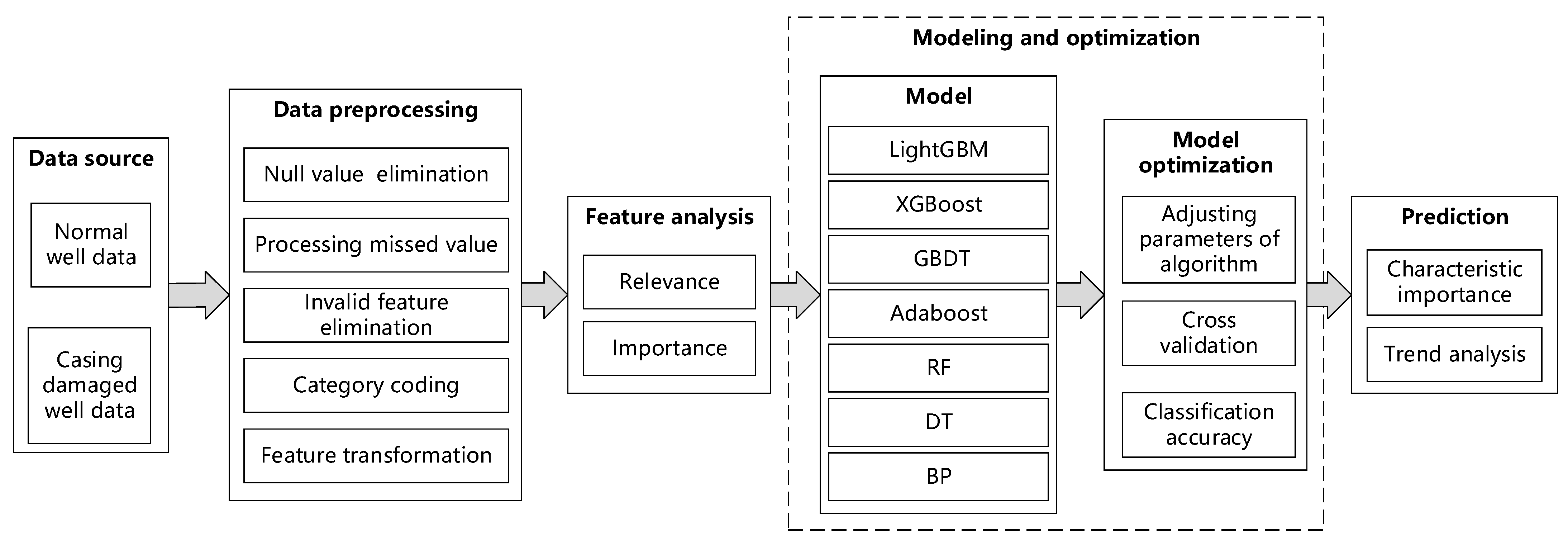
2.1. Technical Concept

Multiple intelligent algorithms were adopted to construct an intelligent predictive model of casing damage using geology, engineering, development, and production data through the quantitative identification of the main controlling factors. The workflow comprises five steps, as described below and shown in Figure 1.

(1)

Collect data for normal and casing-damaged wells, such as sublayer data, perforation data, casing data, and production data.

(2)

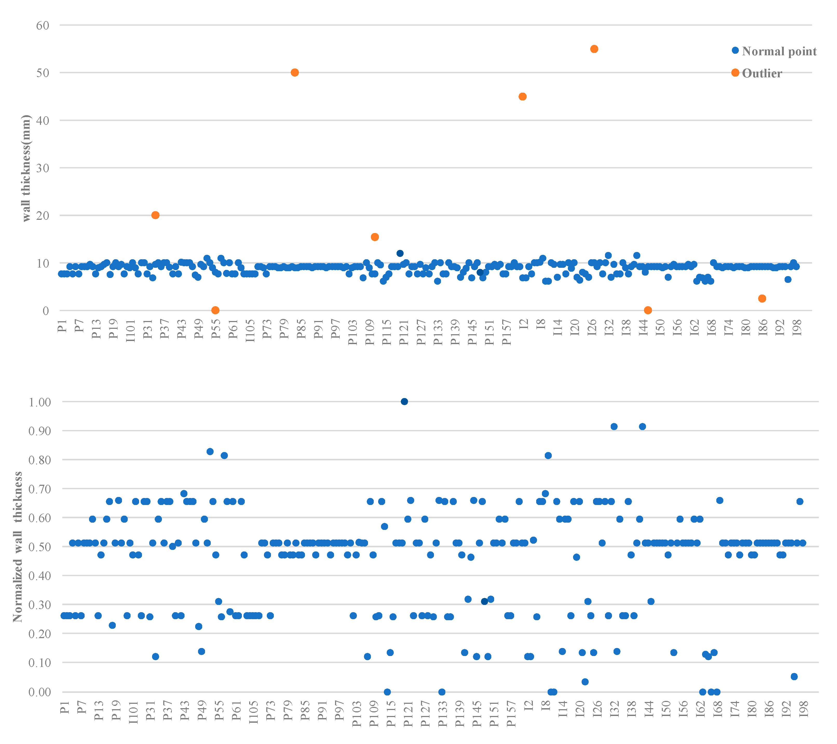
Preprocess the collected data through null-value elimination, missed-value processing, invalid-feature elimination, and category coding. Aggregate and construct new parameters based on the original data, and preliminarily determine the data items having a strong correlation with casing damage.

(3)

Adopt a box plot, F-test, and mutual information, among other methods, to analyze the correlation between factor characteristics and casing damage.

(4)

Use seven common machine learning classification algorithms to build the casing damage prediction model and adjust the main parameters of the algorithms. Then verify the model adopting five-fold cross-validation. Evaluate the accuracy of the model using five indicators, namely the accuracy, precision, recall, F1-score, and AUC. Finally, obtain the optimal model in terms of these errors.

(5)

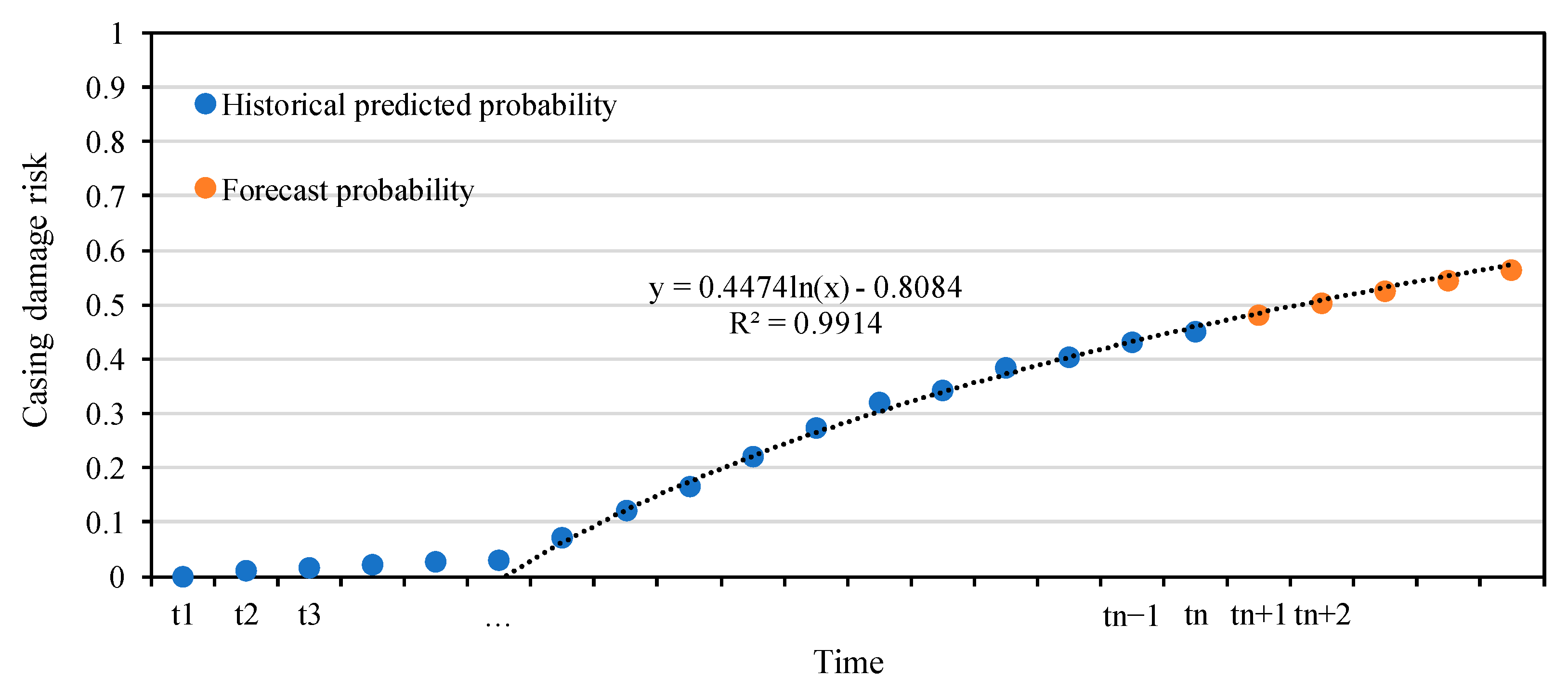
Apply the optimal model to predict the probability of casing damage in wells.

To further identify the layer with casing damage, two schemes based on well and well-layer granularities are proposed. The two schemes share the same workflow but rely on different data sources, see

Table 1. Comparison of the modeling schemes of two granularities.

Scheme	Function	Database	Advantage	Disadvantage
Well granularity	Predict casing damage for a single well	Single well data	Easy to prepare data	Geological layer, perforation, and other related data need to be aggregated upward, resulting in information loss
Well-layer granularity	Predict casing damage for each well layer	Sub-layer data	Fully use of geology and engineering layer information	Difficult to prepare data, and the production data of sub-layers often needs to be obtained by other technical means

.

The well-granularity scheme builds a model using the data of the whole well and predicts the casing status of a single well. The data used are relatively coarse and easy to prepare, but the statistical characteristics used for prediction, such as formation and perforation, require upward aggregation, which results in information loss. Moreover, the casing damage can only be located to the well and not to the specific layer. This scheme is suitable for modeling in the case of incomplete sub-layer data.

The well-layer granularity scheme uses well-layer data to build a model and predicts the casing status of a specific layer for each well. It fully uses the layer geological and engineering information and accurately locates the layer where casing damage may occur. However, it requires sub-layer production data that are often obtained by other technical means, and it is thus difficult to prepare the data. This scheme is suitable for modeling in the case of a large sample data volume and finer data granularity.

2.2. Feature Analysis

The analysis of relevant features before modeling reduces the risk of overfitting, improves the training speed, reduces the operation cost, and improves the accuracy of the model. The selection of features having the strongest correlation with the fitting target often achieves twice the result with half the effort. The establishment of the intelligent prediction model for the casing status first involves an investigation of the causes of casing damage, then sorts out the corresponding influencing factors, and finally abstracts the actual engineering problems into mathematical models.

The correlation analysis is conducted on the sample data using the following methods.

(1)

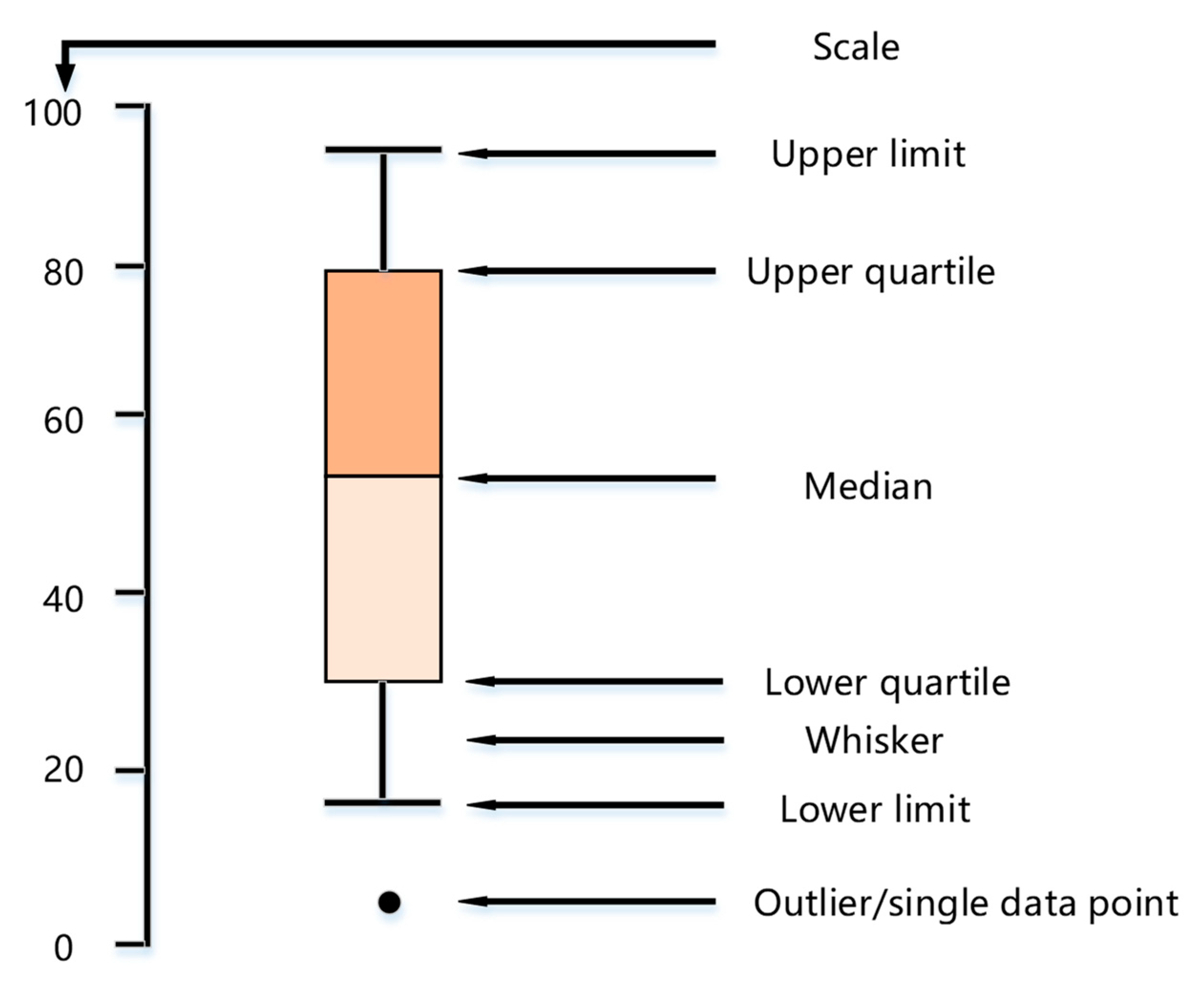
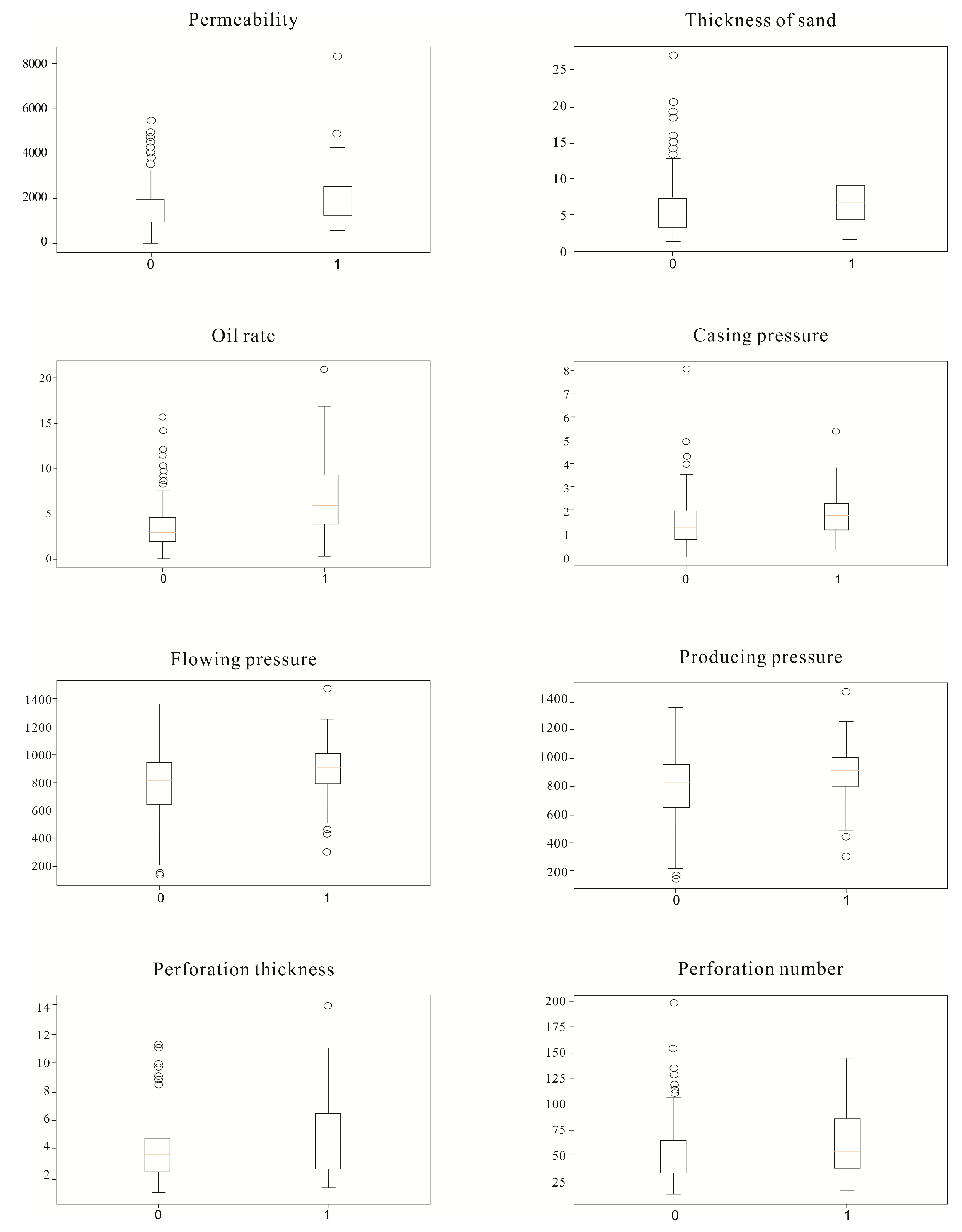
Box-plot visualization: A data distribution can be visualized using five statistical values of the data, namely the minimum, upper quartile, median, lower quartile, and maximum, as shown in Figure 2. This box-plot visualization is unaffected by outliers and shows whether the data are roughly symmetry, accurately and stably describes the discrete distribution of the data, especially for the comparison of several types of samples, and is conducive to data cleaning.

(2)

F-test: The F-test is a filtering method used to capture the linear relationship between each feature and label. The F-test is adopted to analyze the test data, test whether the average values of multiple normal populations with equal variances are equal and judge the importance of the effects of various factors on the test indicators.

The test statistic F is calculated as

$$F=\frac{SSA/df1}{SSE/df2}=\frac{{\sum }_{i=1}^r{\sum }_{j=1}^m{\left(y_{ij}-\overline{y_{i·}}\right)}^2/\left(n-r\right)}{{\sum }_{i=1}^{r}m{\left(\overline{y_{i·}}-\overline{y}\right)}^2/\left(r-1\right)},$$

(1)

where there is a total of n tests divided into r groups, with m times in each group. SSA (sum of squares between groups) is the sum of squares of deviations between various grades, and SSE (sum of square error) is the sum of squared errors within each grade. df1 is the freedom of SSA, and df2 is the freedom of SSE.

This study conducted F-test analysis to verify whether each feature has a significant effect on the casing-damaged label. The feature that the larger F value and the p value less than 0.05 has a significant effect on whether it is casing damaged labels.

(3)

Calculation of mutual information: Mutual information is an information measure used in information theory to estimate the correlation between category features and labels. Mutual information takes a non-negative value. Mutual information is equal to zero if and only if the two features are independent and have a higher value for higher dependency. Mutual information can be regarded as the amount of information about another random variable contained in one random variable or the decrease in uncertainty of a random variable due to knowing another random variable.

If random variables (X, Y) ~ P(X, Y), then the mutual information of X and Y is defined as

$$I\left(X;Y\right)={\displaystyle \sum }_{y\in Y}{\displaystyle \sum }_{x\in X}p\left(x,y\right)log(\frac{p\left(x,y\right)}{(p\left(x\right)p\left(y\right)}).$$

(2)

Mutual information can be easily converted in the form of KL divergence:

$$I\left(X;Y\right)={\displaystyle \sum }_{y\in Y}{\displaystyle \sum }_{x\in X}p\left(x,y\right)log\left(\frac{p\left(x,y\right)}{(p\left(x\right)p\left(y\right)}\right)=D_{KL}(p\left(x,y\right)||p\left(x\right)p\left(y\right)).$$

(3)

KL divergence can be used to measure the difference between two probability distributions. If x and y are independent random variables, then p(x, y) = p(x)p(y), and the above expression equals zero. Therefore, a larger I(X; Y) corresponds to a greater correlation between the two variables, such that mutual information can be used to filter features. Against the application background of feature selection, we hope that a smaller uncertainty in Y is better. This is more conducive to classification. Greater mutual information means that the uncertainty of Y is reduced more by feature X, i.e., more information about Y is contained in X. This paper measures the correlation between features and determines whether a casing damage label by calculating the mutual information.

2.3. Model Establishment

(1)

Modeling algorithms

As mentioned above, previous research has used three main types of methods for predicting casing damage, namely SVM, neural network, and other bagging and boosting machine learning methods. In comparing the prediction performance of different algorithms and selecting the most suitable modeling algorithm, seven common algorithms (DT, RF, AdaBoost, GBDT, XGBoost, LightGBM, and backpropagation neural network algorithms) from the latter two categories were used to establish the casing damage risk prediction model. The SVM was excluded from this study because it is an older classification algorithm based on linear segmentation. This study used Sklearn and Tensorflow for machine learning and deep learning, respectively, in training the models in Python.

(2)

Parameter optimization

In a machine learning model, the parameters that need to be manually selected are called super parameters. For example, the number of decision trees in the RF, the number of hidden layers and nodes in each layer of an artificial neural network, the size of the regular term coefficient, and other parameters need to be specified in advance. If the super parameters are not properly selected, there will be a problem of underfitting or overfitting. This study adopted a grid search to adjust the parameters and obtain the best combination.

(3)

Effect verification

Five-fold cross-validation was conducted to simultaneously traverse multiple parameters, classification thresholds, and feature combinations of the seven algorithms in optimizing the model. To reduce the prediction randomness of the model with an insufficient data sample size, multiple (e.g., 100 times or more) random 4:1 partitioning of the training and test sets can be performed.

(4)

Model accuracy evaluation

If our classification target has only two categories, recorded as positive and negative, the four counts are the numbers of true positives (TP), false positives (FP), false negatives (FN), and true negatives (TN). See

Table 2. Confusion matrix of the prediction results.

		Predicted Class
		Class = Casing Damaged Well	Class = Normal Well
Actual class	Class = casing damaged well	True positives (TP)	False negatives (FN)
	Class = normal well	False positives (FP)	True negatives (TN)

for the classification of the four counts.

The accuracy of the model was evaluated using five indicators (accuracy, precision, recall, F1-score, and AUC), as shown in

Table 3. Model accuracy evaluation indicators.

Evaluation Indicator	Definition	Calculation Method
Accuracy	The proportion of correctly predicted samples to total samples	$Accuracy=\frac{TP+TN}{TP+TN+FP+FN}$
Precision	The proportion of samples predicted to be positive and actually positive in the number of samples detected	$Precision=\frac{TP}{TP+FP}$
Recall	The proportion of samples predicted to be positive and actually positive in the number of samples actually positive	$Recall=\frac{TP}{TP+FN}$
F1-score	Harmonic average of precision and recall	$F1-score=2\times \frac{Precision\times Recall}{Precision+Recall}$
AUC (Area Under Curve)	It is an evaluation indicator of the merit of a binary classification model and indicates the probability that a positive case of prediction will rank ahead of a negative case.

. For the first four indicators, a higher value (closer to 100%) corresponds to a better algorithm. The AUC is the area enclosed by the coordinate axes and the receiver operating characteristic curve. The AUC range is between 0.5 and 1. A larger AUC corresponds to a better algorithm. Finally, the optimal model was obtained in terms of these errors.

(5)

Model application

The probability of casing damage for any well at a given time can be obtained using the optimal model determined in the above step. It is considered that a probability greater than 0.5 suggests that the casing of the well may have been damaged. Otherwise, the casing of the well is considered to be in a normal condition. A higher probability means that it is more likely that the casing has been damaged. Additionally, the optimal model can be used to predict the risk of future casing failure and the exact time of possible casing damage for any one well. The process is as follows. The built model is first used to predict the probability of damage at each time point from t1, t2, to tn. A suitable regression model is then used to fit these prediction points. Finally, regression curves are used to predict future risk, see Figure 3.

3. Application

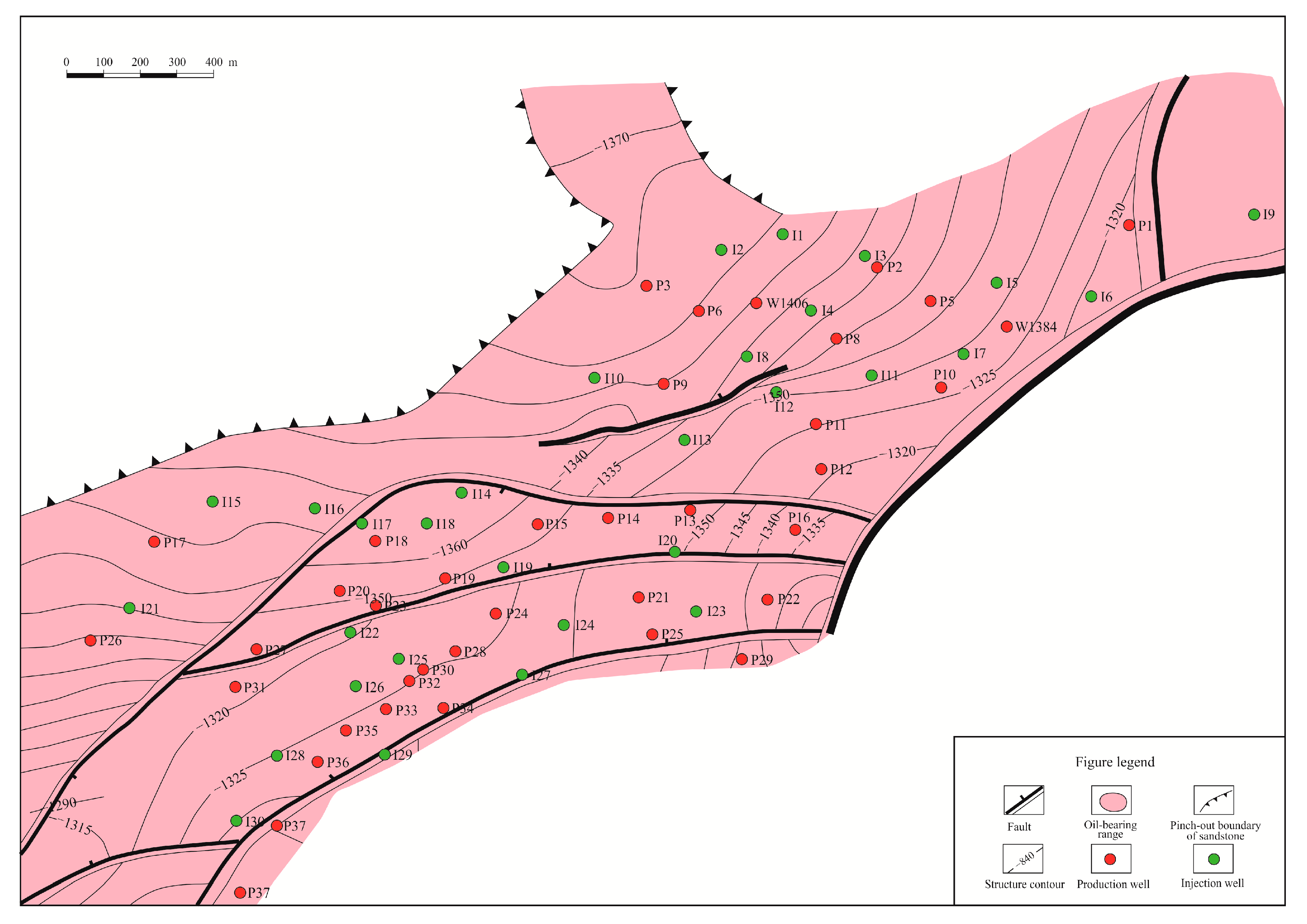
3.1. Overview of the Block

GX Block of an eastern China oilfield is in the north wing of the Gangxi draped anticline. It is a serpentine fluvial deposit on a floodplain. Its main lithology is argillaceous siltstone, and its cement is mainly argillaceous. The oil-bearing strata are the Minghuazhen Formation and Guantao Formation of the Upper Tertiary and have depths ranging from 805.4 to 1395.0 m. The original formation pressure was 10.85 MPa, and the temperature of the oil formation was 53.6 °C. GX Block was formally put into development in 1970, with waterflooding beginning in 1972. There are now 168 production wells and 112 injection wells in service, with a cumulative production of 7.27 million tons of oil and a combined water cut of 84.32%; see Figure 4.

GX Block has poor geological conditions, a high shale content, loose cementation, and poor diagenesis. It has been developed through perforation completion, water injection, and mechanical oil production. Owing to frequent changes to the working system, the production of oil wells, and other reasons, the proportion of casing-damaged wells is increasing, and many wells have been shut down because of casing damage. GX block is thus an area with serious and representative casing damage. How to effectively identify and predict casing damage and take preventive measures in advance is an urgent technical problem to be solved for this oilfield.

3.2. Data Processing

This study collected well data within the block, including a casing damage overview and geological, engineering, and development data, which amounted to more than 1.68 million pieces of data. Combined with production, pressure, sand production, operational history, and other data of the oil and water wells, the data were refined to single-well basic data, single-well sub-layer data, casing data, perforation data, and production data for a total of 295 factors, as shown in

Table 4. Data collection information.

Data Categories	Granularity	Samples Records	Main Features
Basic data	Well	446	Wellname, block, completion date, current well type, etc.
Sub-layer data	Well layer	>60,000	Wellname, layer, sand layer depth, porosity, permeability, oil saturation, lithology, casing state, etc.
Casing data	Casing interval	>3000	Wellname, steel grade, ID, OD, wall thickness, cement depth, etc.
Perforation data	Perforation interval	>10,000	Wellname, perforation method, perforation depth, perforation density, perforation number, etc.
Production data	Well	Oil wells: >74,000	Wellname, daily oil rate, daily liquid rate, monthly oil rate, monthly liquid rate, cumulative oil production, cumulative liquid production, water cut, oil pressure, casing pressure, etc.
		Water well: >37,000	Wellname, daily water injection, monthly water injection, cumulative water injection, oil pressure, casing pressure, etc.
	Well layer	Oil well: >1,000,000	Wellname, layer, daily oil rate, daily liquid rate, monthly oil rate n, monthly liquid rate, cumulative oil production, cumulative liquid production, water cut, etc.
		Water well: >500,000	Wellname, layer, daily water injection, monthly water injection, cumulative water injection, etc.

. The data processing is described as follows.

The original data were first preprocessed, which involved data quality control (Figure 5) and category coding of text-type data (

Table 5. Preprocessing of steel grade data.

No.	Steel Grades	Category Code	Normalized Values
1	J55	1	0
2	N80	2	0.25
3	P110	3	0.5
4	K55	4	0.75
5	D40	5	1

). The data characteristics were then expanded (in terms of the production pressure difference, liquid production intensity, maximum water injection volume, average water injection volume, standard deviation of the water injection volume, and the ratio of the casing outer diameter to the wall thickness without business meaning) to ensure the quality of the original data. Following analysis and processing, the features in the sample data included original features (i.e., original data) and extended features (i.e., extended data).

After the basic preprocessing of the obtained original data, feature integration and modeling feature design were carried out for the two granularities of the well and well layer. The data with well-layer granularity integrated the above original data according to the well name and layer or depth range fields. In addition to the original features, extended features such as the production differential pressure, outer casing diameter, and thickness ratio were added. The data with well-granularity integrated the above original data according to the well name. In addition to the original features, extended features such as the effective thickness of the single-well sub-layer and perforated interval data were introduced.

3.3. Analysis of Main Control Factors

After the block data were processed, the main controlling factors of casing damage were studied. It has been shown that casing damage is affected by many factors, including sand production, the reservoir temperature, the casing material, the cementing quality, the perforation method, and corrosion. The above influencing factors can be divided into geological factors, engineering factors, and development factors, with the geological factors being internal factors, and the engineering and development factors being external factors. The factors are summarized in Figure 6.

This study considered 295 factors in four areas (geology, engineering, development, and production) and adopted box plots, F-tests, and mutual information to qualitatively and quantitatively determine the main factors affecting casing damage and the weights of the factors from univariate and multivariate perspectives.

(1)

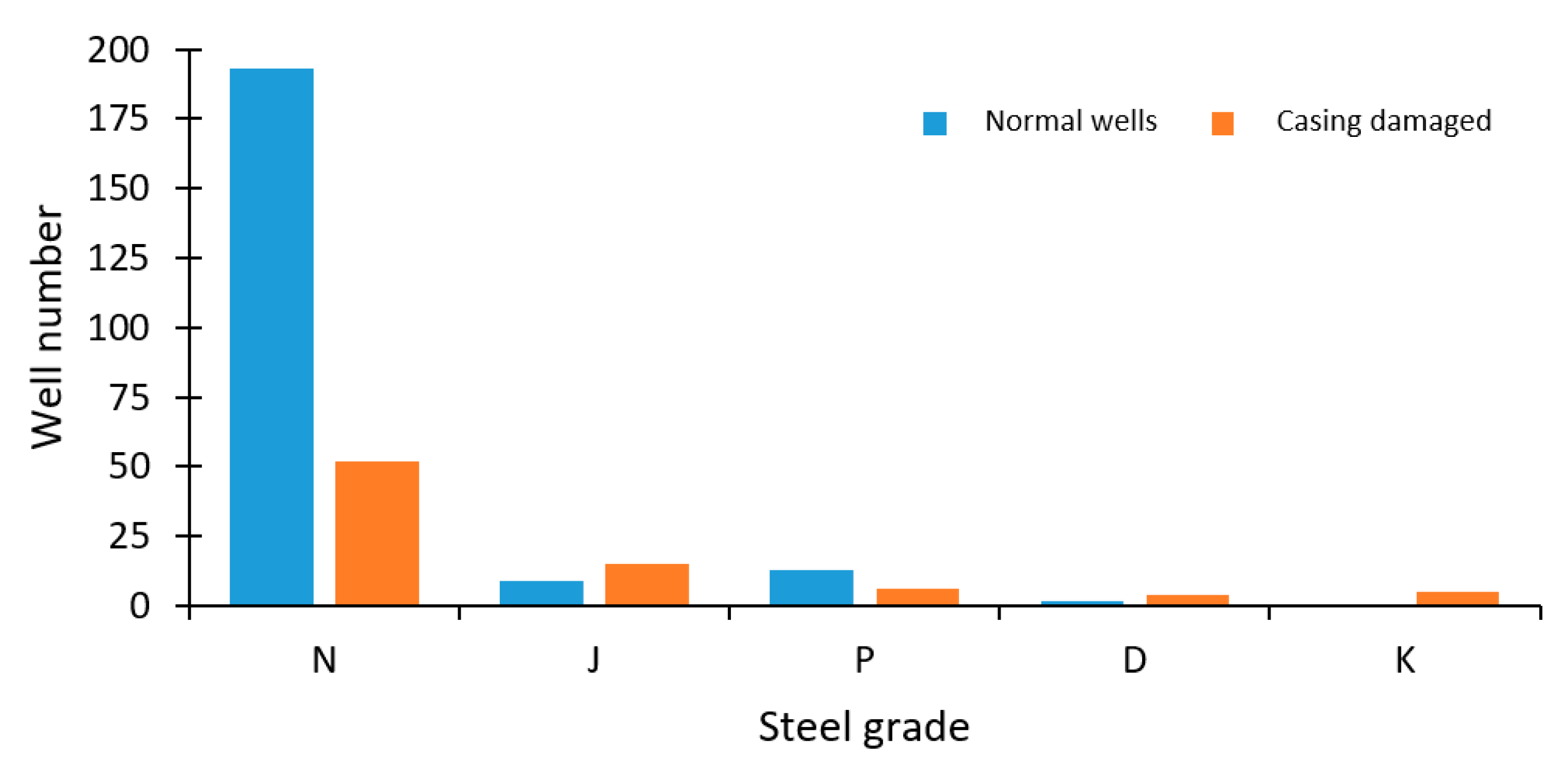
Univariate analysis based on box plots and bar charts

First, box plots were used to qualitatively analyze all influencing factors, as shown in Figure 7, where label 0 represents normal wells and label 1 represents casing-damaged wells.

Figure 7 shows that from the perspective of geological parameters, the sand layer thickness and permeability are higher for casing-damaged wells. From the perspective of production parameters, the oil production intensity, casing pressure, flow pressure, and calculated producing pressure drop are higher for casing-damaged wells, and from the perspective of engineering parameters, the perforation thickness and perforation number are higher for casing-damaged wells.

A bar chart was drawn to analyze the influencing factors of casing damage. Taking the steel grade at the level of well granularity as an example (Figure 8), the casing with steel grades N and P tends to suffer less casing damage.

(2)

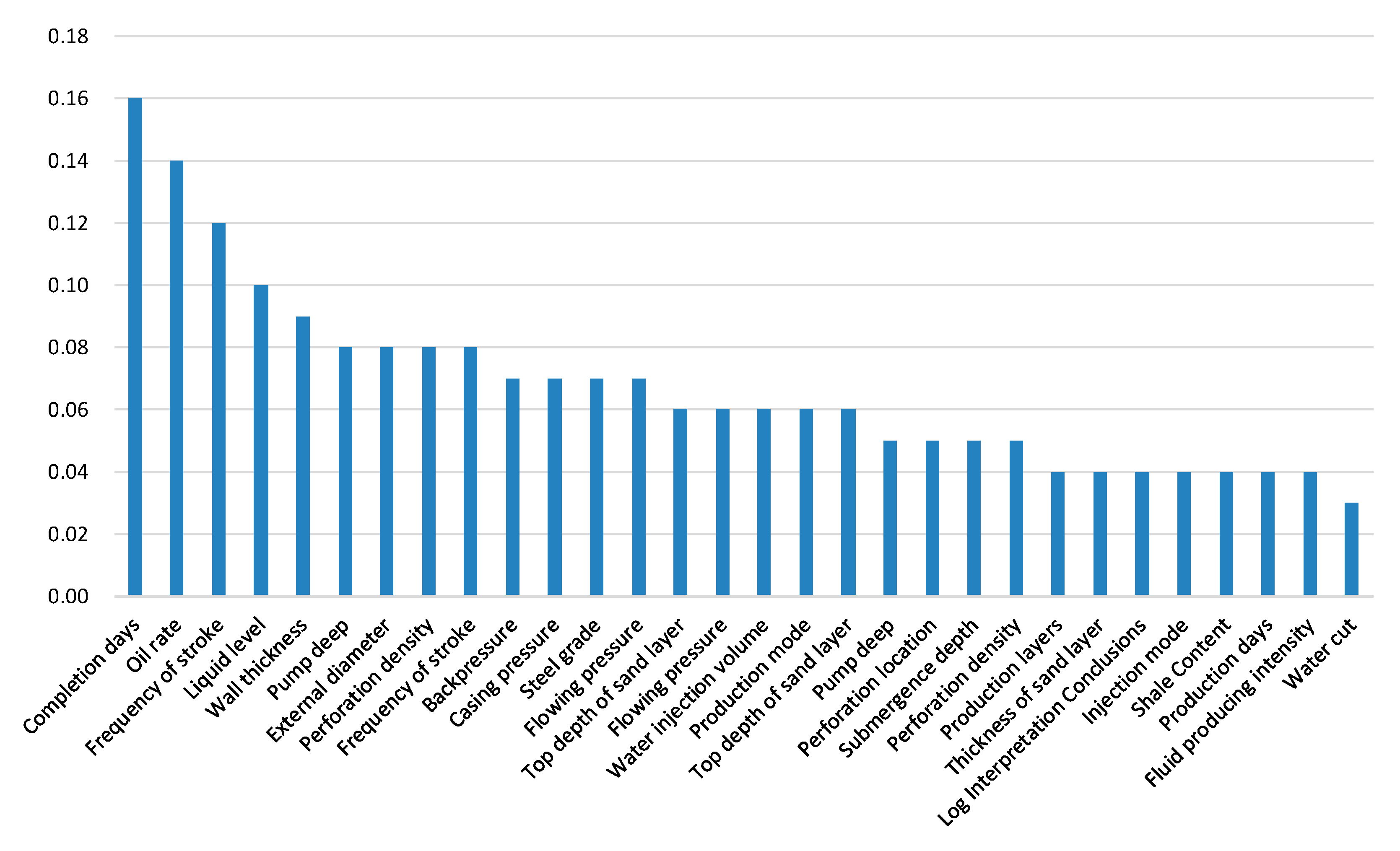
Multivariate quantitative study adopting the F-test and mutual information

In this study, the F-test and mutual information were adopted to obtain the influence weight of each factor at well and well-layer granularity.

Table 6. Results of the F-test (left) and mutual information (right) of data at well granularity.

Factors	F_Value	p_Value	Factors	Mi
Oil rate	57.61	0.00	Completion days	0.16
Frequency of stroke	33.51	0.00	Oil rate	0.14
Steel grade	22.09	0.00	Frequency of stroke	0.12
Submergence depth	20.98	0.00	Liquid level	0.10
Liquid level	18.23	0.00	Wall thickness	0.09
Production layers	18.09	0.00	Pump depth	0.08
Wall thickness	16.78	0.00	External diameter	0.08
Perforation location	16.17	0.00	Perforation density	0.08
Log Interpretation Conclusions	15.21	0.00	Frequency of stroke	0.08
Backpressure	14.56	0.00	Backpressure	0.07
Perforation thickness	11.73	0.00	Casing pressure	0.07
Water injection volume	10.79	0.00	Steel grade	0.07
Pump deep	10.53	0.00	Flowing pressure	0.07
Displacement	10.22	0.00	Top depth of sand layer	0.06
Water cut	8.24	0.00	Flowing pressure	0.06
Production layer	7.84	0.01	Water injection volume	0.06
Pump diameter	7.53	0.01	Production mode	0.06
Completion days	7.50	0.01	Top depth of sand layer	0.06
Fluid producing intensity	7.05	0.01	Pump deep	0.05
Casing pressure	6.63	0.01	Perforation location	0.05
Injection mode	6.02	0.01	Submergence depth	0.05
Top height of cement ring	5.59	0.02	Perforation density	0.05
Perforation density	5.27	0.02	Production layers	0.04
Top depth of sand layer	4.80	0.03	Thickness of the sand layer	0.04
Thickness of the sand layer	4.34	0.04	Log interpretation conclusions	0.04
Production days	4.14	0.04	Injection mode	0.04
Shale Content	3.86	0.05	Shale Content	0.04
Flowing pressure	3.60	0.06	Production days	0.04
Producing pressure difference	3.54	0.06	Fluid producing intensity	0.04
Oil pressure	3.16	0.08	Water cut	0.03

presents the calculation results of the two methods at well granularity.

The results of the F-test in Table 6 show that the oil production rate, frequency of stroke, and steel grade have a greater effect on casing damage. The results of the mutual information calculation show that the completion days, oil rate, and frequency of stroke have a larger effect on the casing damage.

A comparison of the two methods shows that the results of the mutual information calculation are similar to those of the F-test. However, a major advantage of using mutual information is that it can detect the relationship between multiple variables, whereas the F-test only expresses linear correlation. Combining the calculation results of the two approaches and the advantages of mutual information, the modeling of well granularity adopts the first 30 features of the mutual information calculation results in descending order (Figure 9).

3.4. Establishment of the Prediction Model

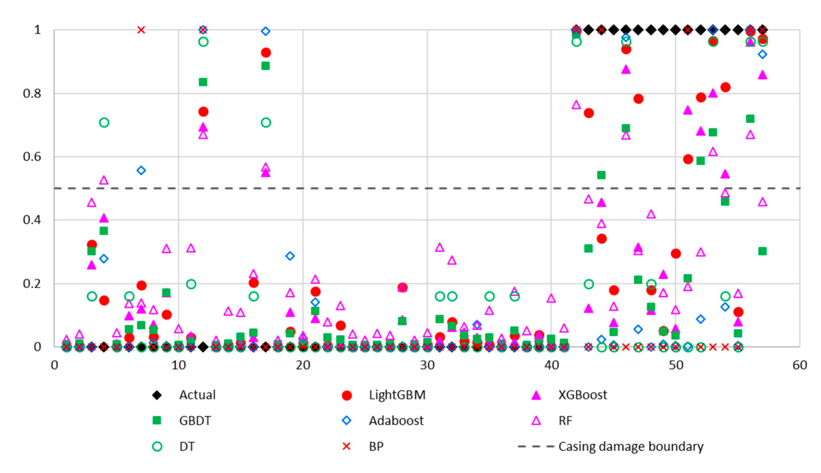
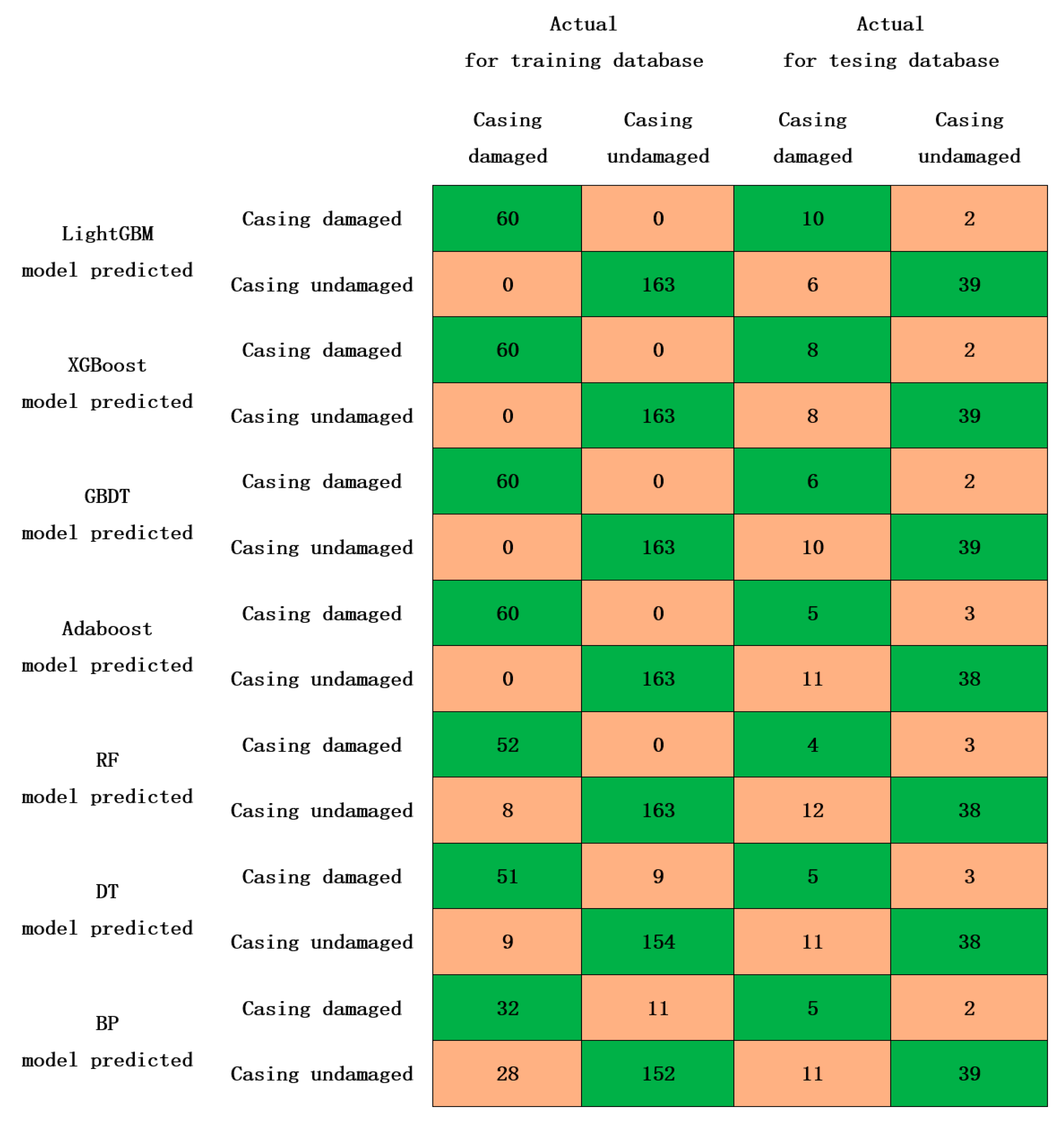
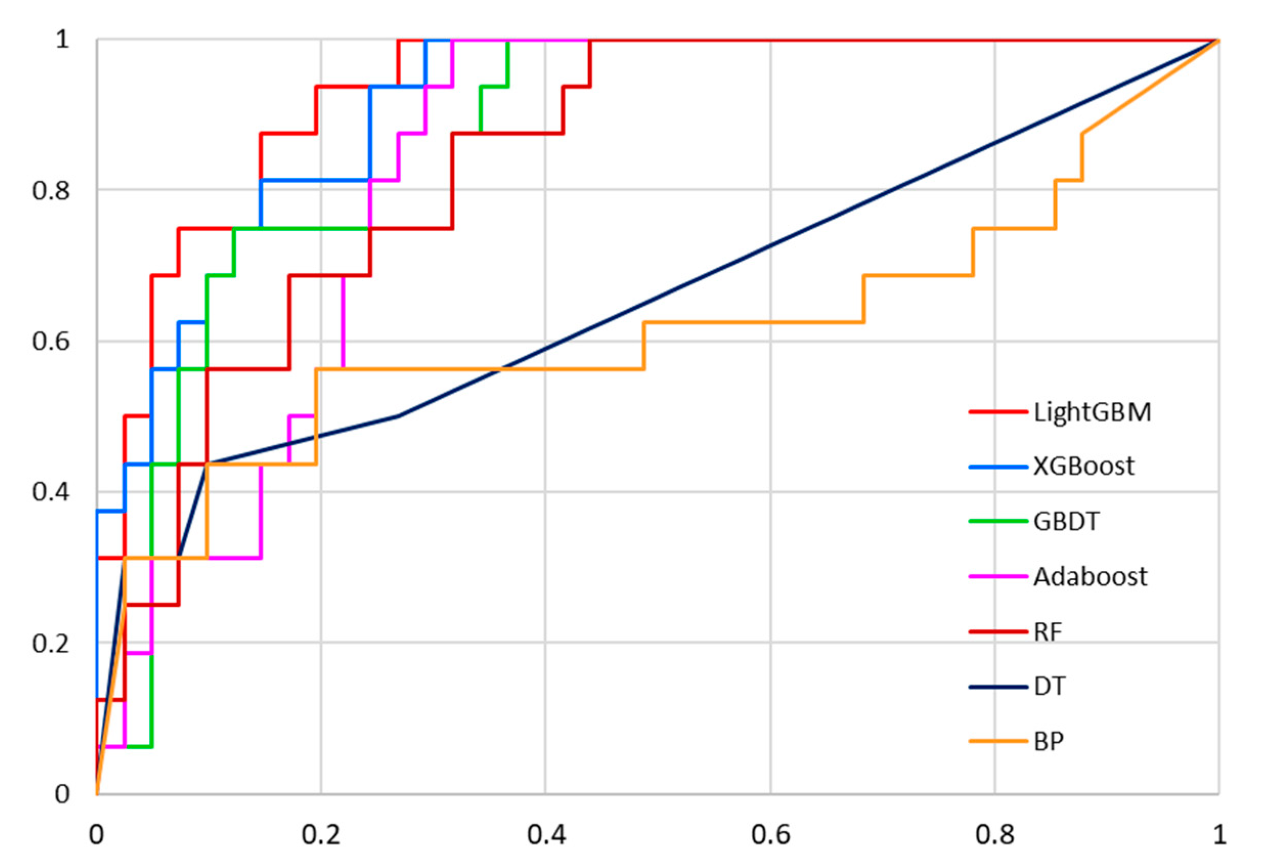
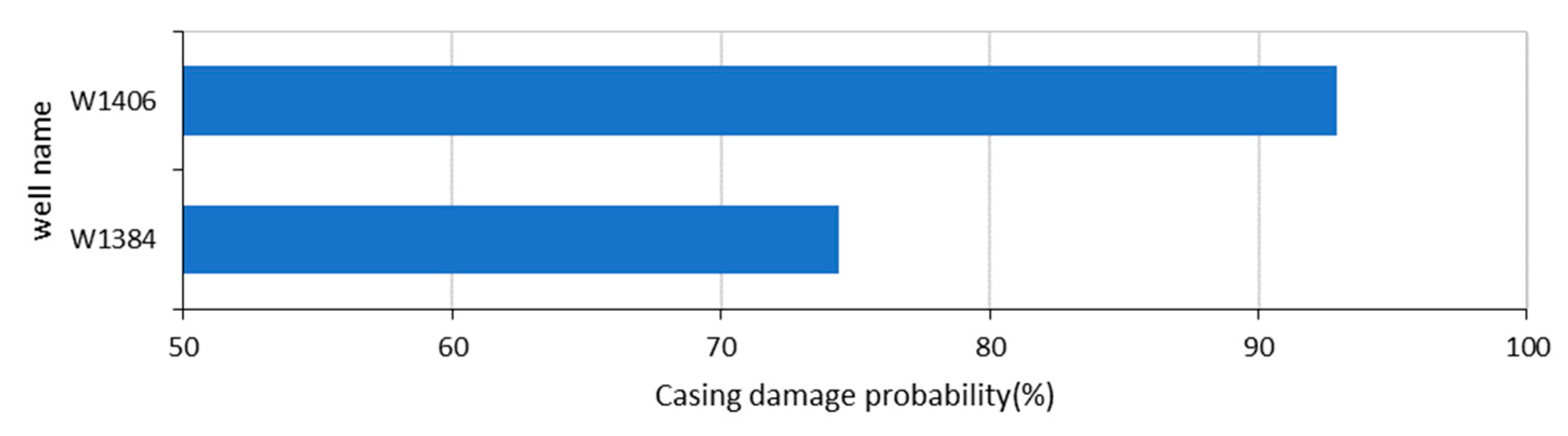
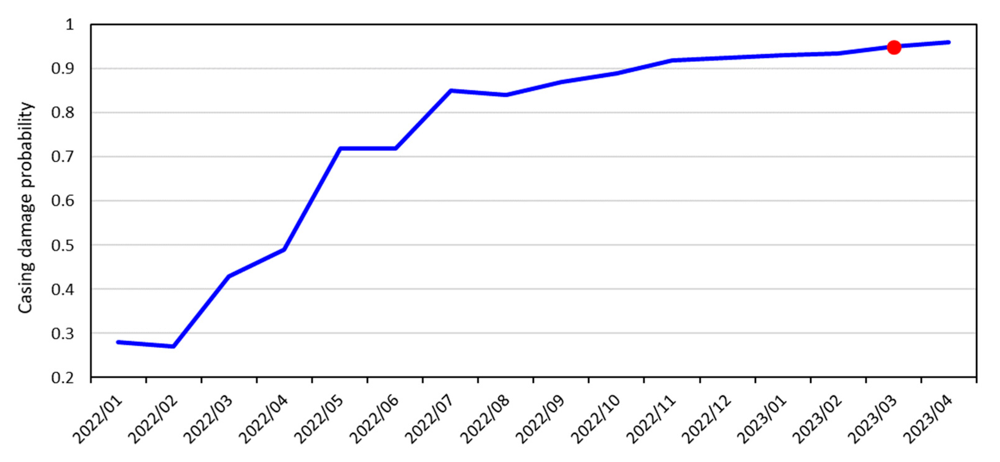
Following the determination of the influencing factors of casing damage to be input to the prediction model, the model was established for the two granularity schemes using the seven machine learning algorithms mentioned above. The parameters of the machine learning algorithms are given in

Table 7. Parameters of the machine learning algorithms.

Algorithm	Decision Tree (DT)	Random Forest (RF)	AdaBoost	GBDT	XGBoost	LightGBM	Neural Network (BP)
Major parameters	Max_depth	max_depth	max_depth	max_depth	max_dept	max_dept	hidden_layer_
	Max features	n_estimators	n_estimators	n_estimators	n_estimators	n_estimators	sizes, activation
		max_samples	max_features	subsample	subsample	subsample
		max_features		max_features	colsample_bytree	colsample_bytree

. A grid search was adopted to obtain the best choice of parameters. Taking the decision tree as an example, the minimum and maximum values of max_depth and max_features were first set, a series of parameter values were selected for each of the two hyperparameters and combined to obtain a list of candidate combination parameters, the candidates were input into the model, the score was calculated, and the parameters having the highest score were selected as the optimal choice for the model.

Five-fold cross-validation was then conducted to improve the robustness of the model, i.e., the data set was randomly divided into five portions, and four portions were taken for training the model and one portion for validating the model in each of the five validation cycles.

3.5. Results

Following parameter optimization and model verification, the failure probability was output by each model with the best parameter set. The prediction results for well granularity are shown in Figure 10.

As noted above, the probability prediction results are a binary classification. If the value is greater than 0.5, the output is 1, indicating possible casing damage, and if the value is less than or equal to 0.5, the output is 0, indicating no failure. Figure 11 quantitatively depicts the classification output of the different models as a confusion matrix. Figure 10 and Figure 11 show that the results of the different algorithms vary appreciably, but there is a common trend that the accuracy of identifying undamaged wells is higher than the accuracy of identifying damaged wells. It is assumed that this result is mainly due to the relatively small number of sample data for wells having casing failure.

The five evaluation indices are presented in

Table 8. Evaluation results of the well-granularity algorithm (mean ± standard deviation).

Algorithm	Accuracy (%)	Precision (%)	Recall (%)	F1 (%)	AUC (%)
LightGBM	87.50 ± 3.15	75.29 ± 8.80	78.33 ± 9.50	76.38 ± 6.17	91.73 ± 3.27
XGBoost	87.49 ± 4.20	81.91 ± 13.13	70.0 ± 18.26	73.69 ± 8.86	88.11 ± 3.99
GBDT	84.48 ± 3.90	74.54 ± 13.24	66.67 ± 11.79	68.97 ± 5.38	89.89 ± 2.04
Adaboost	87.07 ± 2.67	84.19 ± 10.94	65.00 ± 20.75	71.02 ± 8.66	87.69 ± 5.59
RF	87.06 ± 4.10	80.86 ± 14.84	71.67 ± 19.18	73.46 ± 8.33	90.45 ± 2.72
DT	84.91 ± 4.02	70.80 ± 8.08	71.67 ± 12.64	70.77 ± 9.11	81.84 ± 5.92
BP	67.66 ± 5.62	37.97 ± 8.58	41.67 ± 16.67	39.09 ± 12.03	58.24 ± 9.06

The AUCs of the models are shown in Figure 9.

, and the AUCs are plotted in Figure 12 for the quantitative comparison of the performance of the models.

Table 8 and Figure 12 present the accuracy of the seven algorithms for the case in this paper. Taking accuracy as the main evaluation index and comprehensively considering the balance of precision and recall (F1 value), a comparison of the results of the different models shows that LightGBM performs best, followed by XGBoost and the RF algorithm. This result is consistent with our perception of these common algorithms. The first two boosting algorithms are both advanced versions of the GBDT. LightGBM supports distribution calculation and can quickly process massive data, and it has a much less restrictive maximum depth, ensuring high efficiency while preventing over-fitting. Although XGBoost has a strong generalization ability, it automatically learns the split direction of missing values and customizes the loss function, and its prediction is thus more accurate. The RF algorithm is a bagging algorithm that avoids the overfitting problem of single decision trees and handles input samples with high-dimensional features. It evaluates the importance of individual features on the classification problem and the interaction between different features and it obtains good results for default value problems. Additionally, although the backpropagation neural network has a strong information synthesis ability and can fit various complex models, because of its black-box nature, it usually requires a larger amount of data. It is thus difficult to achieve good verification results for the backpropagation neural network in this case because of insufficient data.

In this study, we chose LightGBM as the algorithm, having the best results to build the prediction model for the well-granularity scheme. The main parameters of the algorithm were max_depth of 3, n_estimators of 50, colsample_bytree of 0.8, one subsample, a classification threshold of 0.5, 243 modeling dimensions, and 291 samples (76 casing-damaged layer samples for the positive classification and 215 non-casing-damaged layer samples for negative classification).

As mentioned above, the overall technical basis of the well-layer granularity analysis is the same as that of the well-granularity analysis. Therefore, only the evaluation results at the well-layer granularity are shown, omitting the specific process. The five evaluation indicators of each model are summarized in

Table 9. Evaluation results of algorithms at well-layer granularity (mean ± standard deviation).

Algorithm	Accuracy (%)	Precision (%)	Recall (%)	F1 (%)	AUC (%)
LightGBM	89.84 ± 10.29	69.72 ± 31.12	67.50 ± 14.25	66.85 ± 23.29	84.11 ± 13.61
XGBoost	90.14 ± 6.92	69.21 ± 29.89	60.0 ± 16.3	62.15 ± 19.72	82.21 ± 10.76
GBDT	87.05 ± 9.51	57.56 ± 32.92	62.5 ± 19.76	57.86 ± 24.59	82.35 ± 17.53
Adaboost	91.37 ± 5.27	72.48 ± 26.17	55.0 ± 16.77	61.96 ± 20.0	8 7.69 ± 5.59
RF	87.68 ± 8.69	64.0 ± 35.78	42.5 ± 18.96	48.65 ± 23.68	77.6 ± 10.05
DT	89.21 ± 4.47	82.0 ± 30.33	32.5 ± 14.25	42.33 ± 15.88	65.63 ± 13.87
BP	90.44 ± 4.12	81.71 ± 30.94	37.5 ± 8.84	50.37 ± 13.59	76.41 ± 5.14

.

Similar to the case for well granularity, the best algorithm for well-layer granularity was determined to be LightGBM, using the accuracy and the F1 value as the primary basis of evaluation.

The main parameters of the algorithm were max_depth of 3, n_estimators of 50, colsample_bytree of 0.8, one subsample, a classification threshold of 0.5, 31 modeling dimensions, and 406 samples (355 casing-damaged layer samples for positive classification and 51 non-casing-damaged layer samples for negative classification).

The optimal algorithm for the two granularity schemes was LightGBM.

Table 10. Comparison of the predictions of LightGBM modeling at different granularities.

Granularity	Accuracy (%)	Precision (%)	Recall (%)	F1 (%)	AUC (%)
Well	87.29 ± 3.77	80.69 ± 9.40	71.31 ± 11.38	74.99 ± 8.06	91.86 ± 3.77
Well-layer	92.45 ± 2.36	79.79 ± 13.43	60.81 ± 14.20	67.79 ± 11.27	93.95 ± 3.25

presents the results for the two granularity schemes. Both schemes had an accuracy of approximately 90% and a precision of approximately 80%. On the test data set, the prediction under the well-granularity scheme was better than that under the well-layer-granularity scheme.

The comparison of the results for the two granularity schemes in Table 10 shows that the well-granularity scheme outperformed the well-layer-granularity scheme. This result is consistent with the applicability of the two schemes, considering the small volume of data, coarse granularity, and incomplete data of the single-well sub-layer of casing-damaged wells. The well-granularity scheme was thus preferred in establishing a model for this case as it provides a more balanced prediction. The continuous accumulation of data on the geological and engineering parameters of layered granularity and the continuous improvement of production data further support the use of the well-granularity modeling scheme.

Using the finally determined well-granularity LightGBM algorithm for modeling, the casing damage probability was predicted for 280 wells in Oilfield A, the casing damage probability of each well was calculated for different periods, and the curve of casing damage probability changing with time was drawn for each well. The timing of casing damage can be predicted from the trend of the curve. According to this forecast, the two wells facing the greatest risk of casing damage are presented in Figure 13.

Applying the model at regular time intervals to predict the risk of casing damage, such as in the example of well W1406 (Figure 14), it was found that the curve of the casing damage probability had an obvious upward trend. The prediction curve for well W1406 indicates that damage to the casing may have already occurred in April 2022 (with the probability reaching 0.5), and the casing damage risk will be extreme in March 2023 (the red dot, with the probability approaching 1).

In confirming the predictions with oilfield observations, it was found that six of the ten wells having the highest casing-damage risk had indeed been damaged. This damage had not previously been noted by technicians. The prediction results are thus consistent with the actual situation and provide a reference for the prevention and treatment of casing damage.

4. Research Limitations

The present study had the following limitations.

(1)

The identification of damaged wells faced the common modeling problem of insufficient failure data to find a correct solution.

(2)

Although two schemes based on well and well-layer granularities were proposed and well-layer granularity was adopted to build the model, there were incomplete sub-layer data to support our recommendations.

(3)

There remain instabilities in the prediction model. The precision, recall, and F1 standard deviations of the validation set and the test set were large because different data divisions led to different training data distributions learned by the model, and the prediction law learned by the model was thus unstable. This situation can be improved by expanding the volume of data, especially for casing-failure wells.

5. Conclusions

The main contributions and conclusions of the study are as follows.

(4)

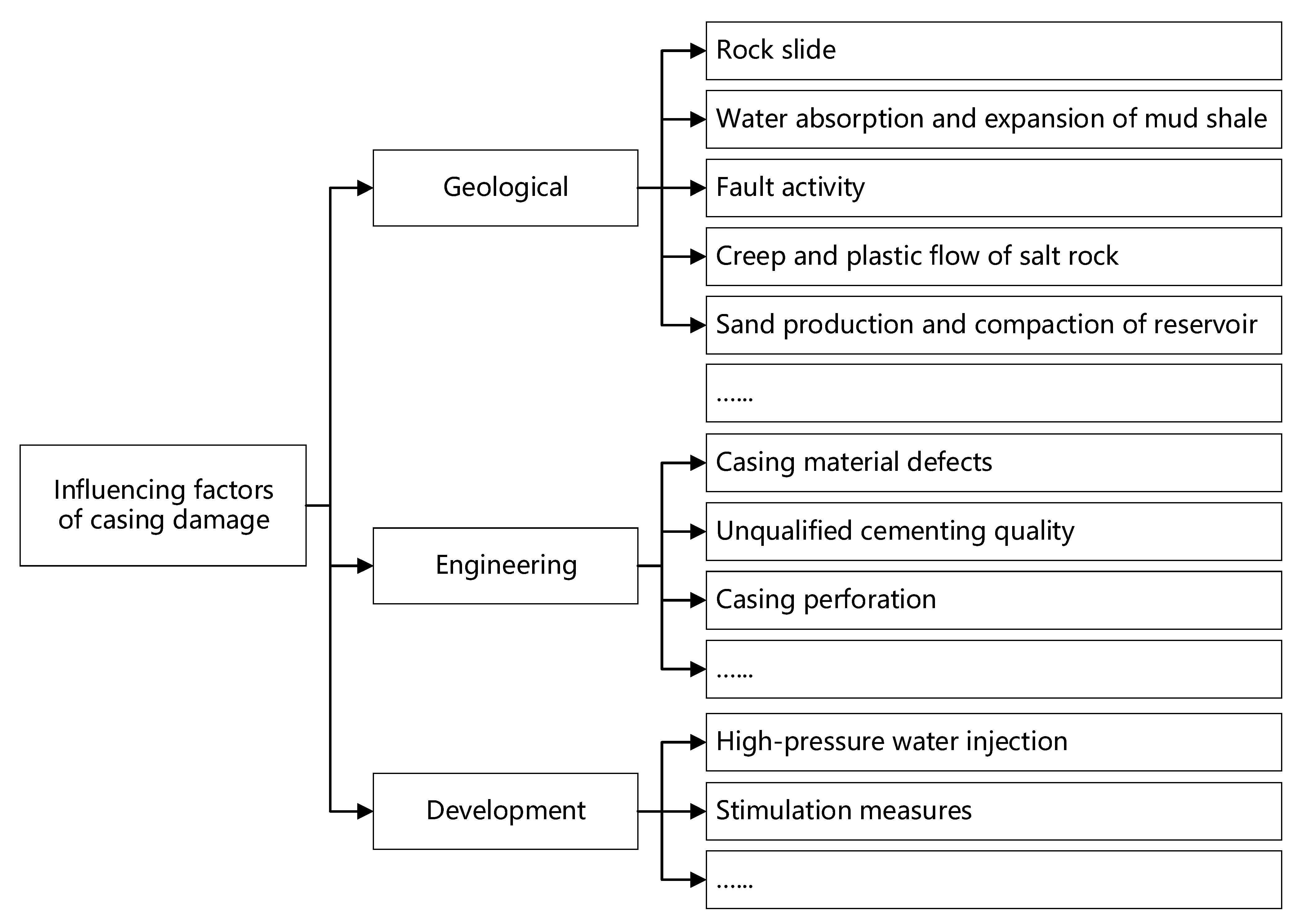
The study considered 295 factors in four areas (geology, engineering, development, and production) and adopted the F-test and mutual information to demonstrate and determine the main control factors, such as the completion days, oil rate, and wall thickness.

(5)

The study investigated and established a casing damage prediction model based on the LightGBM algorithm using the top 30 controlling factors as the input data, following a comprehensive comparison of seven algorithms, namely the decision tree, RF, AdaBoost, GBDT, XGBoost, LightGBM, and backpropagation neural network algorithms, in terms of five evaluation indices.

(6)

The study used different modeling schemes at well and well-layer granularity. The prediction accuracy was higher for the well granularity scheme, with a precision exceeding 80% and recall exceeding 70%.

(7)

Oilfield data showed that the results of the prediction model are in good agreement with actual casing damage. The prediction model can effectively guide the daily production of an oilfield, extend the life cycles of oil and water well casings, and improve the efficiency of oilfield development.

References

1. Noshi, C.I.; Amani, M. Casing string fatigue: No more. In Proceedings of the Presented at Offshore Technology Conference, Houston, TX, USA, 2 May 2022. [Google Scholar] [CrossRef]
2. Li, M. Study on Creep Casing Failure Mechanism of Mudstone in Shallow Formation. Master’s Thesis, Northeast Petroleum University, Daqing, China, 2021. [Google Scholar]
3. Zhang, X.; Wang, L.; Meng, F. Bayesian neural network approach to casing damage forecasting. Prog. Geophys. 2018, 33, 1319–1324. Available online: https://kns.cnki.net/kcms/detail/11.2982.P.20180122.1050.050.html (accessed on 9 March 2018).
4. Fang, J.; Yue, B.; Zhao, H. Analysis of surface loading on casing and cement sheath under nonuniform geologic stress. J. China Univ. Pet. 1997, 21, 46–48. [Google Scholar]
5. Fang, J.; Gu, Y.; Mi, F. A numerical analysis of casing collapse under nonuniform load. China Pet. Mach. 1999, 27, 34–37. [Google Scholar]
6. Zhang, G.; Liu, C. Effect of creep of surrounding rocks on deformation of oil well casing. Chin. J. Rock Mech. Eng. 2000, 19, 971–975. [Google Scholar]
7. Diao, S.; Yang, C.; Liu, J. Mechanism of seepage induced casing damage and numerical simulation. Rock Soil Mech. 2008, 29, 327–332. [Google Scholar] [CrossRef]
8. Jiang, X.; Zhang, S.; Wang, Z. Evaluating method of the geological-factor risks of the casing damage based on the certainly factors. Pet. Geol. Oilfield Dev. Daqing 2016, 35, 104–108. [Google Scholar]
9. Fu, L.; Ma, L.; Wang, W. Cause and repair & maintenance measures of casing in oil and water well. Pet. Drill. Tech. 2002, 30, 53–56. [Google Scholar]
10. Xiao, Y. Research on Casing Damage Mechanism, Detection Method and Casing Damage Prediction. Master’s Thesis, Daqing Petroleum Institute, Daqing, China, 2007. [Google Scholar]
11. Wang, T.; Yang, S.; Zhu, W. Law and countermeasures for the casing damage of oil production wells and water injection wells in tarim oilfield. Pet. Explor. Dev. 2011, 38, 352–361. [Google Scholar] [CrossRef]
12. Fang, X. Casing damage analysis and preventing measures under complex conditions. Pet. Geol. Recovery Effic. 2013, 20, 94–98+101. [Google Scholar] [CrossRef]
13. Zhang, J. Study on Casing Damage Causes and Prediction Methods in Complex Faulted Basins. Doctoral Thesis, Ocean University of China, Qingdao, China, 2014. [Google Scholar]
14. Zheng, X. Discussion on damage and prevention of oil well casing under complex conditions. Chem. Eng. Equip. 2019, 76+90. [Google Scholar] [CrossRef]
15. Lian, Z.; Zhao, G.; Zhang, X. Analysis of computer simulation of three-dimension loads acting on casing. J. Southwest Pet. Univ. Sci. Technol. Ed. 1995, 17, 101–108. [Google Scholar]
16. Meng, F.; Zhang, J.; Yang, C.; Yu, W.; Chen, Y. Three-dimensional finite element numerical simulation and physical experiment for magnetism-stress detecting in oil casing. J. Ocean. Univ. China 2015, 14, 669–674. [Google Scholar] [CrossRef]
17. Deng, J.; Liu, S.; Shi, D. Calculation of elastoplastic deformation of wellbore in soft mudstone using lagrangian method. J. Geomech. 1999, 5, 35–39. [Google Scholar]
18. Han, L.; Yin, F.; Yang, S.; Liu, W.; Deng, Y. Coupled seepage-mechanical modeling to evaluate formation deformation and casing failure in waterflooding oilfields. J. Pet. Sci. Eng. 2019, 180, 124–129. [Google Scholar] [CrossRef]
19. Xie, R.; Liu, J.; Zhang, Y. Detecting casing damages with electromagnetic defect detection log and its applications. Well Logging Technol. 2003, 27, 242–245. [Google Scholar] [CrossRef]
20. Zhang, X.; Zhang, X.; Zhao, G. Prediction of casing damage through sequential fussy synthetic evaluation. J. Southwest Pet. Inst. 1996, 18, 77–80. [Google Scholar]
21. Zhao, P.; Li, C.; Lu, J. Modeling for a class of nonlinear system and its application in predicting the casing failure trend. Pet. Explor. Dev. 1997, 24, 86–89. [Google Scholar]
22. Cheng, L.S.; Luo, Y.; Ding, Z.P. Fuzzy comprehensive evaluation model for estimating casing damage in heavy oil reservoir. Pet. Sci. Technol. 2013, 31, 1092–1098. [Google Scholar] [CrossRef]
23. Wang, Q.; Zhang, L.; Hu, J. Real-time risk assessment of casing-failure incidents in a whole fracturing process. Process Saf. Environ. Prot. 2018, 120, 206–214. [Google Scholar] [CrossRef]
24. Zhou, Y.; Jia, J. Research on new method for predicting of casing damage. Drill. Eng. 2009, 36, 230–234. [Google Scholar]
25. Zhou, Y.; Jia, J.; Li, R. Dynamic prediction method of casing damage based on rough set theory and support vector machine. J. China Univ. Pet. 2010, 34, 71–75. [Google Scholar]
26. Yan, X.; Xu, Z.; Yang, X. Life prediction analysis of gas well casing string under complex conditions based on support vector machine. In Proceedings of the 8th National MTS Material Testing Academic Conference, Tainan, China, 24–25 September 2010; pp. 560–564. [Google Scholar]
27. Zhao, Y.; Jiang, H.; Li, H. Research on predictions of casing damage based on machine learning. J. China Univ. Pet. 2020, 44, 57–67. [Google Scholar]
28. Zhu, J.; Wang, S.; Liu, H.; Wang, J. Multi-factor evaluation technology for casing damaged wells. In Proceedings of the International Oil & Gas Conference and Exhibition in China, Beijing, China, 5 December 2006. [Google Scholar]
29. Huang, J.; Meng, F.; Zhang, X.; Yang, G. Application of genetic neural network based on pca in prediction of casing damage. J. Xi’an Shiyou Univ. Nat. Sci. Ed. 2018, 33, 84–89. [Google Scholar]
30. Wang, L.; Meng, F.; Zhang, X. Application of bayesian neural network based on hmc algorithm in casing damage forecast. Inn. Mong. Petrochem. Ind. 2020, 46, 9–12. [Google Scholar]
31. Noshi, C.I.; Noynaert, S.F.; Schubert, J.J. Failure predictive analytics using data mining: How to predict unforeseen casing failures? In Proceedings of the Abu Dhabi International Petroleum Exhibition & Conference, Abu Dhabi, United Arab Emirates, 12 November 2018. [Google Scholar]
32. Noshi, C.; Noynaert, S.; Schubert, J. Data mining approaches for casing failure prediction and prevention. In Proceedings of the International Petroleum Technology Conference, Beijing, China, 22 March 2019. [Google Scholar]
33. Song, M.; Zhou, X. A casing damage prediction method based on principal component analysis and gradient boosting decision tree algorithm. In Proceedings of the SPE Middle East Oil and Gas Show and Conference, Manama, Bahrain, 15 March 2019. [Google Scholar]
34. Tang, Q.; Wu, H.; Teng, G.; Bu, H.; Tan, C.; Liu, J.; Zhang, X.; Zhang, Y.; Yan, W.; Deng, J. Prediction of casing damage in unconsolidated sandstone reservoirs using machine learning algorithms. In Proceedings of the 2019 IEEE International Conference on Computation, Communication and Engineering, Fujian, China, 8–10 November 2019. [Google Scholar]
35. Tan, C.; Wu, H.; Liu, J.; Yan, W.; Deng, J.; Zhang, Y.; Tang, Q.; Bu, H. A novel data mining approach in preventing casing damage of oil production wells. In Proceedings of the 2019 IEEE Eurasia Conference on IOT, Communication and Engineering, Yunlin, Taiwan, 3–6 October 2019. [Google Scholar]
36. Carpenter, C. Data mining effective for casing-failure prediction and prevention. J. Pet. Technol. 2019, 71, 55–56. [Google Scholar] [CrossRef]
37. Xue, J. Casing damage classification method using random forest algorithms. J. Phys. Conf. Ser. 2020, 1437, 012131. [Google Scholar] [CrossRef]
38. Li, T. Research on the method of applying machine learning to predict casing damage. Master’s Thesis, China University of Petroleum, Beijing, China, 2020. [Google Scholar]
39. Noshi, C.I.; Amani, M. Data driven physics-guided casing fatigue life estimation. In Proceedings of the Offshore Technology Conference, Houston, TX, USA, 4 May 2022. [Google Scholar] [CrossRef]
Figure 1. Workflow of the intelligent casing damage prediction method.
Sustainability 14 14733 g001
Figure 2. Example of a box plot.
Sustainability 14 14733 g002
Figure 3. Predicted and forecast probability of casing damage for a well.
Sustainability 14 14733 g003
Figure 4. Well pattern map of GX Block (bottom of the Ming3 oil formation).
Sustainability 14 14733 g004
Figure 5. Preprocessing of wall thickness data.
Sustainability 14 14733 g005
Figure 6. Influencing factors of casing damage.
Sustainability 14 14733 g006
Figure 7. Box plots of the characteristics at well-layer granularity.
Sustainability 14 14733 g007
Figure 8. Bar chart of the well numbers of different steel grades at well granularity.
Sustainability 14 14733 g008
Figure 9. Main (top 30) control factors at well granularity.
Sustainability 14 14733 g009
Figure 10. Casing damage probability predictions of the different models.
Sustainability 14 14733 g010
Figure 11. Confusion matrix of the casing damage prediction.
Sustainability 14 14733 g011
Figure 12. Comparison of the AUCs of the well-granularity prediction models.
Sustainability 14 14733 g012
Figure 13. The two wells having the highest probability of casing damage among normal wells in Oilfield A.
Sustainability 14 14733 g013
Figure 14. Curve of the casing damage probability versus time for well W1406.
Sustainability 14 14733 g014