Abstract
In harsh offshore environmental conditions, the monopile foundations supporting offshore wind turbines must be designed for lateral loads such as winds, waves, and currents. The Beam on Nonlinear Winkler Foundation (BNWF) method has been widely used because of its clear concept and lower calculation cost. The selection of a reasonable p–y curve is critical to the calculation accuracy of this method. This paper clarified the defects of widely used API p–y curves for soft clays and then proposed a new p–y curve with better versatility and applicability. The suitability of the proposed p–y curve was validated by comparing it with the calculation results from the three-dimensional finite element method (3D FEM). Compared with the API p–y curve, the proposed p–y curve can better predict the lateral behavior of large-diameter piles in soft clays, such as the load–displacement curve of the pile head, lateral deflection profile, and bending moment profile. The research findings can provide guidance for the design of monopile foundations supporting offshore wind turbines in soft clays.
1. Introduction
Natural resources such as coal, petroleum, and natural gas are being consumed at an alarming rate, hence many countries are actively promoting green and sustainable new energy technologies. Wind energy is one of the most promising new energies due to its advantages of cleanness and renewability. In addition, compared with land-based wind energy, offshore wind energy is attractive for its various advantages including high speed, low wind shear, low turbulence, and high output. The urgent demand for wind power is promoting the development of construction technology for offshore wind turbines (OWTs) [1]. The design of the foundations supporting OWTs is extremely important because it may account for as much as 30% of the total cost of a typical offshore wind project [2,3]. Nonetheless, the large diameter monopile foundation remains by far the most popular foundation type being deployed in more than 75% of the currently installed OWTs [4,5]. In harsh offshore environmental conditions, pile foundations must be designed for lateral loads because OWTs are always subjected to such loads caused by winds, waves, and currents.
The Beam on Nonlinear Winkler Foundation (BNWF) method based on the p–y curve is widely used to analyze the behavior of laterally loaded piles. McClelland and Focht [6] first proposed the concept of a p–y curve by comparing the measured curve of lateral soil resistance versus the pile lateral deflection with the soil stress–strain curve in the consolidated undrained tests. Matlock [7] proposed a p–y curve model for piles installed in clay based on limited pile load tests at the Sabine River site, which was adopted by the API RP 2GEO (American Petroleum Institute (API)) [8] and is widely used in industry. In the BNWF approach, the pile is simulated as an elastic beam while the soil is idealized as a series of discrete nonlinear springs along the depth of the pile. The nonlinear p–y springs describe the relationship between the local lateral soil resistance p and the pile lateral relative displacement y. The BNWF method based on the p–y curve is actually a simplified method ignoring the soil continuity.
In recent decades, some new p–y curves for soft clay have been proposed to analyze the lateral behavior of piles. The hyperbolic equation, initially proposed by Kondner [9] and later identified by Georgiadis et al. [10] as a suitable formulation, is used to define the shape of the p–y curves. Dewaikar and Patil et al. [11] developed an improved method for the construction of hyperbolic p–y curves, in which the initial stiffness of the p–y curve is taken to be increasing with depth. Jeanjean [12] proposed a hyperbolic tangent p–y curve and verified its rationality using the centrifugal test and finite element simulation results of pile in clays. Klinkvort and Hededal [13] performed a series of centrifuge tests to investigate the behavior of a rigid pile loaded with a high eccentricity and presented a reformulation of the p–y curve. Rathod et al. [14] developed new p–y curves for piles located on crests of soft clay with different sloping ground surfaces under static lateral loading by carrying out a series of laboratory model tests. Zhu et al. [15] modified the hyperbolic tangent p–y curve by introducing an additional constant and verified its rationality using the field tests of offshore driven piles. Xu et al. [16] found that the hyperbolic method yields larger prediction errors than the API method and proposed a modified p–y approach based on field measurements. The p–y curve method has been developed to better simulate lateral responses based on model tests and numerical simulation results [17,18,19,20,21,22,23,24]. The above research mainly focus on the p–y curve under lateral monotonic loads.
The pile cyclic lateral response was also analyzed by developing cyclic p–y hysteresis curves based on the Beam on Nonlinear Winkler Foundation (BNWF) method. In these models, some pile–soil interaction characteristics are simulated using specific components such as spring, dashpot, drag cell, and gap cell to capture the dynamic hysteretic behavior of the soil–pile interface [25,26,27,28,29]. However, the introduction of too many components usually makes the implementation of the model more complex. In addition to the p–y method, the three-dimensional finite element method (3D FEM) was also used to analyze the lateral response of piles even though it requires larger costs of calculation [30,31,32,33,34,35,36,37,38]. The 3D FEM can better simulate the pile–soil interaction because both the pile and soil are simulated by continuum elements. Compared with the method, although discrete the p–y springs do not rigorously capture the soil continuum behavior, the BNWF method based on the p–y curve has still been widely utilized because of its clear concept and less calculation cost.
At present, the API p–y curve for soft clay [8], which is most widely used in industry, is proposed based on the specific field test of small diameter piles. Its applicability to larger diameter pile foundations, such as large-diameter steel pipe piles for offshore wind turbines, has been questioned. P–y curves with better applicability urgently needs to be developed. This research has two main objectives: (a) clarify the defects of widely used API p–y curve for soft clays and (b) develop a new p–y curve of soft clay with better applicability for large diameter monopile foundations.
In order to achieve the above research purposes, the BNWF method based on the p–y curve and three-dimensional finite element method for analyzing the lateral responses of monopile are developed based on ABAQUS software; then, the accuracy of the proposed two methods are verified using the field test results of pile in soft clays [7]. Subsequently, the lateral responses of monopiles with different diameters are simulated employing the two methods. The defects of the API p–y curve are clarified by comparing the calculated results obtained by the two methods. Based on the above findings, a new p–y model for soft clay is proposed and the good applicability of the model to large diameter monopiles is validated by the above three-dimensional numerical simulation results. The novelty of this study is that a new p–y model with variable parameters was proposed, which is more versatile and offers a wider applicability to represent different soft clay and pile diameters. Compared with the API p–y curve, the proposed p–y curve can better predict the lateral behavior of large diameter monopiles in soft clays.
2. Two Methods for Analyzing Lateral Responses of Piles in Soft Clays
2.1. Beam on Nonlinear Winkler Foundation (BNWF) Method
The BNWF model is developed based on ABAQUS software [39] to simulate the lateral monotonic load tests on teel pipe piles installed in soft clay at a site near the Sabine River [7]. The test pile had an outer diameter of 0.324 m with a wall thickness of 12.7 mm. The total length of the pile was 13.1 m with an embedded depth of 12.8 m. The lateral load was applied at 0.3 m above the ground surface. The average undrained shear strength of clays = 14.4 kPa, effective unit gravity = 7.85 kN/m3, elastic modulus of pile material EP = 210 GPa, density = 1820 kg/m3, and Poisson’s ratio = 0.33 were all utilized.
The schematic diagram of the BNWF model is shown in Figure 1. The pile is discretized by 128 two-dimensional beam column elements (B21 element) and the length of each element Le = 0.5 m. A nonlinear spring element is set at each element node to simulate the pile–soil interaction. The elastic modulus of the nonlinear spring is set according to the API p–y curve for soft clay. The spring resistance force F = p · Le · D (D is the outer diameter of the pile). The continuous variation of the elastic modulus of spring reflects the nonlinear relationship between the spring resistance force F (or lateral soil resistance) and the spring displacement y (the pile lateral relative displacement). The API p–y formula and relevant parameter values for this study are as follows:
where p is the mobilized lateral resistance (kPa); y is the local pile lateral displacement (m); is the pile lateral displacement at half of ultimate soil resistance (m); and , is the strain at one-half the maximum deviator stress in laboratory undrained compression tests of undisturbed soil samples. = 0.02 in this study. D is the pile diameter and D = 0.324 m. is effective unit weight of soil (kN/m3) and = 7.85 kN/m3. is the ultimate resistance (kPa); for and for . is the undrained shear strength (kPa) and = 14.4 kPa; z is the depth below the original seafloor (m); J is the dimensionless empirical constant with values ranging from 0.25 to 0.5 having been determined using field testing, and J = 0.5 in this study.
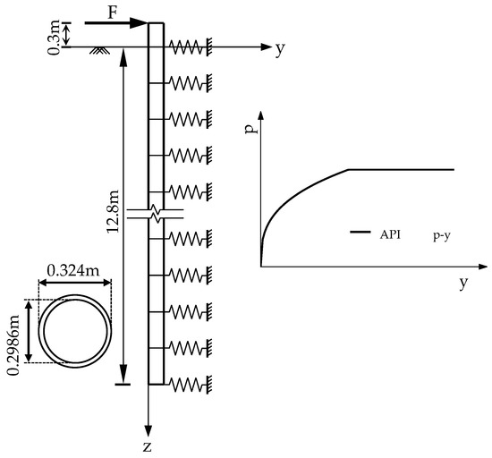
Figure 1.
Schematic diagram of BNWF model for laterally loaded pile in soft clays.
Figure 2a,b compare the calculated lateral deflection and bending moment profiles along the pile and those evaluated from the field measurements for four different pile head load levels. It can be seen that the calculated responses agree well with the test results for all load levels despite the slight deviations. One reason for the slight deviation is that the soil strength is idealized as uniform strength, but it is not uniform in the field test. Another reason is the limitation of the BNWF method itself, i.e., it ignores the continuity of soil, which will cause the error of calculation. This good agreement demonstrates that the developed BNWF model based on ABAQUS software can well predict the increase in lateral deflection and bending moment profiles with the increasing load level and the location of the maximum bending moment for different load levels. It also demonstrates the ability of the developed model to predict the lateral monotonic behavior of the pile in soft clays.
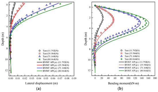
Figure 2.
Comparison between calculated and measured test results based on the BNWF method. (a) Lateral deflection profile (b) Bending moment profile.
2.2. Three-Dimensional Finite Element Method (3D FEM)
A three-dimensional finite element model is established by employing the finite element software ABAQUS to simulate the interaction between soft clay and the pile foundation considering the specific conditions for Matlock’s filed tests. Exploiting the symmetries of the geometry and loading conditions, the model simulates only one half of the system, as shown in Figure 3, to improve the computational efficiency. A sensitivity study indicates that a model of size 20 D × 50 D (the cross section is a semicircle and D is the pile diameter) is sufficient to avoid boundary effects on the simulation results. The pile and the soils are all simulated using 5466 8-node linear brick elements with reduced integrations (C3D8R). Normal horizontal constraints are applied to the vertical boundaries and fixed constraints are applied to the bottom boundary. The top boundary is fully free. Lateral loads are applied to the pile according to the loading condition in the above field tests.
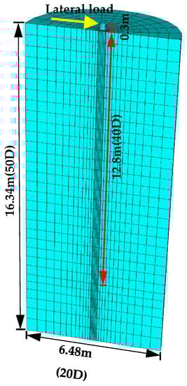
Figure 3.
Three-dimensional finite element model for laterally loaded pile in soft clays.
The interaction between the monopile and surrounding soil is simulated utilizing the surface-to-surface contact method. The surface of the pile is defined as the master surface (relatively stiff) and the soil surface in contact with the pile is defined as the slave surface (relatively soft). Hard contact is set in the normal direction of the contact surface, which allows separation between the interface elements when they are subjected to tension. The penalty contact method is used in the tangential direction. When the two surfaces are in contact, the interface behavior is governed by Coulomb’s friction theory. The critical friction shear stress at the contact surface can be expressed by in terms of the frictional coefficient and contact pressure , with = 0.3 in this study. When the shear stress at the contact surface exceeds , the tangential slip occurs.
The behavior of clay is simulated by employing the elastic-perfectly plastic constitutive model with Mises yield criterion. The model parameters include the soil elastic modulus, Poisson’s ratio, and shear strength, which can be determined using the laboratory tests or field tests. In this study, the model parameters are set according to the research of Matlock [7] and Hong et al. [37] as shown in Table 1. The material behavior of the hollow steel pipe pile is simulated using the linear elastic constitutive model. The model parameters are set according to the above steel properties. During the finite element simulation, geostatic stress balance analysis shall be carried out first, i.e., gravity is applied to the soil domain to establish the initial stress field. Meanwhile, the initial displacement field is set to 0. Then, lateral monotonic behavior of the pile is analyzed.

Table 1.
Constitutive model parameters and relevant calculation parameters.
Figure 4 shows the comparison between the calculated results and test results of the lateral deflection and bending moment profiles along the pile for four different pile head load levels. The calculated results agree with the test results in the overall trend although there is some deviation. One reason for the deviation is that the soil strength is idealized as uniform strength, but it is not uniform in the field test. Another reason is that it is a simplification to use the elastic-perfectly plastic constitutive model to simulate the stress–strain responses of the soil; when more advanced constitutive models are adopted, better calculation results can be expected. This comparison demonstrates that the developed three-dimensional finite element model based on ABAQUS software can well predict the lateral monotonic behavior of the pile in soft clays.
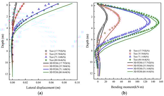
Figure 4.
Comparison between calculated and measured test results based on 3D FEM. (a) Lateral deflection profile (b) Bending moment profile.
3. Lateral Behavior Analysis of Monopiles with Different Diameters
3.1. Numerical Model
Two methods for analyzing horizontally loaded piles, namely the BNWF method and 3D finite element method, have been established and validated, respectively, in Section 2 above. It should be noted that the BNWF model is actually a two-dimensional simplified calculation model of the pile–soil interaction; the accuracy of the calculation results employing this model mainly depends on the rationality of the p–y curve, hence it has certain limitations when using the currently questionable API p–y curve. In comparison, the three-dimensional finite element method has a better applicability for different pile diameters and site soil characteristics, although the calculation cost is relative larger. In this chapter, the above two methods will be used to simulate the lateral behavior of monopiles with different diameters. Using 3D finite element simulation results as a relatively correct reference standard, the limitation of the current API p–y curve is clarified by comparing the calculation results obtained from two methods.
Four diameter piles (1 m, 2 m, 3 m, 5 m) were selected to build both two-dimensional BNWF models and 3D finite element models. The total length of all piles is 60 m with an embedded depth of 50 m and the wall thickness is 30 mm. A lateral load of 2 MN is applied at the pile head (10 m above the mud surface). The three-dimensional finite element models of the four diameter piles are shown in Figure 5. In the 3D numerical model, the constitutive models and material parameters of pile and soil, pile–soil contact condition, boundary conditions, etc. are consistent with those in Section 2 above, which will not be repeated here due to space limitations. The setting of the two-dimensional model is also consistent with those in Section 2 except for the different pile sizes.
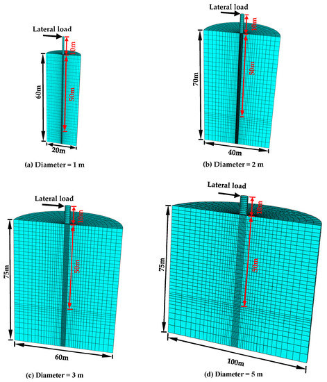
Figure 5.
3D finite element model for laterally loaded pile with different diameter in soft clays.
3.2. Comparison of Predicted Lateral Behavior for Two Methods
Figure 6 compares the lateral response of piles with various diameters obtained using the BNWF method based on the API p–y curve and 3D FEM when the pile head load equals 250 kN. It can be seen from Figure 6a that the nonlinearity of pile head load–displacement curve becomes more significant as the pile diameter decreases. The displacement of the pile head is greater for the smaller pile diameter under the same lateral load. The prediction result of displacement based on the BNWF method is larger than that of the 3D FEM, which indicates that the BNWF method underestimates the bearing capacity of piles. As shown in Figure 6b, the lateral deflection of the pile along the depth (range from −10 to 10) increases significantly as the pile diameter decreases, which is because the pile becomes more flexible due to the decrease in the stiffness. The lateral deflection profile obtained by the BNWF method is larger than 3D FEM and the difference between the two calculation results is more significant for the smaller diameter piles. It can be observed from Figure 6c that the bending moment of the pile along the depth increases significantly as the pile diameter increases and the location of the maximum bending moment moves downward gradually. The bending moment profile obtained by the BNWF method is larger than 3D FEM and the difference is more significant for the larger diameter piles. From the above comparison, it can be concluded that the BNWF method based on the API p–y curve will overestimate the deflection and bending moment and underestimate the ultimate bearing capacity of the large diameter pile.
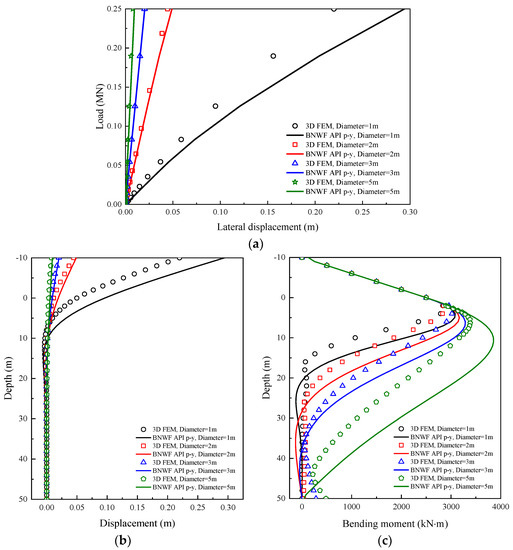
Figure 6.
Comparison of lateral response of piles obtained by BNWF method (API p–y curve) and 3D FEM. (a) Load–displacement curve of pile head. (b) Lateral deflection profile. (c) Bending moment profile.
3.3. Limitations of API p–y Curve for Soft Clay
The pile–soil interaction is simulated through the surface–surface contact mode for the 3D finite element model. The soil resistance value P at a certain depth of the pile shaft is calculated by extracting the contact force on the contact surface. Figure 7a shows the typical distribution of the calculated contact normal force (CNF) and the contact shear force (CSF) around the pile. Figure 7b shows the diagrammatic sketch for the x-direction component of the CNF (CNF1) and the x-direction component of the CSF (CSF1) at a certain position on the pile cross-section. Figure 7b,c shows the typical distribution of CNF1 and CSF1 around the pile. It can be observed that CNF1 is the largest in the x-axis direction and the smallest at the edges on both sides of the section (almost 0); on the contrary, CSF1 is the smallest (almost 0) in the x-axis direction and the largest at the edges on both sides of the section.
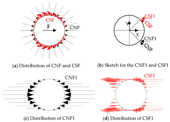
Figure 7.
Typical distribution of the calculated contact normal force (CNF) and contact shear force (CSF).
The soil resistance P at a certain depth of the pile shaft can be determined by the sum of CNF1 and CSF1 around the pile, as represented by:
where n is the number of nodes outside the pile cross-section at a certain depth of the pile shaft. Then, the p–y curve can be determined based on the numerical simulation results.
Figure 8 compares the API p–y curve with the p–y curve obtained using the 3D finite element method. These p–y curves correspond to different depths (depth = 1 m, 3 m, 5 m, and 10 m) for various pile diameters (diameter = 1 m, 2 m, 3 m, and 5 m). For these larger diameter piles, there are significant difference between the API p–y curve and the p–y curve obtained using the 3D finite element method. The comparison demonstrates: (1) the API p–y curve significantly underestimates the ultimate soil reaction of soft clays and the degree of the underestimation increases as the soil depth increases; (2) the API p–y curve significantly underestimates the initial stiffness of soft clays. This conclusion can well explain why the BNWF method based on the API p–y curve overestimates the deflection and bending moment while it underestimates the ultimate bearing capacity of the large diameter pile.
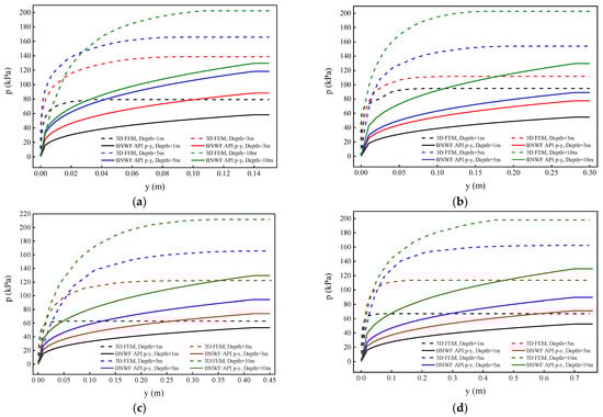
Figure 8.
Comparison of the API p–y curve and the p–y curve obtained by 3D finite element method. (a) Diameter = 1 m, (b) Diameter = 2 m, (c) Diameter = 3 m, and (d) Diameter = 5 m.
4. New p–y Curve for Soft Clay
4.1. New p–y Formula and Parameter Influence
In order to improve the shortcomings of the API p–y curve, a new p–y curve is proposed in this section, as shown in the formula:
where is the maximum shear modulus and is usually considered to be a multiple of for soft clay according to the engineering experience (e.g., typical range of = from 300 to 1800 ); parameters A and B control the shape of the p–y curve. is the ultimate lateral soil resistance, which is calculated based on the expression proposed by Murff and Hamilton [40] for shear strength profiles approximately linearly increasing with depth, i.e.,:
where is the undrained shear strength of soil at the point in question; is a nondimensional lateral bearing factor; is the soil submerged unit weight; z is the soil depth below the original seafloor; D is the pile outside the diameter; is the shear strength intercept at the seafloor; and is the rate of increase in shear strength with depth.
In order to investigate the influence of the relevant parameters on the p–y curve, the soil properties are assumed as follows: = 14.4 kPa ( = 14.4 kPa, = 0 in Equation (4)); Gmax = 500 = 7.2 MPa; pile diameter D = 3 m; pmax = 170 kPa according to Equation (4) when soil depth z = 15 m.
A series of A values are set to investigate its influence on the shape of the p–y curve (B = 1 for all cases). Figure 9a,b show the p–y curves and the normalized p–y curves (p is normalized by and y is normalized by D) for various A values. It can be observed that the decrease in the soil stiffness (tangent modulus) becomes slower as the displacement increases and the variation of the p–y from linear to nonlinear becomes more gradual and starts earlier as A increases. It is found that the p–y (or normalized p–y) curve has insignificant change when A is less than 0.01 and hence A usually ranges from 0.1 to 10 to fit the actual p–y curves. It is worth noting that the current model can be simplified into Kondner’s hyperbolic p–y model [9] when A = 1, as represented by:

Figure 9.
Effect of parameter A on the proposed p–y curve. (a) p–y curve (b) normalized p–y curve.
For this case, the initial maximum tangent modulus of the p–y curve is .
A series of B values are set to investigate its influence on the shape of the p–y curve (A = 1 for all cases). Figure 10a,b show the p–y curves and the normalized p–y curves for various B values. Contrary to the effect of parameter A on the p–y curve, the decrease in the soil stiffness (tangent modulus) becomes faster as the displacement increases, and the variation of p–y from linear to nonlinear becomes more abrupt as B increases. When parameter B exceeds 10, it has little effect on the p–y (or normalized p–y) curve and hence B usually ranges from 1 to 10 to fit the actual p–y curves. Obviously, the proposed p–y model with variable A and B is more versatile and offers wider applicability to represent different soft clays and pile diameters.
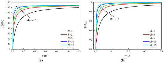
Figure 10.
Effect of parameter B on the proposed p–y curve. (a) p–y curve (b) normalized p–y curve.
4.2. Effect of Pile Diameter and Soil Depth on p–y Curve
The soil layer parameters are set as in Section 4.1, then different D values are set to investigate the effect of pile diameter on the shape of the p–y curve (A = 1, and B = 3). Figure 11a,b show the p–y curves and the normalized p–y curves for various D values. It can be observed from Figure 11a that the decrease in the soil stiffness (tangent modulus) becomes slower as the displacement increases and the ultimate lateral soil resistance becomes smaller as D increases. However, the normalized p–y curves for different pile diameters are completely consistent, as shown in Figure 11b.
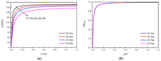
Figure 11.
Effect of pile diameter D on the proposed p–y curve. (a) p–y curve (b) normalized p–y curve.
Different z values are set to investigate the effect of soil depth on the shape of the p–y curve (A = 1, and B = 3). Figure 12a,b shows the p–y curves and the normalized p–y curves for various z values. As expected, the ultimate lateral soil resistance becomes larger and the increasing rate of decreases gradually as the soil depth increases, as shown in Figure 12a. However, the normalized p–y curves for different soil depths have an insignificant difference, as shown in Figure 12b. Hence, it can be approximately considered that the normalized p–y curve at different depths is unique.
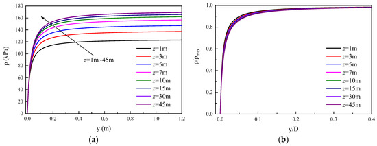
Figure 12.
Effect of soil depth z on the proposed p–y curve. (a) p–y curve (b) normalized p–y curve.
4.3. Validation of New p–y Formula
The normalized p–y curves corresponding to different depths for various pile diameters can be obtained according to the above 3D finite element analysis results, as shown in Figure 13. The proposed p–y curves (A = 1 and B = 3) and API p–y curves are plotted also in the figure. It can be observed that the proposed p–y curves can generally fit those obtained from 3D numerical simulation well. However, as a comparison, the API p–y curve significantly underestimates the soil stiffness. It should be noted that the proposed normalized p–y curve does not correspond to a specific soil depth, which is due to the fact that the soil depth has an insignificant effect on the shape of the normalized p–y curve, as described in Section 4.2 above. This comparison reflects the superiority of the proposed p–y curve over the API p–y curve.
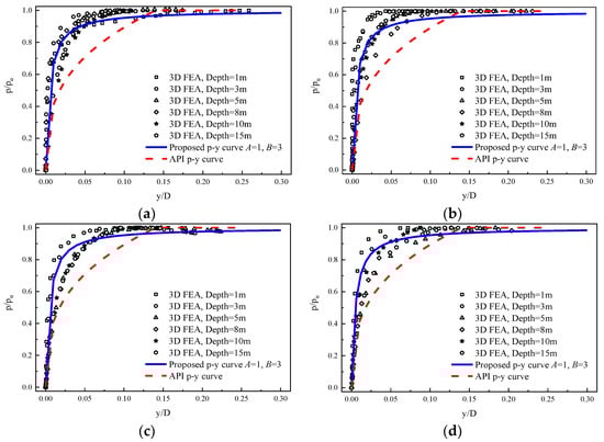
Figure 13.
Comparison of the proposed normalized p–y curves and those obtained from 3D numerical simulation. (a) Diameter = 1 m. (b) Diameter = 2 m. (c) Diameter = 3 m. (d) Diameter = 5 m.
The lateral responses of the piles with various diameters are predicted employing the BNWF method based on the proposed API p–y curve. The prediction results are compared with the 3D finite element results on Section 3.2, as shown in Figure 14. The prediction results including the load–displacement curve of the pile head, lateral deflection profile, and bending moment profile agree well with the 3D finite element results. This comparison demonstrates that, compared with API p–y curve, the proposed p–y curve can better predict the lateral behavior of piles in soft clays and has better applicability to large-diameter piles.
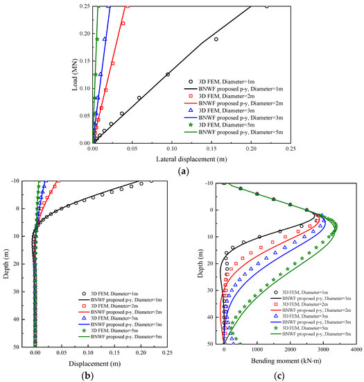
Figure 14.
Comparison of the lateral responses of piles obtained using the BNWF method (proposed p–y curve) and 3D finite element method. (a) Load–displacement curve of pile head. (b) Lateral deflection profile (c) Bending moment profile.
5. Summary and Conclusions
5.1. Main Conclusions
- (1)
- The BNWF method based on the p–y curve and 3D FEM for analyzing the lateral responses of monopiles are developed based on ABAQUS software and the accuracy of the two methods is validated using the field test results of the piles in soft clays.
- (2)
- The lateral responses of monopiles with different diameters are simulated by employing the two methods. It is found that the BNWF method based on the API p–y curve overestimates the deflection and bending moment while it underestimates the ultimate bearing capacity of the large diameter pile.
- (3)
- The API p–y curve significantly underestimates the ultimate soil reaction of soft clays and the degree of the underestimation increases as the soil depth increases; it also significantly underestimates the initial stiffness of the soft clays. These findings are supported by previous research results [12,15].
- (4)
- A new p–y model with variable parameters A and B was proposed that is more versatile and offers wider applicability to represent different soft clay and pile diameters. The current model can be simplified into the hyperbolic p–y model when A =1.
5.2. Significance and Application
As the most popular foundation type for supporting offshore wind turbines, large diameter monopile foundations must be designed for lateral loads such as winds, waves, and currents. The Beam on Nonlinear Winkler Foundation (BNWF) method has been widely used because of its clear concept and lower calculation cost. Compared with the three-dimensional finite element method, the BNWF method is easier to implement numerically. This method can be realized using ABAQUS software or, alternatively, by using other special calculation software for pile foundation such as LPILE or by compiling simple MATLAB programs. Hence, it has better applicability in engineering practice. The selection of a reasonable p–y curve is critical to the calculation accuracy of this method. This paper proposes a new p–y curve with better versatility and applicability. Compared with the API p–y curve, the proposed p–y curve can better predict the lateral behavior of piles in soft clays, such as the load–displacement curve of the pile head, lateral deflection profile, and bending moment profile, and has better applicability to large-diameter piles. However, it should be noted that the proposed p–y curve is mainly applicable to soft clay and not to other types of soil such as stiff clays and sands. When applied to engineering practice, the proposed p–y model can play a good role in the design of monopile foundations supporting offshore wind turbines in soft clays.
Author Contributions
Data curation, Q.L. and J.L.; Funding acquisition, M.W. (Mingyuan Wang); Investigation, M.W. (Mingyuan Wang) and J.L.; Methodology, M.W. (Mingyuan Wang), M.W. (Miao Wang) and X.C.; Resources, Q.L.; Software, M.W. (Miao Wang) and X.C.; Supervision, Q.L.; Validation, M.W. (Miao Wang); Writing—original draft, X.C. All authors have read and agreed to the published version of the manuscript.
Funding
This work was supported by the National Natural Science Foundation of China (52108334), the Natural Science Foundation of Tianjin City (20JCYBJC00570), and the Science and Technology Projects of Powerchina Huadong Engineering Corporation Limited (KY2020-KC-08-01-2021).
Data Availability Statement
The data presented in this study are available on request from the corresponding author. The data are not publicly available due to the follow-up research.
Conflicts of Interest
The authors declare no conflict of interest.
References
- Carter, J.M.F. North Hoyle offshore wind farm: Design and build. Proc. Inst. Civ. Eng.-Energy 2007, 160, 21–29. [Google Scholar] [CrossRef]
- Oh, K.Y.; Nam, W.; Ryu, M.S. A review of foundations of offshore wind energy convertors: Current status and future perspectives. J. Renew. Sustain. Energy Rev. 2018, 88, 16–36. [Google Scholar] [CrossRef]
- Wu, X.; Hu, Y.; Li, Y. Foundations of offshore wind turbines: A review. J. Renew. Sustain. Energy Rev. 2019, 104, 379–393. [Google Scholar] [CrossRef]
- Hamilton, B.; Battenberg, L.; Bielecki, M.; Bloch, C.; Decker, T.; Frantzis, L.; Paidipati, J.; Wickless, A.; Zhao, F. Offshore Wind Market and Economic Analysis: Annual Market Assessment; Navigant Consulting, Inc.: Burlington, MA, USA, 2013. [Google Scholar]
- Esteban, M.D.; Lopez-Gutierrez, J.S.; Negro, V.; Matutano, C.; Garcia-Flores, F.M.; Millan, M.A. Offshore wind foundation design: Some key issues. J. Energy. Resour. Technol. 2015, 137, 051211. [Google Scholar] [CrossRef]
- McClelland, B.; Focht, J.A. Soil modulus for laterally loaded piles. Trans. ASCE 1956, 182, 1–22. [Google Scholar] [CrossRef]
- Matlock, H. Correlations for design of laterally-loaded piles in soft clay. In Proceedings of the 2nd Offshore Technology Conference, Houston, TX, USA, 22–24 April 1970; p. 1204. [Google Scholar]
- API Recommended Practice 2GEO. Geotechnical and Foundation Design Considerations, 1st ed.; Addendum 1; American Petroleum Institute: Washington, DC, USA, 2014. [Google Scholar]
- Kondner, R.L. Hyperbolic stress-strain response: Cohesive soils. J. Soil. Mech. Found. Div.—ASCE 1963, 89, 115–143. [Google Scholar] [CrossRef]
- Georgiadis, M.; Anagnostopoulos, C.; Saflekou, S. Cyclic lateral loading of piles in soft clay. Geotech. Eng. 1992, 23, 47–60. [Google Scholar]
- Dewaikar, D.M.; Patil, P.A. A new hyperbolic p-y curve for laterally loaded piles in soft caly. Found. Anal. Des. 2006, 152–158. [Google Scholar]
- Jeanjean, P. Re-assessment of p-y curves for soft clays from centrifuge testing and finite element modelling. In Proceedings of the Offshore Technology Conference (OTC 20158), Houston, TX, USA, 4–7 May 2009. [Google Scholar]
- Klinkvort, R.T.; Hededal, O. Effect of load eccentricity and stress level on monopile support for offshore wind turbines. Can. Geotech. J. 2014, 51, 966–974. [Google Scholar] [CrossRef]
- Rathod, D.; Muthukkumaran, K.; Sitharam, T.G. Effect of slope on p-y curves for laterally loaded piles in soft clay. Geotech. Geol. Eng. 2018, 36, 1509–1524. [Google Scholar] [CrossRef]
- Zhu, B.; Zhu, Z.J.; Li, T.; Liu, J.C.; Liu, Y.F. Field tests of offshore driven piles subjected to lateral monotonic and cyclic loads in soft clay. J. Waterw. Port. C ASCE 2017, 143, 05017003. [Google Scholar] [CrossRef]
- Xu, D.S.; Xu, X.Y.; Li, W. Field experiments on laterally loaded piles for an offshore wind farm. Mar. Struct. 2020, 69, 102684. [Google Scholar] [CrossRef]
- Wang, Z.; Xie, X.; Wang, J. A new nonlinear method for vertical settlement prediction of a single pile and pile groups in layered soils. Comput. Geotech. 2012, 45, 118–126. [Google Scholar] [CrossRef]
- Zhang, C.; Yu, J.; Huang, M. Winkler load-transfer analysis for laterally loaded piles. Can. Geotech. J. 2016, 53, 1110–1124. [Google Scholar] [CrossRef]
- Choo, Y.W.; Kim, D. Experimental development of the p-y relationship for large-diameter offshore monopiles in sands: Centrifuge tests. J. Geotech. Geoenviron. Eng. 2016, 142, 04015058. [Google Scholar] [CrossRef]
- Boonyatee, T.; Lai, Q.V. A non-linear load transfer method for determining the settlement of piles under vertical loading. Int. J. Geotech. Eng. 2017, 14, 206–217. [Google Scholar] [CrossRef]
- Zhang, Y.; Andersen, K.H. Scaling of lateral pile p-y response in clay from laboratory stress-strain curves. Mar. Struct. 2017, 53, 124–135. [Google Scholar] [CrossRef]
- Elkasabgy, M.; El Naggar, M.H. Lateral performance and p–y curves for large-capacity helical piles installed in clayey glacial deposit. J. Geotech. Geoenviron. Eng. 2019, 145, 04019078. [Google Scholar] [CrossRef]
- Li, S.; Yu, J.; Huang, M.; Leung, C.F. Application of T-EMSD based p-y curves in the three-dimensional analysis of laterally loaded pile in undrained clay. Ocean. Eng. 2020, 206, 107256. [Google Scholar] [CrossRef]
- Zhang, Y.; Andersen, K.H. Soil reaction curves for monopiles in clay. Mar. Struct. 2019, 65, 94–113. [Google Scholar] [CrossRef]
- El Naggar, M.H.; Novak, M. Nonlinear analysis for dynamic lateral pile response. Soil Dyn. Earthq. Eng. 1996, 15, 233–244. [Google Scholar] [CrossRef]
- Gerolymos, N.; Gazetas, G. Phenomenological model applied to inelastic response of soil-pile interaction systems. Soils Found. 2005, 45, 119–132. [Google Scholar] [CrossRef]
- Allotey, N.; El Naggar, M.H. Generalized dynamic Winkler model for nonlinear soil-structure interaction analysis. Can. Geotech. J. 2008, 45, 560–573. [Google Scholar] [CrossRef]
- Heidari, M.; El Naggar, M.H.; Jahanandish, M.; Ghahramani, A. Generalized cyclic p-y curve modeling for analysis of laterally loaded piles. Soil Dyn. Earthq. Eng. 2014, 63, 138–149. [Google Scholar] [CrossRef]
- Liang, F.Y.; Chen, H.B.; Jia, Y.J. Quasi-static p-y hysteresis loop for cyclic lateral response of pile foundations in offshore platforms. Ocean Eng. 2018, 148, 62–74. [Google Scholar] [CrossRef]
- Wu, K.; Chen, R.; Li, S. Finite element modeling of horizontally loaded monopile foundation of large scale offshore wind turbine in non-homogeneity clay. IEEE Softw. 2009, 2, 329–333. [Google Scholar]
- Abdel-Rahman, K.; Achmus, M. Numerical modeling of the combined axial and lateral loading of vertical piles. In Proceedings of the 6th European Conference on Numerical Methods in Geotechnical Engineering, Graz, Austria, 6–8 September 2006; pp. 575–581. [Google Scholar]
- Haiderali, A.; Madabhushi, G. Three-dimensional finite element modelling of monopiles for offshore wind turbines. In Proceedings of the World Congress on Advances in Civil, Environmental and Materials Research, Seoul, Korea, 26–29 August 2012; pp. 3277–3295. [Google Scholar]
- Haiderali, A.; Cilingir, U.; Madabhushi, G. Lateral and axial capacity of monopiles for offshore wind turbines. Indian Geotech. J. 2013, 43, 181–194. [Google Scholar] [CrossRef]
- Cheng, X.L.; Wang, T.J.; Zhang, J.X.; Liu, Z.X.; Cheng, W.L. Finite element analysis of cyclic lateral responses for large diameter monopiles in clays under different loading patterns. Comput. Geotech. 2021, 134, 104104. [Google Scholar] [CrossRef]
- Achmus, M.; Abdel-Rahman, K.; Kuo, Y.S. Numerical modelling of large diameter steel piles under monotonic and cyclic horizontal loading. In Proceedings of the Tenth International Symposium on Numerical Models in Geomechanics, Rhodes, Greece, 25–27 April 2007; Taylor Francis: London, UK, 2007; pp. 453–459. [Google Scholar]
- Heidari, M.; Jahanandish, M.; El Naggar, H.; Ghahramani, A. Nonlinear cyclic behavior of laterally loaded pile in cohesive soil. Can. Geotech. J. 2014, 51, 129–143. [Google Scholar] [CrossRef]
- Hong, Y.; He, B.; Wang, L.Z.; Wang, Z.; Ng, W.W.C.; Masin, D. Cyclic lateral response and failure mechanisms of semi-rigid pile in soft clay: Centrifuge tests and numerical modelling. Can. Geotech. J. 2017, 54, 806–824. [Google Scholar] [CrossRef]
- He, B.; Lai, Y.; Wang, L.; Hong, Y.; Zhu, R. Scour effects on the lateral behavior of a large-diameter monopile in soft clay: Role of stress history. J. Mar. Sci. Eng. 2019, 7, 170. [Google Scholar] [CrossRef]
- Dassault Systemes Simulia Corp. Abaqus Analysis User’s Manual Version 6.14; Simulia: Johnston, RI, USA, 2014. [Google Scholar]
- Murff, J.D.; Hamilton, J.M. P-ultimate for undrained analysis of laterally loaded piles. J. Geotech. Eng. 1993, 119, 91–107. [Google Scholar] [CrossRef]


Publisher’s Note: MDPI stays neutral with regard to jurisdictional claims in published maps and institutional affiliations. |
© 2022 by the authors. Licensee MDPI, Basel, Switzerland. This article is an open access article distributed under the terms and conditions of the Creative Commons Attribution (CC BY) license (https://creativecommons.org/licenses/by/4.0/).