Abstract
The rapid economic development (ED) of the Yangtze River Economic Belt (YREB) has had a significant negative impact on regional ecosystem services (ES). Accurately understanding and properly handling the relationship between ES and ED is critical to achieving coordinated regional development of the YREB. Restricted by a minimal number of research units, traditional studies have not fully considered the spatial heterogeneity of the influencing factors, leading to results with poor accuracy and applicability. To address these problems, this paper introduces a spatial econometric model to explore the impact of influencing factors on the level of coordinated development in the YREB. For the 1013 counties in the YREB, we used the value equivalent method, the entropy weight method, and the coupling coordination model to quantify the coupling coordination relationship between the ecosystem services value (ESV) and ED from 2010 to 2020. The multi-scale geographically weighted regression model (MGWR) was adopted to analyze the role of influencing factors. The results showed the following: (1) The coupling coordination degree (CCD) of ESV and ED along the YREB demonstrated significant spatial heterogeneity, with Sichuan and Anhui provinces forming a low-value lag. The average CCD from high to low were found in the Triangle of Central China (TOCC), the Yangtze River Delta urban agglomeration (YRDUA), and the Chengdu–Chongqing urban agglomeration (CCUA). (2) There was spatial autocorrelation in the distribution of CCD, with high–high clustering mainly distributed in Hunan, Jiangxi, and Zhejiang provinces. The counties with high–high clustering were expanding, mainly centering on Kunming City in Yunnan Province and expanding outward. (3) There was significant spatial heterogeneity in the impact of each influencing factor on CCD. Per capita fiscal expenditure was sensitive to low–low clustering areas of CCD; per capita, food production was a negative influence, and the rate of urbanization transitioned from negative to positive values from west to east.
1. Introduction
The ecosystem is the material basis for meeting the essential requirements for the survival and development of humanity. It is central to the sustainable development of regions and countries. The rational use of ecosystems for economic development can contribute to regional economies, but overexploitation can seriously damage ecosystem integrity. With the rapid development of China’s economy, problems such as deterioration of the ecological environment, frequent natural disasters, and significant regional economic disparities have become increasingly prominent [1,2,3]. Therefore, accelerating the implementation of coordinated regional development has become a significant national strategy [4]. The YREB is a central strategic development region in China. In the last few years, the rapid economic growth and urbanization of the YREB induced huge consumption of natural resources and degradation of the ecosystem [5], which restricted its sustainable development [6]. “The 14th Five-Year Plan” makes proposals to comprehensively promote the development of the YREB and coordinate protection of the ecological environment and economic development. Protecting the YREB’s ecological environment, rather than carrying out low-quality economic development, has become the key focus of the country’s river development plans [6,7]. Therefore, objectively and accurately evaluating the development status of the ecosystem and economic system, clarifying the intrinsic relationship between them, and exploring the correct development path have become challenging hot topics in academic research. It is a critical path to achieving high-quality development in China. Related studies have shown that there are many other large watersheds in developing countries in the world, such as the Ganges River Basin and the Amazon River Basin, with similar problems, such as prominent human–land conflicts and polluted ecological environments [8,9]. This study will provide sustainable development ideas for these regions of ecological and economic imbalance. It also provides a theoretical and practical basis for the green and healthy evolution of other developing countries.
Ecosystem Service Values (ESV), as core indicator of ES [10], have been highly valued by academics since the early 1990s. ESV represents the total value of the various benefits humans derive from ecosystems [11]. Implementation of UN Millennium Ecosystem Assessment Project has made more scholars recognize the importance of ES, which plays a significant role in human survival and sustainable socio-economic development. As a consequence, research on relation ecosystem service functions, values, and drivers has been promoted [12,13,14]. In current studies, some scholars have quantitatively assessed the values of single ES in the study area [15,16], including soil and water conservation and water use [17]. Some scholars have also used the value-equivalent method to measure the ecological value of land in the study area from the perspective of land value [18]. This is a simple and efficient method for assessing ecological value on a large scale and is therefore mainly used in empirical studies [19]. ESV is the value expressions of the utility of ES and can quantify the service functions of natural ecosystems [20]. ESV are also closely related to land use change, which is a crucial factor affecting global environmental change [21]. Therefore, using ESV to evaluate the degree of development of natural ecosystems can accurately reflect the evolution of regional ecosystem quality and the impact of human social production activities on the ecosystem [22].
As early as the 1990s, Grossman et al. [23] proposed the theory of Kuznets curve (EKC), which states that the relationship between economic growth and environmental pollution is not linearly correlated, but rather an inverted “U” shape. It is believed that the impact of ED on the environment involves initial deterioration followed by later improvement. Research into the relationship between the socio-economic development and ecology in China started late, but, since the 1980s, the issue of coordinated socioeconomic and ecological development has gradually received more attention from an increasing number of scholars [24]. To better measure the linkages and synergistic evolution of ecological and socio-economic development, assess the status of the human–Earth relationship, and achieve coordinated regional development, the use of quantitative research methods to analyze the collaborative relationship between ecology and economy has gradually become a key research direction [25]. There is an inherent need for coordinated development because the regional economy and natural environment can benefit each other in a coupled and coordinated co-development process. The coupling effect and CCD have now become an effective research tool for the evaluation of the overall balanced development of a region or society’s levels of coordination and development [26], and it is widely used in the research into ED and the ecological environment [27,28], ES and urban development [29], urbanization and the eco-environment [30,31]. Most of the studies have focused on the large, national [32], river basins [27], urban agglomeration [33], and provincial areas [34].
Many studies considered the relationship between ESV and ED. With regard to research scale, Yanni Cao et al. [35] studied the relationship between provincial ESV and ED in China from three dimensions (nationwide, eastern, central, and western regions, and provincial administrative regions). Wanxu Chen et al. [25] studied the relationship between ESV and ED in Hunan Province at county scale. At present, there are few studies on county ESV and ED in large economic belts. China is a vast country with significant spatial heterogeneity. There are differences in the distribution of economic and ecological development, even within the same provincial and municipal administrative regions. Therefore, precise research is required to assess the ESV and ED at county level, and this could improve the accuracy and reliability of results. From the perspective of influencing factors, many studies have only focused on time-series changes or spatial–temporal distribution characteristics of the relationship between ESV and ED and given less attention to analysis of the influencing factors. In recent years, however, continuous attention has been given to the analysis of factors that influence the development of coupling coordination relationships. Most studies have used the multivariable linear regression model [36], geographic detector model [37], panel Tobit econometric model [38], etc., but few studies have made use of spatial econometric methods to analyze factors influencing the relationship between ESV and ED. By introducing a spatial econometric model, this paper is able to fill the MGWR gap for the study of the coupling coordination relationship between ESV and ED at small levels in the large economic belt.
Based on this, our study took the county (district) unit of the YREB as the research object and constructed its ecology–economy coupling coordination system. We selected spatial autocorrelation analysis tools, incorporated the multi-scale geographically weighted regression model (MGWR) in the analysis of the drivers of the ecology–economy coupling coordination relationship, and then analyzed the coupling coordination for each region of the YREB at different periods. The spatial variation of the CCD and the specific spatial effects of the factors influencing the CCD were analyzed. Through the scientific and objective evaluation system, we searched for the inner logic of the ecology–economy coordinated development of the YREB, explored the path of their coordinated development, and identified the relevant external drivers to provide a theoretical basis for a coordinated development policy for the YREB and other regions.
This study aimed to address the following issues:
- (1)
- To evaluate the number distribution characteristics of the coupling coordination relationship between the ESV and ED of the YREB and its three major urban clusters from 2010 to 2020.
- (2)
- To analyze the spatiotemporal evolution characteristics of the coupling coordination relationship between the ESV and ED of the YREB from 2010 to 2020.
- (3)
- To measure the spatial autocorrelation relationship between the ESV and ED in the YREB from 2000 to 2020.
- (4)
- To explore the spatial heterogeneity of the effect of different influencing factors on CCD in the YREB from 2000 to 2020.
2. Study Area
The YREB (Figure 1) spans three regions in the east and west of China and three terrains of landforms, covering 11 provinces and cities, including Shanghai, Jiangsu, Zhejiang, Anhui, Jiangxi, Hubei, Hunan, Chongqing, Sichuan, Guizhou, and Yunnan, with a total area of about 2.05 million square kilometers. By 2020, the regional GDP of the YREB reached 47.16 trillion yuan, and the resident population reached 548 million, respectively, accounting for 46.4% and 37.96% of the total for the country, making this a significant area of economic growth and population concentration in China. The region has three major city clusters: the Yangtze River Delta urban agglomeration (YRDUA), the Triangle of Central China (TOCC), and the Chengdu–Chongqing urban agglomeration (CCUA). The three major urban agglomerations radiate from the central cities and create three major poles of growth in the YREB. The three major urban agglomerations make significant contributions to the overall ED of the YREB. The YREB is a vast area with considerable differences in natural resource endowments and socio-economic conditions across its districts and counties. The natural environment in the region has been damaged to different degrees since the last century. At the same time, the coordinated development of ecology and economy faces a severe challenge because of the imperfect mechanism for coordination of regional development and the imbalance in regional development levels. Therefore, reducing the scale of the study areas to the county units for quantitative analysis of the coupling coordination relationship between ES and ED will benefit coordination of regional development and the construction of an ecological civilization.
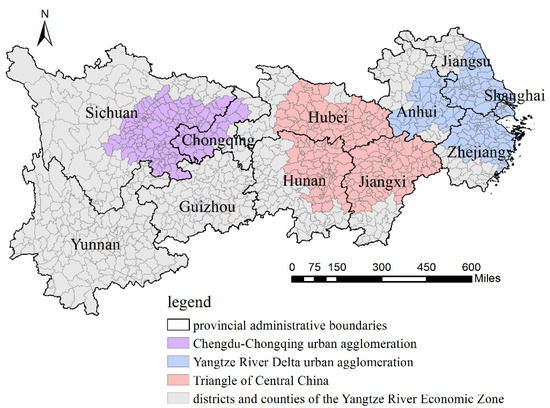
Figure 1.
Regional overview of the YREB.
3. Methods and Data Sources
3.1. Methods
3.1.1. Construction of the Economic Development Index System
The construction of the evaluation index system followed the principles of systematicity, scientificity, accessibility, and representativeness, and this study referred to existing studies [39,40,41,42] to construct the social development evaluation index system. The indicators in Table 1 were selected from the three dimensions of ED: scale, quality, and structure. These indicators were used to support the rationality of the selection of the ED evaluation index system.

Table 1.
Composition and weights of ED evaluation index system.
Scale of ED
This century is characterized by a changing distribution of GDP per capita growth rates, which is reflected in different shapes and a persistent asymmetry at the regional level and for countries at different development levels [43]. The YREB is the economic belt with the highest level of ED and the strongest overall competitiveness in China, and the YREB’s GDP accounted for 46.42% of the entire Chinese GDP in 2020. The GDP of the YREB varies widely, with the GDP of each province gradually decreasing from east to west, and there is strong spatial heterogeneity among the counties within each province. According to Zhiqiang Jiang’s study, the key to measuring regional ED is the GDP and its growth rate [44]. To exclude the effect of population size, this paper used GDP per capita as an indicator to evaluate the scale of ED.
According to Sorana Vatavu et al., taxes are important instruments for governments and should be used for economic growth [45]. Local fiscal revenue reflects the revenue capacity of local governments, and generally regions with higher local fiscal revenue have larger economies. Therefore, this study selected local fiscal revenue per capita as another key indicator to measure the scale of ED.
Quality of ED
The quality of ED in the YREB was determined using two indicators: social fixed asset investment per capita (yuan/person) and retail sales of social consumer goods per capita (yuan/person). The reasons for choosing social fixed asset investment per capita are as follows: on the one hand, fixed asset investment can be directly converted into productivity and promote economic growth in the short term. On the other hand, the YREB is currently facing a serious dilemma concerning industrial upgrading, and fixed asset investment is an important driver for the transformation and upgrade of manufacturing industries [46], which can effectively contribute to high-quality economic development. Therefore, this paper selected social fixed asset investment as an indicator to measure the quality of economic development. Due to the large population disparity among counties, social fixed asset investment per capita (yuan/person) was used for the study.
The reasons for selecting retail sales of social consumer goods per capita were as follows: The total retail sales of consumer goods is not only an important indicator to measure the consumption level of the Chinese people, but also an important indicator of the healthy development of the national economy [47]. Retail sales of social goods measure the level of economic activity within a region from the perspective of consumer spending. There are more than 1000 counties in the YREB, and there are large disparities in the consumption capacity of the population between counties, so the per capita retail sales of social goods were used as an indicator of the quality of economic development in the region.
Structure of ED
According to the Petty–Clark Theorem, as economic development and the level of national income per capita increase, there is an evolutionary trend of the labor force shifting first from primary industry to secondary industry and then to tertiary industry [48]. From 2010 to 2020, the YREB experienced industrial transformation and industrial upgrading, and the ratio of its secondary industry to tertiary industry changed from 38.74:54.02 to 49.69:41.08, which is a very drastic change. Therefore, the simultaneous introduction of secondary and tertiary industries can be used as an indicator to reflect the ED structure of the YREB in a more targeted way.
3.1.2. Ecosystem Service Value Assessment Methods
Based on the terrestrial ESV per unit area equivalent factor table developed by Gaodi Xie et al. [18,49], one standard unit ESV equivalent factor is defined as 1/7 of the annual economic value of the natural food production of farmland with an average yield of 1 hm2 [50,51]. We utilized this method to calculate ESV in the study area, and corrected ESV using the consumer price index (CPI) in conjunction with related research [52]. The level of ecosystem development in each county (district) was measured using the land-average ESV according to the following formula.
In Formulas (1) and (2), is the economic value of food production per unit area of farmland ecosystem (yuan), is the average price of food crops (yuan), is the yield per unit area of food crops (kg/hm2), is the equivalent value of ES per unit area (yuan), and is the value of ES per unit area.
In Formulas (3) and (4), is the regional value of ES, is the area of the th land use type (hm2). is the unit area value of the first land use type (yuan), and is the county (district) area land-average ecosystem service value. The corrected ecosystem service values per unit area of the YREB are shown in Table 2.
Table 2.
ESV per unit area of YREB (Yuan/hm2).
3.1.3. Measurement of Coupling Degree
Coupling refers to a phenomenon whereby two or more systems affect each other through various links or effects. When the elements within or between systems act positively, cooperating and developing in a coordinated way, it is called benign coupling, and vice versa [38]. The degree of coupling is a specific value which reflects the strength of interaction between different systems but cannot reflect the level of coordination between those systems. It is therefore necessary to introduce a degree of coupling coordination model to quantify the coordination between ecological and economic development systems. The specific formula is as follows.
In Formula (5), is the CCD, and the more extensive the value, the higher the level of coordinated development between the two systems, whereas a smaller value indicates a lower level of coordination [53]; represents the coupling degree, with larger values indicating greater coupling of the two systems and the smaller values, lower levels of coupling.
In Formulas (6) and (7), is the standardized level of development of ecosystem service values, is the level of the standardized ED index system, and is the sum of the integrated evaluation index of the ecosystem and economic system. Coefficients and are to be determined, and this paper assumed that the two subsystems were equally important, with both values at 0.5 [25]. The distribution function created by Chongbin Liao [54] was used to determine the CCD classification criteria (Table 3).
Table 3.
Classification of coupling coordination level of YREB.
3.1.4. Analysis of Autocorrelation
The use of spatial autocorrelation analysis makes it possible to portray the spatial characteristics of the collaborative ecological–economic development of the study area. Global autocorrelation was used to evaluate the overall spatial dependence of all units in the study area, which was measured in this paper using the global Moran’s I index with the following Equation.
In Formula (8), is the number of cells in the space, and represent cells and of observations, is the spatial weight array based on the spatial , the spatial weight array established by the adjacency relation, is the mean value, and is the standard deviation.
In order to further reflect the local instability of spatial autocorrelation and analyze the aggregation and divergence characteristics of local cells, local Moran’s I was introduced, and its specific formula is:
According to the spatial characteristics of the distribution of ecology–economy coupling coordination in the YREB, the local Moran’s–I–index can be divided into four types of aggregation: high–high, low–low, high–low, and low–high. High–high agglomeration indicates that counties (districts) with high CCD are surrounded by counties (districts) with high CCD, high–low agglomeration indicates that counties (districts) with high CCD are surrounded by counties (districts) with low CCD, low–high agglomeration indicates that counties (districts) with low CCD are surrounded by counties (districts) with high CCD.
3.1.5. Multiscale Geographically Weighted Regression (MGWR)
The MGWR was proposed by Fotheringham in 2017 [55]. This paper used MGWR to explore how the drivers influenced the ecological–economic coupling coordination in the YREB at the spatial level. Compared with the traditional multiple linear regression model (OLS), the classical geographically weighted regression model (GWR) introduces a spatial distance weight matrix, and its evaluation results are more reliable at spatial scales. GWR has the same bandwidth for all variables and does not allow different spatial smoothing levels for each variable, whereas MGWR applies different bandwidths to measure the geospatial scale of action of the explained variables affected by the explanatory variables. Compared to the GWR, MGWR is more consistent with the spatial heterogeneity of geographic processes and is calculated as follows.
In Formula (10), is the explanatory variable, is the first explanatory variable, denoting the local parameter estimate of the kth explanatory variable of sample denoting sample , is the bandwidth used for the regression coefficient of the jth variable, represents the coordinates of the spatial unit , is the regression coefficient of the explanatory variable, and is the random error.
3.2. Data Sources
In this study, remote sensing detection data of current land use in China for 2010, 2015, and 2020 at 30 m resolution were provided by the Resource and Data Science Center of the Chinese Academy of Sciences (https://www.resdc.cn/ (accessed on 1 July 2022)). They were resampled to 100 m resolution and reclassified into seven land use types (farmland, forest land, grassland, water area, construction land, barren land, and wetland) for ecosystem service value calculation. The production, area, and price of significant grains (rice, wheat, corn, and soybean) were in the ecosystem service value equivalent. The consumer price index (CPI) data used in the correction of the identical factor were obtained from the China Statistical Yearbook and the China Agricultural Price Survey Yearbook. Elevation data were derived from (http://www.gscloud.cn/ (accessed on 1 July 2022)), using SRTMDEMUTM 90M data. Annual average temperature, rainfall, and potential evapotranspiration data were obtained from meteorological observation data (http://data.cma.cn/ (accessed on 1 July 2022)) using the Kriging interpolation method to process data from each meteorological station to calculate the annual average temperature, rainfall, and potential evapotranspiration of the whole region. NDVI data were obtained from (https://www.resdc.cn/ (accessed on 1 July 2022)). PM2.5 data were obtained from (http://www.geodata.cn (accessed on 1 July 2022)). Finally, socio-economic data were obtained from the China County Statistical Yearbook, provincial and municipal statistical yearbooks, and published statistical bulletins on national economic and social development.
4. Results
4.1. Comprehensive Development of the Ecological-Economic System
As shown in Table 4, the overall coupling coordination of the YREB improved from 2010 to 2020. The overall mean value of 1013 study units increased from 0.4678 to 0.4872, which was on the verge of disorder. The extreme value showed a positive trend (both the maximum and minimum values showed different degrees of increase). The coupling coordination level of the YREB showed a trend of “shrinking disorder and expanding coordination” over 10 years, in which the proportion of near-disorder decreased significantly (from 59.62% to 45.61%) and the proportion of barely coordinated increased significantly (from 27.05% to 46.59%). Specifically for the county (district) study unit, Changning District in Shanghai was the lowest coupling coordination area in 2010 and 2020 and was in moderate dissonance; Junshan District in Yueyang City, Hunan Province; Shiyan City, Hubei Province; and Shengsi County in Zhoushan City, Zhejiang Province were the highest coupling coordination areas in 2010, 2015, and 2020, with values of 0.6429, 0.5989, and 0.7114, respectively.
Table 4.
Measurement results of the CCD of the YREB and the three major urban agglomeration.
The CCDs of the different urban agglomerations varied significantly. The YRDUA, the TOCC, and the CCUA had 176, 216, and 141 counties (districts) which were primary research units, respectively. Then, the quantitative characteristics of their CCDs were counted. The percentage of disorder (or coordination) units reflected the dynamic changes in CCD among the three major urban agglomerations in different periods. The overall CCD of the urban agglomeration in the TOCC was higher than that of the YRDUA and the CCUA over 10 years. In addition, the TOCC had the highest percentage of barely coordinated regions. It has become the region with the best degree of ecological–economic coupling and coordinated development. The proportion of imminent disorder and barely coordinated in the TOCC changed significantly, with the proportion of imminent disorder decreasing from 50.93% to 30.09%, a decrease of 20.84%, and the proportion of barely coordinated increased from 43.06% to 67.59%, an increase of 24.51%. The proportion of areas on the verge of disorder in the CCUA was high, reaching 70.92% in 2020, whereas the proportion with mild disorder was decreasing year by year, and ecological–economic coupling and coordinated development has improved. It is worth noting that the characteristics of the three major urban agglomerations were different, with the YRDUA having the best degree of coupling and coordination. In addition, the TOCC had no moderate disorder unit and the CCUA had no prior coordination unit.
4.2. Temporal and Spatial Coupling Coordination Characteristics of the Ecological–Economic System
We compared the CCD trend of county (district) units in the YREB during the ten- year period, and the results are shown in the Figure 2. We identified three main distribution characteristics. The first was that the CCD increased from west to east and from south to north in an “inverted U” distribution. The second was that the spatial heterogeneity of the CCD decreased year by year. The third was that the slope of the trend line in both the east–west and north–south directions decreased. These distribution characteristics indicate that the coordinated development concepts and policies of the YREB were intensifying, and synergistic development was achieving significant results within that period
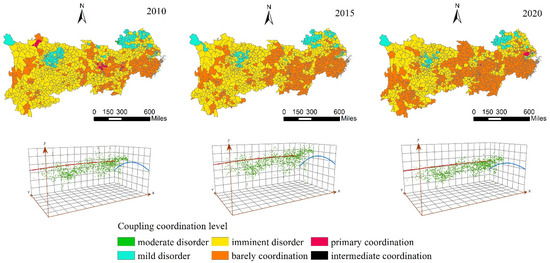
Figure 2.
Spatial and temporal distribution and trend surface analysis of ecological–economic coupling coordination by county units in the Yangtze River Economic Zone.
As shown in Figure 2, Zhejiang Province was the province with the best ecological–economic coupling coordination development. The border of Zhejiang, Anhui, and Jiangxi Provinces was the densest area with a high CCD in the whole economic belt. A large number of counties (districts) with low CCD existed in northern Jiangsu Province and central and western Sichuan Province. Among the remaining regions, Jiangxi, Hunan, and Hubei Provinces had high coupling coordination, and most districts and counties in their territories had a CCD higher than 0.479, nearly reaching barely coordinated.
The coupling coordination level in Sichuan Basin was low. A large number of central counties (districts) such as Jinyang City, Jintang County, Neijiang City District, and Ziyang City District were showing mild disorder, which was a fundamental reason for the low CCD of the CCUA. Most counties (districts) in Yunnan Province had developed rapidly in terms of coupling coordination, with counties in the Chuxiong Yi Autonomous Prefecture and Jinghong City in Xishuangbanna Dai Autonomous Prefecture, urban Kunming, Jingdong Yi Autonomous Prefecture in Pu’er City, and counties (districts) in Yuxi City being fully developed. They were the most changed areas in the YREB. It was noteworthy that the coupling coordination level of Suzhou City in Jiangsu Province had steadily increased from 2015 to 2020 based on an initially high CCD. Zhejiang Province had the largest concentration of barely coordinated with balanced and high-quality ecological–economic development, and the variability of its CCD continued to narrow and began to spread to surrounding provinces in 2020.
4.3. Spatial Autocorrelation Analysis of the CCD of the YREB
The global Moran’s I value of ecological–economic coupling coordination in each county (district) from 2010 to 2020 was calculated according to Formula (8) with the help of the spatial statistical analysis tool in GeoDa software. The Moran’s I values for 2010, 2015, and 2020 were 0.447, 0.452, and 0.461, respectively, and all of them pass the significance test at the 1% level, indicating that the spatial distribution of ecological–economic CCD in the counties (districts) of the YREB was not randomly distributed. Instead, it showed that the spatial distribution of the CCD in certain counties (districts) of the YREB tended to cluster in space. In addition, the increasing trend of Moran’s I value from 2010 to 2020 indicated that the spatial aggregation of the study units in the YREB was increasing.
We used local spatial autocorrelation analysis according to Formula (9) to analyze the spatial autocorrelation existing between different counties (districts) and finally obtain the LISA clustering map (Figure 3). The number of counties (districts) passing the 1% significance test for local Moran’s I in the YREB in 2010, 2015, and 2020 were 682, 703, and 735, accounting for 67.32%, 69.40%, and 72.56% of the total study units, respectively, an increase of 7.71% over the decade, which indicated that more and more research units with similar coordination levels were tending to cluster. We can see that the number of high–high and low–low clusters was increasing, whereas the number of low–high and high–low clusters was less changeable. The number of high–high clusters increased by 14.88% in ten years, forming an evolution pattern of “high–high clusters expanding, other clusters holding steady”. This evolution pattern indicates that the ecological–economic coupling is continuously improving, which verifies the previous conclusion. With regard to spatial distribution, the high–high clusters were mainly concentrated in Hunan, Jiangxi, and Zhejiang provinces. They were distributed more closely in concentrated continuous blocks, whereas the low–low clusters were mainly concentrated in Sichuan, Anhui, and Jiangsu provinces.
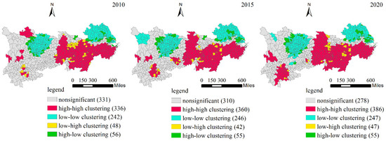
Figure 3.
LISA map of the coupling coordination of the YREB, 2010–2020.
In terms of time, the main changes in clustering from 2010 to 2020 were concentrated in Yunnan, Hubei, and Sichuan Provinces. High–high clustering changes were the most obvious in Yunnan Province, with a number of clustered insignificant areas evolving into high-value aggregation areas. In Chuxiong Yi Autonomous Prefecture, Yuxi City, Honghe Hani Yi Autonomous Prefecture, and Pu’er City of Yunnan Province, there were many non-significant clustering areas that were transformed into high–high clustering areas. This indicates that in recent years, Yunnan Province has relied on its location to vigorously develop tourism to promote ED, while also protecting the ecological environment. Coupled with the policy advantages adopted by the state to actively drive shared prosperity, this has created a positive situation of high-value CCD aggregation which has spread outward over time. It is worth noting that most counties (districts) which experienced a significant shift in clustering were better endowed in terms of the natural environment but had a weaker economic base. These counties (districts) had made full use of their characteristics during the decade in which China’s economic model shifted from being export-oriented and labor-intensive to investment-oriented and capital-intensive. These counties (districts) promoted the concept of sustainable development to encourage the growth of tertiary industries that would eventually achieve coordinated ecological–economic development.
4.4. Analysis of Influencing Factors Based on MGWR
4.4.1. Variable Selection
Based on the availability of data and the synthesis of existing studies, this paper selected rainfall (in mm), potential evapotranspiration (in mm), temperature (in °C), and relief amplitude (in m) as natural drivers of CCD, and the NDVI as the initial data sources [56]. Per capita financial expenditure (million yuan/person), population density (unit: person/km2), PM2.5 concentration (unit: um), per capita food production (unit: t/million), and urbanization rate (unit: %) were selected as social drivers of CCD [37,57,58]. Rainfall, potential evapotranspiration, and temperature were the annual average values of the region. The relief amplitude was calculated as the difference between the maximum and minimum elevation values of all the image elements in the unit. NDVI referred to the normalized vegetation index, which was used to reflect natural plant and crop growth. The per capita fiscal expenditure was calculated from the ratio of the amount of local fiscal expenditure to the resident population, to measure the scale of fiscal expenditure. PM2.5 referred to delicate particulate matter (the higher its concentration, the worse the air quality), which can be used to measure the degree of human pollution of nature. Per capita food production was calculated from the ratio of total food production to resident population and the urbanization rate was calculated from the ratio of the area of built-up land to total area.
4.4.2. Model Comparison
We used different models to calculate the impact of each driver on the coupling coordination in 2010, 2015, and 2020. The statistical results for these three years were averaged as a comparison and the results are shown in Table 5. The fit of the MGWR was better than the OLS and GWR models, and the AICc value was also the lowest, so it could be concluded that the results from the MGWR were better than the other two models. In addition, the number of effective parameters and the sum of squared residuals were smaller for the MGWR, indicating that the model is able to obtain more accurate regression results using fewer parameters.
Table 5.
Regression results of OLS, GWR, and MGWR.
4.4.3. Scale Analysis
From a comparison of the GWR and MGWR bandwidths (Table 6), it was found that the MGWR could fully reflect the bandwidths of different driver effects and express the spatial heterogeneity more accurately, providing results that were closer to the natural spatial processes. In contrast, the GWR could only reflect the average value of the driver effect scales. The bandwidth of the GWR was 86, accounting for 8.49% of the total number of cells, whereas the scale of action of the different drivers of the MGWR varied widely. Through the MGWR calculation, it was found that there were a large number of areas with insignificant regression coefficients for the four variables, and these were rainfall, potential evapotranspiration, PM2.5 concentration, and population density. Although some variables in the results were insignificant in local areas, such as NDVI, temperature, relief amplitude, per capita fiscal expenditure, per capita food production, and urbanization rate, there were more significant areas overall, which explained the changes in coupling coordination from a spatial perspective. Finally, the variables of rainfall, potential evapotranspiration, PM2.5 concentration, and population were excluded from further analysis.
Table 6.
GWR and MGWR bandwidth for each influencing factor.
The constant indicates the influence on the CCD resulting from different geographical locations under the condition that other driving factors are determined, and it reflects the overall influence on the CCD of other influencing factors such as the strength of environmental protection and economic structure that are not considered in this paper. The constant works on a scale of 416, accounting for a more significant proportion of all cells and indicating that other influencing factors had a more extensive influence on the CCD, with lower spatial heterogeneity and smoother coefficient distribution in space. The NDVI value had the least effect on the CCD, at only 44, which accounted for 4.34% of the total number of cells. This indicated that the NDVI value had a similar effect on the CCD in half of the province, but its effect changed dramatically when the range exceeded half of the province. It also indicated that the CCD was more sensitive to changes in the NDVI value. The action scale of temperature was 936, which was almost the global scale, indicating that although temperature affected the coupling coordination, the difference in its effect on each location was minimal, and there was almost no spatial heterogeneity. The action scale of relief amplitude was also minor at 88, almost reaching the local scale, indicating significant spatial heterogeneity in the influence of topographic factors on the CCD. The per capita fiscal expenditure effect scale was 148, which corresponded to the local scale range of one central province, accounting for 14.61% of the total sample size, and indicating that there was spatial heterogeneity between provincial size ranges in terms of its effect on the CCD. The effects of per capita food production and urbanization rate on coupling coordination were 64 and 59, respectively, which belong to a small range scale, indicating that both effects on coupling coordination varied widely from a spatial perspective and that the coefficients were more unstable.
4.4.4. Spatial Heterogeneity Analysis of Drivers
Since the multi-scale geographically weighted regression model was applied to cross-sectional data, the YREB data from 2010 to 2020 were averaged to obtain the average magnitude of the contribution of each driver to the coupling coordination over the decade and to enable the representation to be visualized. The MGWR results reflected the magnitude of the effect of a driver on the dependent variable for each study unit locally, and there could be problems if a driver had a significant effect on the dependent variable globally but not locally for the unit. Ignoring the local significance would make the research results lose their practical significance, so this study used the local p-value size to verify whether the local influence factors significantly impacted the coupling coordination and set values below 0.05 as significant. Units with other values were considered nonsignificant.
As shown in Figure 4, there was an obvious pattern of spatial ladder distribution. The coefficients constantly decreased from west to east and the high values were mainly concentrated in the coastal provinces. This means that under the condition that the driving factors were determined in this paper, the influence of other driving factors on the CCD was more significant in the east than in the center of the study area. Factors such as the strength of environmental protection and economic structure that were not considered in this paper had a more significant influence on the CCD in the eastern region of the YREB. This may be because of the higher level of socio-economic development in the eastern region of the YREB, where social drivers (e.g., per capita fiscal expenditure, urbanization rate) have reached a higher level and have less impact on the economic system, and where the natural drivers have little overall impact on the ecosystem because of internal offsetting (for example, the influence direction between NDVI and fluctuation amplitude is inconsistent). Therefore, our results indicated that, the economy and ecosystem were less affected by the selected driving factors and were sensitive to other influencing factors.
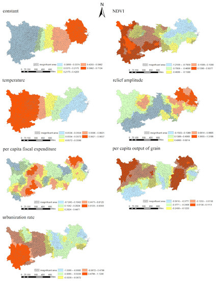
Figure 4.
Spatial heterogeneity of each influencing factor of ecological–economic coupling coordination in the YREB.
The NDVI had both positive and negative effects on coupling coordination, and its lower negative coefficient was mainly distributed in the dense farmland areas in the east. In comparison, its higher positive coefficient was mainly distributed in the Dali Bai Autonomous Prefecture and Lijiang City in Yunnan, which have excellent natural environmental conditions. The main reason for the inconsistent influence direction is that the NDVI value only reflects the vegetation cover. The ecological base of Yunnan Province was better than in other provinces, and there is still much room for ecological development, so the increase in the NDVI value will continue to promote improvement of ESV in the region, thus increasing the coupling coordination. An increase in the number of crops also promotes higher NDVI. The higher NDVI values seen in Anhui, Jiangsu, and Hubei provinces may be a manifestation of crop density, which is not conducive to ecosystem service development. Therefore, our results indicated that the increase in NDVI instead reduced the ESV per unit area, further reducing the coupling coordination of the initially more fragile ecosystems in the grain-growing areas of Jianghuai. In addition, we found that the CCD of Zhejiang and Jiangxi provinces was less affected by the NDVI values than Anhui and Jiangsu provinces, because Zhejiang and Jiangxi have relatively less farmland. Hence, the reduction in ecosystem service value per unit area was relatively small.
The effect of temperature on the CCD was minor, the regression results of temperature were significant, and there were almost no nonsignificant cells. From the coefficients, it can be seen that there was very little spatial heterogeneity of temperature on coupling coordination, and its effects on coupling coordination were all positive and decreased gradually from the west to the east, indicating that temperature had limited impacts on the development of coupling coordination.
The influence of relief amplitude on the CCD was positive, and the higher degree of influence was mainly in the plains because the ecological environment in the plains was more vulnerable to human damage, which leads to an increase in the ESV in line with the relief amplitude. In cases of the same economic level, increasing the ecological level will increase the coupling coordination.
Fiscal expenditure per capita positively affected coupling coordination, and the regions with negative coefficient values were mainly nonsignificant. There was significant spatial heterogeneity in the impact of per capita fiscal expenditure on coupling coordination, with higher coefficients in the urban agglomerations of Sichuan and Chongqing, eastern Yunnan Province, western Guizhou Province, northern Zhejiang Province, and northern Anhui Province, and lower coefficients in the urban agglomerations in the Middle Reaches of the Yangtze River, western Yunnan Province, and western Sichuan Province. By comparison with the LISA distribution map of the CCD of the YREB, we found that the regions in which per capita fiscal expenditure had a high degree of influence on CCD significantly overlapped with the low–low clustering regions of LISA distribution, indicating that per capita fiscal expenditure had more influence on the counties (districts) with low-value clustering. The law of diminishing marginal utility was evident when per capita fiscal expenditure on CCD increased. Therefore, an appropriate increase in government fiscal spending will benefit the development of regions with lower coupling coordination. In contrast, the contribution of increased fiscal spending to coupling coordination will no longer be apparent when the regional coupling coordination is high.
The per capita grain yield had negative impacts on coupling coordination. It had a more significant adverse effect in Yunnan Province and a minor effect in the middle Yangtze River counties (districts). The reason for this was that the ESV per unit area was higher in Yunnan and lower in the middle Yangtze River counties (regions). Developing the same area of arable land will significantly impact the ESV in Yunnan Province, reducing the ESV and thus affecting the overall coupling coordination. Therefore, to ensure coordinated development of the YREB, regions with a better ecological base should not sacrifice the environment for the sake of food production, and provinces with higher existing levels of food production should continue to promote centralization, industrialization, and standardization of agricultural production.
The urbanization rate had positive and negative effects on the CCD. The effects were positive for Yunnan, Guizhou province, and northern Sichuan, and negative for central and eastern provinces, with the most significant improvement effect on CCD in Yunnan province. Due to slow urbanization progress and weak economic foundations in Yunnan, Guizhou, Sichuan, and other western provinces, an increase in the rate of urbanization can drive population growth and the development of industry and the wider economy. In the west, coupling coordination increases in line with the rate of urbanization.
Since the 1978 reform and Open Door Policy, urbanization in the eastern coastal provinces has rapidly increased. Urbanization in the central provinces of the YREB has also accelerated with the promotion of the Central Rising Strategy, which increases the vulnerability of the central and eastern ecosystems of the YREB to human activities. The benefits to the economic system from continued urbanization will not be sufficient to offset the ecosystem losses, with increasing urbanization rates thus leading to a decrease in coupling coordination.
5. Discussion
The results, which are similar to the findings of Zhao et al. [59], show that the spatial and temporal differences in CCD between the east, middle, and west of the YREB are significant, in particular in TOCC, its fastest growing region. Zhao et al. showed that the socio-economic development rate of the YREB was much faster than the ecological development rate [60], and the ED was the main contributor to increase in CCD values. Since the implementation of the Central Rising Strategy, the economic strength of TOCC counties (districts) has improved significantly, but their overall coupling coordination level is only at barely coordinated, and ESV still has much room for development. The problem of unbalanced and insufficient development of the YREB is still prominent, and ecological management and natural resource protection remain core concerns for the YREB in the future.
Local fiscal expenditure, urbanization construction, grain production, NDVI, and other influencing factors all have an impact on CCD. Li et al. also argued that the influencing factors of the coupled ecological and economic coordination relationship were multifaceted [61]. Therefore, in order to accelerate the increase in CCD, we should develop and manage policies from multiple perspectives rather than focusing on one aspect. In their study, Peng et al. showed that the increase in grain production in northwest Yunnan was at the expense of carbon storage and soil conservation [62]. This is consistent with the results of this study, which indicate that an increase in per capita grain production would severely inhibit the growth of CCD in Yunnan Province. This is because land use and cover have a high positive correlation with ESV, indicating that the better the preservation of the natural resources of the land, the higher the value of ecological services [63]. This study also indicates that the impact of NDVI on CCD results from the combined effect of nature and agriculture. According to the study by Zhang et al., the NDVI of the YREB area from 2003 to 2019 might well reflect the degree of ecological restoration rather than the degree of agricultural development [64]. We have, however, identified a gap in this study: CCD is jointly influenced by both ED and ESV, and the impact of NDVI on agriculture will indirectly act on ED, leading to different conclusions.
6. Conclusions and Policy Implications
6.1. Conclusions
6.1.1. Theoretical Contributions of the Study
Firstly, our work expands the study of the coupling coordination relationship between ED and ESV. The focus of existing studies has been on the spatial–temporal evolution patterns of the coupled coordination relationship between ED and ESV, and there has been less research on its influencing factors. Our study introduces the MGWR model, thus filling the gap in the analysis of influencing factors with regard to the ED–ESV coupling and coordination relationship. Additionally, in previous studies, the index selection of ED often used GDP as the only measure of ED [65]. To improve on this, our study constructed an ED evaluation index system, thus adding a new perspective to ED and ESV research. Secondly, this study fills a gap regarding the application of the MGWR method in the field of ecological and economic research. The MGWR method can effectively reflect the spatial heterogeneity of influencing factors, and it is mainly applied to research in the fields of housing prices [66], morbidity [67], and PM2.5 [68]. Our study focuses on the bandwidth and spatial heterogeneity of the effect of influencing factors on CCD, which fills the gap regarding the application of the MGWR method in the field of ecological–economic research. Finally, this study narrows the research scale for the study of coupled coordination relationship between ED and ESV. The minimum study unit used in most empirical studies of large watersheds or economic zones is the provincial [69] or municipal [70] area. This study uses 1013 county units as the base study unit, which addresses the lack of precision in previous studies.
6.1.2. Practical Contributions of This Study
Firstly, this study used the entropy weight method and the value equivalent method to calculate the ED and ESV levels of 1013 counties in the YREB, respectively. On this basis, the coupled coordination relationship between ED and ESV was evaluated and compared using the coupled coordination model. Secondly, this study explored the spatial clustering of CCD using the spatial autocorrelation model. Finally, this study used natural and social drivers as explanatory variables, and used the MGWR model to empirically investigate the influence of each driver on CCD and its spatial heterogeneity. The main findings are as follows:
- (1)
- The coupling between the YREB’s ED and ESV had reached the barely balanced stage, but low CCD remained the long-term trend in the YREB. Due to regional differences in ED and ESV, the average CCD of the three major urban agglomerations was better in the TOCC than in the YRDUA, which was in turn better than the CCUA.
- (2)
- There was spatial autocorrelation in the distribution of coupling coordination in the YREB. High–high clustering was mainly concentrated in Hunan, Jiangxi, and Zhejiang provinces, and low–low clustering was mainly concentrated in Sichuan, Anhui, and Jiangsu provinces. The number of high–high clustering counties (districts) in Yunnan Province had increased and spread outward, centering on urban Kunming and surrounding counties.
- (3)
- We found that the scope, degree, and mechanism of influence of each influencing factor on the CCD varied widely: in the eastern part of the YREB, the increase in NDVI was detrimental to the growth of CCD; the effect of per capita fiscal expenditure was sensitive to the low–low clustering areas and obeyed the law of diminishing marginal utility; the entire YREB would see a decrease in CCD due to an increase in per capita food production, with counties with little farmland affected the most; and urbanization rates could effectively contribute to CCD growth in less developed regions.
6.1.3. Limitations and Recommendations for Future Research
There are some shortcomings in this paper. Firstly, the object of this paper is the coupled coordination between the ecosystem and the economic system, but there are fewer descriptions of the two systems individually. Therefore, although this study can analyze the development of the two systems interacting more comprehensively, it does not reflect the development of individual systems. Secondly, due to the use of cross-sectional data, it is not possible to analyze the mechanism of the coupling and coordination degree of economic system development from the time dimension. The temporal variables should be introduced to explore the relationship between the two in the future. Finally, although the MGWR model used in this paper can reflect the spatial heterogeneity and action scale of different influencing factors on the role of CCD, it does not reflect the spatial dependence. Future research can further explore the relationship between the two coupling coordination degrees from spatial interaction effects and spatial spillover processes.
6.2. Policy Recommendations
First, the government should allocate fiscal expenditure rationally and increase the proportion of fiscal expenditure in areas of mild dislocation. Although the coupling coordination level of the YREB has continuously improved during the decade, there are still many counties (e.g., several counties in northern Anhui Province) where the coupling coordination level remains in mild disorder. While maintaining the current overall trend of the YREB, we should focus on the improvement of counties with low CCD. Local fiscal expenditure can effectively promote the development of low-CCD counties, so the government should allocate fiscal expenditures reasonably and optimize its structure. This would include prioritizing expenditure for the benefit of difficult and less developed areas, strengthening the financial security of financially weak areas, and aiming to narrow the per capita expenditure gap between regions, so as to better promote coordinated regional development.
Second, we recommend that the agricultural provinces in the YREB should promote the efficiency and intensification of agricultural production. Regions with high food production generally have larger areas of agricultural land. The expansion of agricultural land crowds out ecological land and thus reduces ESV, so the CCD value tends to be lower in areas with a dense distribution of agricultural land (e.g., the Sichuan–Chongqing urban cluster and Anhui Province). However, because of the implementation of farmland protection policies in recent years, these regions are required to retain large areas of farmland, resulting in lower CCDs. In order to achieve a better balance of ecological and arable land protection, agricultural production efficiency per unit area should be increased while maintaining the existing farmland. The government should strictly limit agricultural development in counties with a good ecological base and promote agricultural concentration and modernization in the large agricultural provinces. We should build more modern agricultural industrial parks and strong agricultural industry towns.
Finally, we recommend that the western counties of the YREB should continue to promote town development. Due to the large gap between the ED levels in the east and west of the YREB, urbanization will be beneficial to the CCD in the west of the YREB, but not in the east. Therefore, the YRDUA should strictly limit the growth of construction land, improve the efficiency of land use, and encourage the compact development of towns. The western areas of the YREB, such as Yunnan province, should promote the inflow of population, continue to expand the scale of urbanization, and appropriately increase new construction land.
Author Contributions
Conceptualization, T.L. and D.L. (Daozheng Li); data curation, T.L. and S.H.; formal analysis, D.L. (Diling Liang) and T.L.; methodology, T.L. and D.L. (Daozheng Li); writing—original draft preparation, T.L.; visualization, T.L. and D.L. (Daozheng Li); review and editing, D.L. (Diling Liang). All authors have read and agreed to the published version of the manuscript.
Funding
This research received no external funding.
Institutional Review Board Statement
Not applicable.
Informed Consent Statement
Not applicable.
Data Availability Statement
Data is contained within the article.
Conflicts of Interest
The authors declare no conflict of interest.
References
- Zheng, D.X.; Zhang, H.; Yuan, Y.Z.; Deng, Z.; Wang, K.; Lin, G.; Chen, Y.; Xia, J.J.; Jin, S.F. Natural disasters and their impacts on the silica losses from agriculture in China from 1988 to 2016. Phys. Chem. Earth 2020, 115, 102840. [Google Scholar] [CrossRef]
- Wang, N.; Fu, X.D.; Wang, S.B. Economic growth, electricity consumption, and urbanization in China: A tri-variate investigation using panel data modeling from a regional disparity perspective. J. Clean. Prod. 2021, 318, 128529. [Google Scholar] [CrossRef]
- Han, X.J.; Wang, P.; Wang, J.J.; Qiao, M.; Zhao, X.C. Evaluation of human-environment system vulnerability for sustainable development in the Liupan mountainous region of Ningxia, China. Environ. Dev. 2020, 34, 100525. [Google Scholar] [CrossRef]
- Liang, L.W.; Wang, Z.B.; Li, J.X. The effect of urbanization on environmental pollution in rapidly developing urban agglomerations. J. Clean. Prod. 2019, 237, 117649. [Google Scholar] [CrossRef]
- Han, H.; Li, H.M.; Zhang, K.Z. Spatial-Temporal Coupling Analysis of the Coordination between Urbanization and Water Ecosystem in the Yangtze River Economic Belt. Int. J. Environ. Res. Public Health 2019, 16, 3757. [Google Scholar] [CrossRef]
- Xu, X.B.; Yang, G.S.; Tan, Y.; Liu, J.P.; Hu, H.Z. Ecosystem services trade-offs and determinants in China’s Yangtze River Economic Belt from 2000 to 2015. Sci. Total Environ. 2018, 634, 1601–1614. [Google Scholar] [CrossRef]
- Ge, M.; Yu, K.L.; Ding, A.E.; Liu, G.F. Input-Output Efficiency of Water-Energy-Food and Its Driving Forces: Spatial-Temporal Heterogeneity of Yangtze River Economic Belt, China. Int. J. Environ. Res. Public Health 2022, 19, 1340. [Google Scholar] [CrossRef]
- Tsarouchi, G.; Buytaert, W. Land-use change may exacerbate climate change impacts on water resources in the Ganges basin. Hydrol. Earth Syst. Sci. 2018, 22, 1411–1435. [Google Scholar] [CrossRef]
- Venticinque, E.; Forsberg, B.; Barthem, R.; Petry, P.; Hess, L.; Mercado, A.; Canas, C.; Montoya, M.; Durigan, C.; Goulding, M. An explicit GIS-based river basin framework for aquatic ecosystem conservation in the Amazon. Earth Syst. Sci. Data 2016, 8, 651–661. [Google Scholar] [CrossRef]
- Costanza, R.; d’Arge, R.; De Groot, R.; Farber, S.; Grasso, M.; Hannon, B.; Limburg, K.; Naeem, S.; O’neill, R.V.; Paruelo, J. The value of the world’s ecosystem services and natural capital. Nature 1997, 387, 253–260. [Google Scholar] [CrossRef]
- Guan, Q.C.; Hao, J.M.; Shi, X.J.; Gao, Y.; Wang, H.L.; Li, M. Study on the Changes of Ecological Land and Ecosystem Service Value in China. J. Nat. Resour. 2018, 33, 195–207. [Google Scholar]
- Wang, S.J.; Liu, Z.T.; Chen, Y.X.; Fang, C.L. Factors influencing ecosystem services in the Pearl River Delta, China: Spatiotemporal differentiation and varying importance. Resour. Conserv. Recycl. 2021, 168, 105477. [Google Scholar] [CrossRef]
- Costanza, R.; De Groot, R.; Sutton, P.; Van der Ploeg, S.; Anderson, S.J.; Kubiszewski, I.; Farber, S.; Turner, R.K. Changes in the global value of ecosystem services. Glob. Environ. Change 2014, 26, 152–158. [Google Scholar] [CrossRef]
- Brockerhoff, E.G.; Barbaro, L.; Castagneyrol, B.; Forrester, D.I.; Gardiner, B.; Gonzalez-Olabarria, J.R.; Lyver, P.O.; Meurisse, N.; Oxbrough, A.; Taki, H.; et al. Forest biodiversity, ecosystem functioning and the provision of ecosystem services. Biodivers. Conserv. 2017, 26, 3005–3035. [Google Scholar] [CrossRef]
- Liu, C.; Liu, G.Y.; Yang, Q.; Luo, T.Y.; He, P.; Franzese, P.P.; Lombardi, G.V. Emergy-based evaluation of world coastal ecosystem services. Water Res. 2021, 204, 117656. [Google Scholar] [CrossRef]
- Hu, X.Q.; Li, Z.W.; Nie, X.D.; Wang, D.Y.; Huang, J.Q.; Deng, C.X.; Shi, L.; Wang, L.X.; Ning, K. Regionalization of Soil and Water Conservation Aimed at Ecosystem Services Improvement. Sci. Rep. 2020, 10, 3469. [Google Scholar] [CrossRef]
- Chen, L.D.; Wei, W.; Fu, B.J.; Lü, Y.H. Soil and water conservation on the Loess Plateau in China: Review and perspective. Prog. Phys. Geogr. 2007, 31, 389–403. [Google Scholar] [CrossRef]
- Xie, G.D.; Lu, C.X.; Leng, Y.F.; Zheng, D.; Li, S.C. Ecological assets valuation of the Tibetan Plateau. J. Nat. Resour. 2003, 18, 189–196. [Google Scholar]
- Xiao, Y.; Wang, R.; Wang, F.; Huang, H.; Wang, J. Investigation on spatial and temporal variation of coupling coordination between socioeconomic and ecological environment: A case study of the Loess Plateau, China. Ecol. Indic. 2022, 136, 108667. [Google Scholar] [CrossRef]
- Costanza, R. Valuing natural capital and ecosystem services toward the goals of efficiency, fairness, and sustainability. Ecosyst. Serv. 2020, 43, 101096. [Google Scholar] [CrossRef]
- Lou, Y.Y.; Yang, D.; Zhang, P.Y.; Zhang, Y.; Song, M.L.; Huang, Y.C.; Jing, W.L. Multi-Scenario Simulation of Land Use Changes with Ecosystem Service Value in the Yellow River Basin. Land 2022, 11, 992. [Google Scholar] [CrossRef]
- Lautenbach, S.; Kugel, C.; Lausch, A.; Seppelt, R. Analysis of historic changes in regional ecosystem service provisioning using land use data. Ecol. Indic. 2011, 11, 676–687. [Google Scholar] [CrossRef]
- Grossman, G.M.; Krueger, A.B. Environmental Impacts of a North American Free Trade Agreement; National Bureau of Economic Research: Cambridge, MA, USA, 1991. [Google Scholar]
- Liu, Y.; Yang, L.Y.; Jiang, W. Coupling coordination and spatiotemporal dynamic evolution between social economy and water environmental quality–A case study from Nansi Lake catchment, China. Ecol. Indic. 2020, 119, 106870. [Google Scholar] [CrossRef]
- Chen, W.; Zeng, J.; Zhong, M.; Pan, S.J.R.S. Coupling analysis of ecosystem services value and economic development in the Yangtze River Economic Belt: A case study in Hunan Province, China. Remote Sens. 2021, 13, 1552. [Google Scholar] [CrossRef]
- Fan, Y.P.; Fang, C.L.; Zhang, Q. Coupling coordinated development between social economy and ecological environment in Chinese provincial capital cities-assessment and policy implications. J. Clean. Prod. 2019, 229, 289–298. [Google Scholar] [CrossRef]
- Liu, K.; Qiao, Y.R.; Shi, T.; Zhou, Q. Study on coupling coordination and spatiotemporal heterogeneity between economic development and ecological environment of cities along the Yellow River Basin. Environ. Sci. Pollut. Res. 2021, 28, 6898–6912. [Google Scholar] [CrossRef]
- Shi, T.; Yang, S.Y.; Zhang, W.; Zhou, Q. Coupling coordination degree measurement and spatiotemporal heterogeneity between economic development and ecological environment—Empirical evidence from tropical and subtropical regions of China. J. Clean. Prod. 2020, 244, 118739. [Google Scholar] [CrossRef]
- Zhu, S.C.; Huang, J.L.; Zhao, Y.L. Coupling coordination analysis of ecosystem services and urban development of resource-based cities: A case study of Tangshan City. Ecol. Indic. 2022, 136, 108706. [Google Scholar] [CrossRef]
- Ariken, M.; Zhang, F.; Liu, K.; Fang, C.L.; Kung, H. Coupling coordination analysis of urbanization and eco-environment in Yanqi Basin based on multi-source remote sensing data. Ecol. Indic. 2020, 114, 106331. [Google Scholar] [CrossRef]
- Liu, N.N.; Liu, C.Z.; Xia, Y.F.; Da, B.W. Examining the coordination between urbanization and eco-environment using coupling and spatial analyses: A case study in China. Ecol. Indic. 2018, 93, 1163–1175. [Google Scholar] [CrossRef]
- Chen, J.D.; Li, Z.W.; Dong, Y.Z.; Song, M.L.; Shahbaz, M.; Xie, Q.J. Coupling coordination between carbon emissions and the eco-environment in China. J. Clean. Prod. 2020, 276, 123848. [Google Scholar] [CrossRef]
- Wan, J.; Zhang, L.W.; Yan, J.P.; Wang, X.M.; Wang, T. Spatial–temporal characteristics and influencing factors of coupled coordination between urbanization and eco-environment: A case study of 13 urban agglomerations in China. Sustainability 2020, 12, 8821. [Google Scholar] [CrossRef]
- Zou, C.; Zhu, J.W.; Lou, K.L.; Yang, L. Coupling coordination and spatiotemporal heterogeneity between urbanization and ecological environment in Shaanxi Province, China. Ecol. Indic. 2022, 141, 109152. [Google Scholar] [CrossRef]
- Cao, Y.; Kong, L.; Zhang, L.; Ouyang, Z.J.L.U.P. The balance between economic development and ecosystem service value in the process of land urbanization: A case study of China’s land urbanization from 2000 to 2015. Land Use Policy 2021, 108, 105536. [Google Scholar] [CrossRef]
- Liu, J.; Jin, X.B.; Xu, W.Y.; Gu, Z.M.; Yang, X.H.; Ren, J.; Fan, Y.T.; Zhou, Y.K. A new framework of land use efficiency for the coordination among food, economy and ecology in regional development. Sci. Total Environ. 2020, 710, 135670. [Google Scholar] [CrossRef]
- Huang, J.C.; Na, Y.; Guo, Y. Spatiotemporal characteristics and driving mechanism of the coupling coordination degree of urbanization and ecological environment in Kazakhstan. J. Geogr. Sci. 2020, 30, 1802–1824. [Google Scholar] [CrossRef]
- Cai, J.; Li, X.P.; Liu, L.J.; Chen, Y.Z.; Wang, X.W.; Lu, S.H. Coupling and coordinated development of new urbanization and agro-ecological environment in China. Sci. Total Environ. 2021, 776, 145837. [Google Scholar] [CrossRef]
- Tu, J. Evaluation Index System of Economic and Social Development Pilot Area Based on Spatial Network Structure Analysis. Comput. Intell. Neurosci. 2022, 2022, 3019440. [Google Scholar] [CrossRef]
- Peng, B.H.; Sheng, X.; Wei, G. Does environmental protection promote economic development? From the perspective of coupling coordination between environmental protection and economic development. Environ. Sci. Pollut. Res. 2020, 27, 39135–39148. [Google Scholar] [CrossRef]
- Xu, W.J.; Zhang, X.P.; Xu, Q.; Gong, H.L.; Li, Q.; Liu, B.; Zhang, J.W. Study on the coupling coordination relationship between water-use efficiency and economic development. Sustainability 2020, 12, 1246. [Google Scholar] [CrossRef]
- Chen, Y.; Zhang, D.N. Multiscale assessment of the coupling coordination between innovation and economic development in resource-based cities: A case study of Northeast China. J. Clean. Prod. 2021, 318, 128597. [Google Scholar] [CrossRef]
- Campi, M.; Duenas, M. Volatility and economic growth in the twentieth century. Struct. Change Econ. Dyn. 2020, 53, 330–343. [Google Scholar] [CrossRef]
- Jiang, Z.Q. Prediction and Management of Regional Economic Scale Based on Machine Learning Model. Wirel. Commun. Mob. Comput. 2022, 2022, 2083099. [Google Scholar] [CrossRef]
- Vatavu, S.; Lobont, O.R.; Stefea, P.; Brindescu-Olariu, D. How Taxes Relate to Potential Welfare Gain and Appreciable Economic Growth. Sustainability 2019, 11, 4094. [Google Scholar] [CrossRef]
- Yang, F.; Sun, Y.M.; Zhang, Y.; Wang, T. Factors Affecting the Manufacturing Industry Transformation and Upgrading: A Case Study of Guangdong-Hong Kong-Macao Greater Bay Area. Int. J. Environ. Res. Public Health 2021, 18, 7157. [Google Scholar] [CrossRef]
- Liu, C.; Xie, W.L.; Wu, W.Z.; Zhu, H.G. Predicting Chinese total retail sales of consumer goods by employing an extended discrete grey polynomial model. Eng. Appl. Artif. Intell. 2021, 102, 104261. [Google Scholar] [CrossRef]
- Clark, C. The Conditions of Economic Progress; Alianza Editorial S.A.: Madrid, Spain, 1967. [Google Scholar]
- Xie, G.D.; Zhang, C.X.; Zhang, L.M.; Chen, W.H.; Li, S.M. Improvement of the Evaluation Method for Ecosystem Service Value Based on Per Unit Area. J. Nat. Resour. 2015, 30, 1243–1254. [Google Scholar]
- Xue, M.G.; Xing, L.; Wang, X.Y. Spatial Correction and Evaluation of Ecosystem Services in China. China Land Sci. 2018, 32, 81–88. [Google Scholar]
- Loomisa, J.; Kentb, P.; Strangec, L.; Fauschc, K.; Covichc, A. Measuring the total economic value of restoring ecosystem services in an impaired river basin: Results from a contingent valuation survey. In Economics of Water Resources; Routledge: London, UK, 2018; pp. 77–91. [Google Scholar]
- Li, Y.F.; Zhan, J.Y.; Liu, Y.; Zhang, F.; Zhang, M.L. Response of ecosystem services to land use and cover change: A case study in Chengdu City. Resour. Conserv. Recycl. 2018, 132, 291–300. [Google Scholar] [CrossRef]
- Song, Q.J.; Zhou, N.; Liu, T.L.; Siehr, S.A.; Qi, Y. Investigation of a “coupling model” of coordination between low-carbon development and urbanization in China. Energy Policy 2018, 121, 346–354. [Google Scholar] [CrossRef]
- Liao, C.B. Quantitaitve judgement and classification system on system for coordinated development of environment and economy a case study of the city group in the Pearl River Delta. Trop. Geogr. 1999, 19, 76–82. [Google Scholar]
- Fotheringham, A.; Yang, W.; Kang, W. Multiscale geographically weighted regression (MGWR). Ann. Am. Assoc. Geogr. 2017, 107, 1247–1265. [Google Scholar] [CrossRef]
- Dou, S.Q.; Yue, C.; Xu, D.Y.; Wei, Y.; Li, H. Rethinking the “resource curse”: New evidence from nighttime light data. Resour. Policy 2022, 76, 102617. [Google Scholar] [CrossRef]
- Zhang, K.L.; Liu, T.; Feng, R.R.; Zhang, Z.C.; Liu, K. Coupling coordination relationship and driving mechanism between urbanization and ecosystem service value in large regions: A case study of urban agglomeration in Yellow river basin, China. Int. J. Environ. Res. Public Health 2021, 18, 7836. [Google Scholar] [CrossRef]
- Li, D.L.; Cao, L.J.; Zhou, Z.H.; Zhao, K.K.; Du, Z.N.; Han, K.Q. Coupling coordination degree and driving factors of new-type urbanization and low-carbon development in the Yangtze River Delta: Based on nighttime light data. Environ. Sci. Pollut. Res. 2022, 29, 81636–81657. [Google Scholar] [CrossRef]
- Zha, Q.F.; Liu, Z.; Song, Z.H.; Wang, J. A study on dynamic evolution, regional differences and convergence of high-quality economic development in urban agglomerations: A case study of three major urban agglomerations in the Yangtze river economic belt. Front. Environ. Sci. 2022, 10, 1012304. [Google Scholar] [CrossRef]
- Zhao, Z.Y.; Wang, H.R.; Zhang, L.; Liu, X. Synergetic Development of “Water Resource-Water Environment-Socioeconomic Development” Coupling System in the Yangtze River Economic Belt. Water 2022, 14, 2851. [Google Scholar] [CrossRef]
- Li, J.S.; Sun, W.; Li, M.Y.; Meng, L.L. Coupling coordination degree of production, living and ecological spaces and its influencing factors in the Yellow River Basin. J. Clean. Prod. 2021, 298, 126803. [Google Scholar] [CrossRef]
- Peng, J.; Hu, X.X.; Wang, X.Y.; Meersmans, J.; Liu, Y.X.; Qiu, S.J. Simulating the impact of Grain-for-Green Programme on ecosystem services trade-offs in Northwestern Yunnan, China. Ecosyst. Serv. 2019, 39, 100998. [Google Scholar] [CrossRef]
- Cui, Y.; Lan, H.F.; Zhang, X.S.; He, Y. Confirmatory Analysis of the Effect of Socioeconomic Factors on Ecosystem Service Value Variation Based on the Structural Equation Model—A Case Study in Sichuan Province. Land 2022, 11, 483. [Google Scholar] [CrossRef]
- Zhang, L.S.; Luo, H.J.; Zhang, X.Z. Land-Greening Hotspot Changes in the Yangtze River Economic Belt during the Last Four Decades and Their Connections to Human Activities. Land 2022, 11, 605. [Google Scholar] [CrossRef]
- Guo, A.J.; Zhang, Y.N.; Zhong, F.L.; Jiang, D.W. Spatiotemporal Patterns of Ecosystem Service Value Changes and Their Coordination with Economic Development: A Case Study of the Yellow River Basin, China. Int. J. Environ. Res. Public Health 2020, 17, 8474. [Google Scholar] [CrossRef] [PubMed]
- Sisman, S.; Aydinoglu, A.C. A modelling approach with geographically weighted regression methods for determining geographic variation and influencing factors in housing price: A case in Istanbul. Land Use Policy 2022, 119, 106183. [Google Scholar] [CrossRef]
- Mansour, S.; Al Kindi, A.; Al-Said, A.; Al-Said, A.; Atkinson, P. Sociodemographic determinants of COVID-19 incidence rates in Oman: Geospatial modelling using multiscale geographically weighted regression (MGWR). Sustain. Cities Soc. 2021, 65, 102627. [Google Scholar] [CrossRef]
- Bi, S.B.; Chen, M.; Dai, F. The impact of urban green space morphology on PM2.5 pollution in Wuhan, China: A novel multiscale spatiotemporal analytical framework. Build. Environ. 2022, 221, 109340. [Google Scholar] [CrossRef]
- Ye, C.; Pi, J.W.; Chen, H.Q. Coupling Coordination Development of the Logistics Industry, New Urbanization and the Ecological Environment in the Yangtze River Economic Belt. Sustainability 2022, 14, 5298. [Google Scholar] [CrossRef]
- Yang, M.; Jiao, M.Y.; Zhang, J.Y. Coupling Coordination and Interactive Response Analysis of Ecological Environment and Urban Resilience in the Yangtze River Economic Belt. Int. J. Environ. Res. Public Health 2022, 19, 11988. [Google Scholar] [CrossRef]


Publisher’s Note: MDPI stays neutral with regard to jurisdictional claims in published maps and institutional affiliations. |
© 2022 by the authors. Licensee MDPI, Basel, Switzerland. This article is an open access article distributed under the terms and conditions of the Creative Commons Attribution (CC BY) license (https://creativecommons.org/licenses/by/4.0/).