1. Introduction
For decades, the analysis of societal well-being and individual happiness has attracted a wealth of interest in economics, sociology, psychology, and geography, and in particular in welfare and utility theory. However, the empirical measurement of well-being and happiness has turned out to be quite a challenge. As a solution, most applied research resorted to GDP as a proxy measurement tool for national, group, or individual well-being or happiness. However, the limitations of this international comparative yardstick have been articulated in many publications, in particular in the context of ‘green GDP’ concepts in ecological economics. This has prompted the ‘beyond GDP’ orientation in environmental sciences, reflected, inter alia, in the nowadays popular Human Development Index (HDI) and other related welfare indicators (see, e.g., [
1]). In parallel with amended welfare measurement systems, it is noteworthy that recently in quantitative geographic research, new approaches have been developed to measure individual and group happiness at a spatially disaggregated scale (e.g., cities or urban neighbourhoods) (see, e.g., [
2,
3,
4,
5,
6,
7]). Gradually a new research trajectory on the comparative study of well-being measurement is emerging. At present, the challenge of finding an operational measurement of well-being is attracting much attention from the side of both policymakers and the quantitative social science research community.
Two disciplines have formed the cradle of this new research orientation, viz. psychology and economics (see [
8,
9]). In psychology, subjective well-being is defined as ‘
a person’s cognitive and affective evaluation of his or her life’ ([
10], p. 63), and is often used interchangeably with happiness, life satisfaction, and quality of life. In the early psychological literature, a happy person is generally described as being well-paid, young, educated, religious, and married [
11], and later on also as positive, optimistic, and socially confident, while possessing adequate resources [
12]. From an economic perspective, Easterlin’s [
13] study is one of the first attempts to use happiness data in economic research. The author states that happiness does not follow the same rising path as income does over time, which is called the Easterlin Paradox. In general, richer people report higher subjective well-being. However, the income-happiness relationship is not linear, and an additional income rise does not necessarily increase happiness. After the pioneering work of Easterlin, it was not until the late 1990s that economists started to link the psychological term ‘happiness’ to the economic literature by undertaking empirical studies to analyse the determinants of happiness on the national level [
14,
15].
Even though economic considerations are seen as essential to people’s happiness, they are not the only causes that affect it. Several decades ago already, Sen [
16] argued that well-being should be investigated from a multidimensional perspective, instead of from a single macroeconomic indicator (e.g., GDP) that ignores other sources of heterogeneous distribution. In the report of the commission on ‘Beyond GDP: Measurement of Economic Performance and Social Progress’, Stiglitz et al. [
17] emphasise the key dimensions that need to be considered simultaneously in order to analyse well-being instead of relying merely on GDP which is incapable of capturing all key aspects. According to Stiglitz et al. [
17] increasing well-being is the main goal of economic and social development, and in order to assess well-being, both objective (economic and social conditions) and subjective (people’s perception) approaches are needed as neither of them alone is able to capture the information provided by the other approach. After that report, it could be observed that many countries/organisations attempted to measure well-being at the national level with a multidimensional approach, homing subjective measures, as a complement to objective indicators (e.g., OECD-How is life, 2017; Japan-Commission on Measuring Well-Being, 2010; UK-Measuring National Well-being programme, 2010). By aggregating different indicators and weighting them, a composite well-being index is created, and this index can be used to compare well-being levels across time and space (e.g., [
18]. However, most national well-being index studies clearly neglect the geographical dimension of well-being at the sub-national (e.g., regional or urban) level [
19]. This study aims to provide a new perspective on the geography of well-being: (1) by taking into account an urban–rural typology and city size elements in order to detect ‘
Where are people happier?’; and, at the same time, (2) by investigating ‘
What is affecting well-being?’ by considering spatial effects. Building on these motivations, we categorise the characteristics of a place by considering population (metropolitan city, medium-sized city, small-size city) and region typology (urban, rural). In addition, we investigate the determinants of well-being by including not only macroeconomic dimensions (GDP, employment) but also socio-economic elements (health, education, population density) with a special emphasis on spatial dependency.
Taking into account that Turkey is both one of the countries that rank at the bottom of well-being measures among OECD countries [
20], and the large gap in well-being between its regions, it is remarkable to focus on the Turkish case. Considering the lack of studies that use spatial models which analyse spillover effects of well-being, the limited number of studies that use panel data, and the necessity of more frequent data at disaggregate scale as recently pointed out (e.g., [
21,
22,
23,
24]), this study differs from the existing literature in three ways. To the best of the authors’ knowledge, this is the first study to take on the regional well-being concept with both its geography and the determinants at the same time. In this study, our goal is to reveal the spatial pattern of well-being, as well as explain indicators that affect well-being. Second, we use both aspatial and spatial models in order to compare and evaluate the spatial effects by adopting panel data. By employing spatial lag models, we analyse not only the direct effects of indicators but also the spatial spillover (indirect) effects on well-being. Lastly, in order to overcome the problem of a lack of annual well-being data at the regional level, we create a special proxy for well-being values that can be applied and replicated easily for any other country. Thus, it will be possible to observe the evolution in regional well-being over time and space without excessive efforts in order to raise happiness with public policy as suggested by Veenhoven [
25].
The remaining part of the study is organised as follows. In
Section 2, previous studies that investigate well-being are reviewed.
Section 3 introduces the data, and
Section 4 describes the empirical models applied to analyse well-being in Turkey. The findings of the models are reported in
Section 5. Finally,
Section 6 contains the main conclusion together with several policy recommendations that ensue from the estimated results from the previous section.
2. Literature Review
The disparity between the subnational (region, province, urban) and cross-national well-being values has opened a new discussion field which is called ‘the geography of well-being’. Considering the geographical clustering pattern of well-being, it is necessary to understand
where people are happy. Urbanisation level and city size are the main factors that studies use to shed light on the
where question. Living in big cities can be beneficial in terms of access to jobs, employment, and amenities. In particular, the New Economic Geography (NEG) addresses this question by assuming that larger cities create greater agglomeration economies and attract a more productive population thereby fostering their economic development [
26]. There are many empirical studies that find a positive relationship between city size and well-being. Želinský et al. [
27] provide evidence that a higher population density affects well-being positively in Slovakia by employing a representative survey with more than 10,000 observations. For the Turkish case, Çevik and Taşar [
28] investigate national-level TUIK survey data on happiness and confirm that mean happiness is higher in urban areas than in rural areas. Using a meta-analysis, Melo et al. [
29] also provide evidence of the positive link between city size and development.
However, there is another side of the coin: negative externalities. Bigger cities may harm their resident’s happiness due to problems of congestion, pollution, and the high cost of living. Therefore, the literature on city size and well-being is heterogeneous; so whereas Glaeser [
30] claims people who live in cities are happier, Berry and Okulicz-Kozaryn [
31] and Okulicz-Kozaryn and Valente [
32] find there is a negative effect of urbanisation on well-being. Loschiavo [
33] investigates the Italian case and provides evidence that people are less happy in the cities than in the non-urban areas and reveals the negative effect of urbanisation, when measured by the size of the city, on happiness (subjective well-being). Similarly, Lawless and Lucas [
34] test for the size and density of the region and conclude that larger and denser regions report lower life satisfaction. Using regional data from 22 European countries in 2014, Weckroth and Kemppainen [
35] find that subjective well-being is higher in rural areas than in urban areas, especially in more developed countries. This result from the European case is also confirmed by Morrison and Weckroth’s [
36] study. According to their findings, living in metropolitan Finland (the Helsinki-Uusimaa region) negatively affects subjective well-being compared with living in the rest of the country. Zhang et al. [
37] also reach evidence that urban residents’ well-being is higher than rural residents in Western China. In another study, Okulicz-Kozaryn and Mazelis [
38] aim to understand the impacts of city size and population density on happiness for 232 U.S. counties. They argue that, even after controlling urban problems such as poverty, crime, low education, and ethnicity, people are not happier in large cities and dense areas: in other words, urbanism leads to unhappiness. Surprisingly, according to Florida et al. [
39], density does not have a significant effect on happiness at the metropolitan level.
There are also differences in well-being in urban–rural areas depending on the level of development of the country (e.g., [
40]). Although for wealthy countries the difference is low, for poor countries the difference is large [
41,
42]. More recently, Lenzi and Perucca [
43] investigated the relationship between urbanization and subjective well-being to find out
why large cities are sources of unhappiness. They suggest a threshold point for city population which turns from positive to negative when increased population causes more disadvantages than advantages for the city. They argue that living in the largest city in a country that exceeds the threshold point can lower subjective well-being, in line with [
36], but this does not necessarily mean that urbanisation is the source of dissatisfaction per se, and nor do rural areas provide higher levels of well-being to their residents.
There is no consensus on the results from studies that also analyse the determinants of well-being. In contrast to Easterlin’s [
13] assertion that
money cannot buy happiness, Headey et al. [
8] claim that money does matter to happiness when wealth, income, and consumption are included as independent variables. The main reason for expecting a positive association between well-being and income is that wealth can provide choices and opportunities to fulfil a person’s needs and desires, which can lead to higher satisfaction [
44]. Yet, Diener et al. [
45] find a curvilinear relationship between income and well-being, especially for poor countries at the national level. Analysing cross-national data from 1995, Inglehart and Klingemann [
46] claim that economic development measured by GNP per capita significantly affects happiness measured by subjective well-being. They also find evidence that economic development is linked with both well-being and the level of democracy of a country. Ferrer-i-Carbonell [
47] finds a weak but significant effect of income on individual well-being using the German Socio-Economic Panel from 1992 to 1997 with an ordered probit model. She also claims that studies that employ different types of data (e.g., time series, cross-sectional, or panel) tend to reach a different sign and significance level. For the Turkish case, Eren and Aşıcı [
48] state that income and happiness are positively associated with cross-section data however any increase in income does not affect happiness over time. Another study by Eren and Aşıcı [
49] also finds that the increase in GDP between 2004–2014 fails to enhance the domains that define the quality of life in Turkey.
Understanding geographical differences in well-being at the regional level, Rentfrow [
50] states that wealth, occupation, education, physical health, tolerance, and personality indicators are related to the regional clustering of subjective well-being in the U.S. Lawless and Lucas [
34] examine the correlation of income, employment, density, health, and education with well-being at the county level for the U.S. in order to determine the predictors of well-being for the policy-making process, based on the assumption that a regional variance in well-being exists. The results yield that the education indicator, measured by the percentage of high school and college graduates, has the strongest correlation with well-being among the predictors. Florida et al. [
39] use the share of the population with a Bachelor’s degree as a human capital indicator and provide evidence of a highly significant and robust association between human capital and happiness, especially at the metropolitan level. Renfrow et al. [
51] examine the happiness distribution in the U.S. and analyse the characteristics of happy places using the Gallup Organization’s Well-being Index. They find evidence of the positive effect of human capital and creative class on well-being. For the Turkish case, Çevik and Taşar [
49] find a positive effect of education on happiness both with OLS and ordered logit models. Their findings of a positive effect of education on well-being at the regional level contradict the existing literature at the individual level which states that education has no significant or only a very weak effect on personal well-being. As expected, physical health is considered to be highly related to a person’s well-being. Especially unhealthy people with chronic diseases report a low level of well-being. Lawless and Lucas [
34] find evidence of a higher, negative, and significant correlation between heart disease and obesity with well-being compared with all causes of mortality. So, taking into account the diverse results from many research studies, it is now necessary to take a deeper look into the well-being concept at the regional level from a broader angle, beginning with a discussion of the available data for the case of Turkey.
3. Data
As an emerging economy with a long history of socio-economic disparities among its regions, Turkey is one of the good examples which has succeeded in resolving the well-being phenomenon. In order to observe and understand the spatial pattern of well-being in a country, we need to measure well-being over time on the sub-national level. There are two official data sets provided by the Turkish Statistical Institute (TUIK) that measure well-being. The first is the Life Satisfaction Survey which is on the national level and has been carried out annually since 2003. Using a subjective approach, this survey simply asks: ‘
taking all things together, how happy are you?’ in order to measure individuals’ happiness perceptions [
52]. According to the survey results, the level of happiness has, in general, been decreasing during the last decade from 61% to 48%. Moreover, the results provide evidence in line with Blanchflower’s [
15] U-shaped happiness–age curve findings, which emphasise the existence of a midlife nadir in subjective well-being [
52]. This survey has been carried out at the NUTS 3 regions level for the first—and last—time in 2013 [
53]. Life Satisfaction by Provinces reveals that Sinop province has the highest share (77%) of people who declared themselves happy compared with the national average of 59% [
53].
The second official data set, the Well-Being Index for Provinces, aims to measure and compare the well-being of individuals by using both subjective and objective criteria [
54]. As a composite index, the Well-Being Index for Provinces consists of 41 indicators related to 11 equally-weighted dimensions, based on the OECD Better Life framework and Turkey’s specific conditions on data availability. Life Satisfaction by Provinces is the main data source for the subjective indicators, whereas the objective indicators are gathered from various sources [
54]. According to the Well-Being Index for Provinces, Isparta province has the highest index value of 0.674, whereas the national average is 0.525 [
54].
Figure 1 shows the distribution of the well-being index values for the regions and reveals a tendency for low and high levels of well-being to be concentrated in particular regions. The Well-Being Index for Provinces (2015) study reveals that well-being is not evenly distributed over space and that there is a significant disparity in well-being among the Turkish regions (
Figure 1). According to
Figure 1, regions in the centre and the West have the highest well-being values, whereas regions in the Southeast possess the lowest level of well-being. The distribution of well-being in
Figure 1 is highly similar to regional disparities in Turkey [
55]. Clusters of low and high well-being values demonstrate the need for empirical evidence to examine spatial effects. Therefore, in order to obtain a better understanding of the spatial disparity of well-being, and to clarify where people are happy or unhappy, it is important to analyse the characteristics of regions.
In
Figure 2, the association between GDP and subjective well-being (happiness) can be observed from the results of the Life Satisfaction Survey in Turkey and the change in GDP per capita levels over two decades. At the national level, happiness shows a similar pattern to that of the economic progress indicator; when happiness is high, GDP per capita is high, and when GDP per capita decreases happiness also decreases, except for the period of 2012–2015. However, this pattern is vague when the sub-national level is analysed. The results of both the Life Satisfaction by Provinces (2013) and the Well-Being Index for Provinces (2015) studies demonstrate that the spatial pattern of well-being does not overlap with the distribution of GDP per capita (
Figure 1 and
Figure 3). Both the well-being index and GDP per capita are the lowest in the southeastern part of the country, but the dispersion of higher levels of well-being and income differs significantly. According to
Figure 3, the wealthiest regions are not the happiest regions in Turkey. This indicates that the macroeconomic dimension alone is inadequate to explain the region’s well-being in Turkey, and the determinants of well-being should be investigated from a broader approach.
The two existing official data sets have a problem that they lack the measurement of annual well-being on the regional level. To be able to monitor and compare the well-being of regions over time, we generated a new well-being indicator that originates from the Well-Being Index for Provinces (2015) study. We collected easily accessible, periodically updated, and well-being-related region-level data and ran a correlation analysis with the Well-Being Index for Provinces values. The highest correlation with the Well-Being Index was observed using the following demographic variables: median age; share of the population aged 0–4; and household size (
Table 1). Considering the age–happiness relationship, it is not surprising to find that median age has the highest correlation with the Well-Being Index at 0.843.
Using the three correlated variables, we ran a principal component analysis (PCA) to generate a new variable, while reducing dimensionality and preserving variability in the data. Based on the PCA technique results, one component labelled PCA (Well-Being) explains 96.61% of the total variance (
Table 2), and the correlation of the existing official Well-Being Index with the newly generated variable PCA (Well-Being) is 0.840 and is statistically significant.
After generating a new well-being indicator (PCA well-being), the following steps are run in order to provide not only a descriptive but also an explanatory analysis to observe and understand the spatial pattern of well-being. We adopt an urban–rural typology for Turkey to distinguish where people live based on the share of population criteria. Because urban–rural definitions were changed in 2012 by Law. No 6360 in Turkey, it is not possible to separate urban–rural populations in the 30 NUTS 3 regions. To overcome this problem, we employ the Eurostat urban–rural typology from 2013. Another important element to describe a region is to consider city size by examining the total population. As seen in
Table 3, we include metropolitan, medium, and small-size regions. We also aim to explain the determinants of well-being and, following relevant arguments in the literature, we take into account both material well-being and socio-economic well-being indicators in the models. The effects of material well-being are addressed by using income and employment variables. As indicated in
Section 2, having a job is considered an important determinant for enhancing both objective and subjective well-being. Therefore, we include GDP per capita and the employment share in the model. As socio-economic indicators, we use density, education, and health variables. The four main types of chronic diseases, also known as non-communicable diseases (NCD), are cardiovascular diseases, cancers, chronic respiratory diseases, and diabetes, and the deaths caused by these are included as an explanatory variable in the model in order to control for the effect of health problems on well-being. To understand the effect of education on well-being, we use the schooling ratio for secondary education in the regions. Lastly, we use gross population density per km
2 as the core characteristic of cities to analyse urban agglomerations. We collect GDP per capita, schooling ratio, and health problems data from the TUIK, and employment data from the Social Security Institution from 2012 to 2019.
Table 3 also provides descriptive information on each variable from 81 regions between 2012–2019.
4. Methodology
To test our hypotheses, we adopt both aspatial panel models and spatial panel models for T = 8 years and N = 81 NUTS 3 regions (provinces). As indicated in [
56], panel data models offer several advantages over cross-sectional data by capturing heterogeneity across units (regions) and time (year). The panel model can be expressed using the following equation:
where
x′,
i,
t,
U,
α, and
c represent a vector of independent variables, region, year, residual, individual effect, and year fixed-effects, respectively. The Typology (urban, rural) and City Size (metropolitan, medium-size, small-size city) elements are represented with a dummy variable; the urban–rural typology is time-invariant; and the Population density GDP per capita, Employment, Schooling ratio, and Health problems variables are measured in natural logarithms. We hypothesise that we will obtain positive effects from GDP per capita, employment ratio, schooling ratio, urban areas, and a negative effect from health problems, density, and rural areas on well-being value.
The second step is to include spatial interactions across regions and over time with spatial panel models. The benefit of bringing spatial effects into panel data is to be able to control for interdependence between regions [
57]. Prior to applying spatial regression analyses, we need to calculate the spatial weight matrix (
W), which is the simplest measure of spatial influence [
58]. Based on the distance decay method, we generate the inverse distance spatial weight matrix for 81 regions with real distance (km) data, which is obtained from the General Directorate of Highways. The spatial weight matrix can be formulated as:
where
denotes distance between region
i and region
j, and
is the spatial interaction between region
i and
j. We employ the normalization procedure proposed by Elhorst [
59] and Kelejian and Prucha [
60] where each element
of the pre-normalized inverse distance matrix is divided by its largest characteristic root in order to have a valid economic interpretation of distance decay. Finally, we produce an 81 × 81 size non-negative spatial weight matrix with zeros in the diagonals. The spatial panel data model can be estimated with random (RE) or fixed effects (FE) model specifications, and the spatial Hausman test [
61] helps researchers to decide which specification to select. A set of tests from Baltagi et al. [
62] and Lagrange multiplier tests for spatial dependence are used for choosing the most appropriate specification along with the theoretical justification. As [
63,
64,
65] state, well-being (happiness) is contagious, and a spatial effect is generally accounted for by considering a spatial lag model (SAR) specification. Thus, the spatial lag model (SAR) specification of the fixed effects model for Equation (1) can be expressed as:
where
is the spatial autoregressive coefficient, and
is the spatial lagged dependent variable;
is the iid error term, and
represents a spatial specific effect. In the spatial model, we use density, GDP per capita, employment, education, and health indicators. To estimate the model, we employ maximum likelihood (ML) among the main approaches to estimate spatial models, instead of the GMM estimation which is hardly used in the literature [
66], whereas OLS is inefficient and biased.
5. Empirical Results
The geography of well-being has been analysed in our study with panel data models; the results are shown in
Table 4. Using Equation (1), we first run the pooled OLS model assuming no significant differences across regions. The Breusch–Pagan Lagrange multiplier (LM) test indicated a rejection of the null hypothesis (no panel effect), and thus we continued with panel data. According to the results of the random effects (Model 2) in
Table 4, living in urban areas has a significant and positive effect on well-being, whereas living in rural areas has the opposite effect. For the city size elements, medium- and small-size cities positively affect well-being, whereas metropolitan areas have no statistically significant effect. Moreover, population density has a negative effect on well-being. Based on the Hausman test and the LM test results, we continue with the fixed effects model with time effects (Model 3). According to the results from the fixed-effects model, city sizes, female employment, and schooling ratio have a significant and positive effect on well-being. On the other hand, GDP per capita and health problems have no significant effect on well-being.
However, the findings from
Table 4 are based on the assumption that regions are independent of each other, which means that the results contain no spatial interactions of the determinants of well-being. Hence, in the next step, we proceed with spatial models and exclude dummy and time-invariant variables. To justify adopting spatial models to test our hypothesis that well-being is contagious, it is necessary to investigate the existence of spatial autocorrelation in the data. Moran’s I test results display highly significant spatial autocorrelation with 0.843 for the year 2012 and 0.826 for the year 2019. We also run Local Moran’s I (LISA) proposed by [
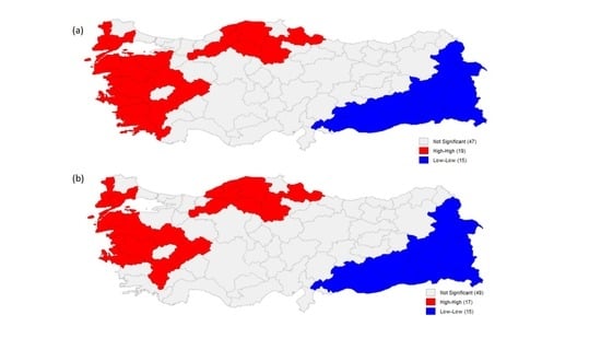
67] to detect the location of spatial clusters. The cluster maps for the dependent variable for 2012 and 2019 are presented in
Figure 4. According to the LISA results, it is clear that the high level of well-being is clustered in the western and northern parts of the country, whereas a low level of well-being is highly clustered in the eastern regions.
In order to benefit from controlling both spatial and time-specific effects [
66], we employ spatial panel models and explore spatial spillover effects. Recently, spatial panel models have been attracting a lot of attraction from researchers, but it is necessary to perform several preliminary specification procedures in order to select the best model [
68]. To choose a model, first, we ran the spatial Hausman test, and the results indicated that the fixed-effects model is appropriate (
Table 5). Afterwards, we used the LM tests and the robust LM tests for spatial error and spatial lag dependence in order to decide which model specification to employ. Both LM tests for lag and error dependence are significant, which provide evidence of spatial dependence in the data. To decide what type of spatial dependence will work, we looked at the robust LM test results, as indicated in [
69]. According to the robust LM test, the SAR has a lower
p-value, and thus the spatial lag fixed effects model performs better, which is also consistent with the previous spatial models in the literature. In Model 4, we ran fixed effects with all contagious variables while excluding dummies.
Table 5 presents the results from the spatial lag fixed-effects model. The spatial autocorrelation coefficient (λ), which is the coefficient parameter of the spatial lag term of the dependent variable, is added to the model. The spatial autocorrelation coefficient (λ) is highly significant and positive, which indicates spatial spillover effects. The spatial model results show that employment, schooling ratio, health problems, and density all have statistically significant effects, whereas GDP per capita has an insignificant impact on well-being. These results mean that the explanatory variable in a particular region affects the well-being of that particular region, as well as the well-being of neighbouring regions. Unlike aspatial models and spatial error models, for the SAR, it is necessary to calculate the direct effects (on the particular region) and the indirect effects (on the neighbouring regions) of the explanatory variables on the outcome. Following LeSage et al. [
70], we measure the direct and the indirect effects of the explanatory variables which are shown in the last three columns of
Table 5. According to the results, it is possible to state that the spillover effects of employment, health, density, and education variables are highly significant and lower than the direct effects.
7. Conclusions
Several subnational studies on well-being demonstrate that well-being is not evenly distributed over space, and spatial clusters of high and low well-being are evident. This study investigates the geography of regional well-being with a spatial emphasis on Turkish NUTS 3 regions, characterized by different environmental and urbanisation conditions. In order to understand the structure and pattern of well-being, we analysed the relationship between urbanism and well-being by considering city size, density, and urban–rural typology. We use 81 NUTS 3 regions and the time period 2012–2019 to analyse the geography of well-being for Turkey with panel and spatial panel models. According to the results, living in an urban area, in general, makes people happy, but population density negatively affects well-being. Analysis of the determinants of well-being reveals that education, health, employment, and income are all affecting well-being not only in the region itself but also in neighbouring regions as well. Our results indicate that ignoring spatial effects causes a misinterpretation of the effects of critical determinants of well-being in geography. As one of the primary goals of socio-economic development, enhancing well-being is on the agenda not only of researchers but also of policymakers. Therefore, it is crucial to measure, compare, and evaluate regional well-being periodically in order to gain a better understanding of the spatial pattern of well-being and its determinants and implement efficient, suitable policies for regions. Future studies might investigate the evaluation of the well-being of regions from a broader time span by considering their own characteristics of the regions, such as spatial and environmental, particularly.


