Abstract
To effectively reduce the impact of vegetation cover on surface settlement monitoring, the relationship between normalized difference vegetation index (NDVI) and coherence coefficient was established. It provides a way to estimate coherence coefficient by NDVI. In the research, a new method is tried to make the time range coincident between NDVI results and coherence coefficient results. Using the coherence coefficient results and the NDVI results of each interference image pair in the study area, the mathematical relationship between NDVI and the coherent coefficient was established based on statistical analysis of the fitting results of the exponential model, logarithmic model, and linear model. Four indicators were selected to evaluate the fitting results, including root mean square error, determinant coefficient, prediction interval coverage probability, and prediction interval normalized average width. The fitting effect of the exponential model was better than that of the logarithmic model and linear model. The mean of error was −0.041 in study area ROI1 and −0.126 in study area ROI2.The standard deviation of error was 0.165 in study area ROI1 and 0.140 in study area ROI2. The fitting results are consistent with the coherence coefficient results. The research method used the NDVI results to estimate the InSAR coherence coefficient. This provides an easy and efficient way to indirectly evaluate the interferometric coherence and a basis in InSAR data processing. The results can provide pre-estimation of coherence information in Ningxia by optical images.
1. Introduction
Interferometric synthetic aperture radar (InSAR) is a useful technique in generating a digital elevation model and monitoring surface deformation [1,2,3,4]. It is based on the phase difference of the echoes received by a satellite or aircraft. It has the advantage of acquiring data over a site during day or night time under all weather conditions and not impeded by cloud cover.
Interferometric coherence is one of the most important parameters for measuring the quality of interferograms in data processing of InSAR. It is predominantly evaluated using the coherence coefficient. The main factors affecting the interferometric coherence are Doppler decorrelation, thermal noise decorrelation, spatial decorrelation, and temporal decorrelation. Doppler decorrelation refers to a decorrelation phenomenon due to the inconsistency of the Doppler center frequency for twice imaging, which can be suppressed by azimuth filtering and can be further reduced by estimating the Doppler function [5]. The thermal noise decorrelation generates in the radar system when transmitting, receiving electromagnetic wave signals, and recording ground echo information [2]. Radar systems mainly rely on hardware settings to reduce the impact of system thermal noise. Spatial decorrelation refers to a decorrelation phenomenon caused by the spatial baseline of two radar images being too long and the side looking angles observed on the same targets for two images being different, resulting in considerable changes in phase [6]. The critical baseline can be used to evaluate the spatial decorrelation. With the baseline increasing, the correlation decreases. When the baseline increases to critical baseline, the coherence coefficient is 0. To reduce the effect of spatial decorrelation, it is necessary to set a short spatial baseline. Temporal decorrelation refers to a decorrelation phenomenon caused by large changes in the scattering characteristics of the ground objects when imaging twice [2]. To reduce the effect of temporal decorrelation, it is necessary to set a short temporal baseline. Additionally, long wavelength has a good effect on temporal correlation [7].
The growth of surface vegetation is one of the main factors causing the decorrelation of radar images. It is difficult to reduce its impact through post-processing. The normalized difference vegetation index (NDVI) can be obtained through calculations based on optical imagery and it is often used to monitor vegetation cover and growth. The relationship between NDVI and the coherence coefficient of radar images can effectively reflect the influence of vegetation cover on the interferometric coherence. There has been research conducted on it [8,9,10,11,12,13,14,15]. Bai et al. (2020) built a liner relationship between interferometric coherence and NDVI and found that the months with low NDVI are suitable for deformation monitoring [10]. Chen et al. (2021) used Landsat and ALOS-1 data to establish the relationship between NDVI and coherence coefficient in Meitanba in Hunan Province [14]. Liu et al. (2021) studied the relationship between the coherence coefficient and NDVI in southern China using linear and power function models and determined that it has a negative correlation relationship, considering the accuracy of the power function model is higher than that of the linear function model [15]. The relationship can be used in simple estimating of coherence coefficient.
The function between NDVI and coherence coefficient can be effectively used to extract the decoherent area covered by vegetation in the radar image with accessible optical images. It may provide an easy way to get the decoherent area in SAR images and provide a basis in InSAR data processing. In this study, we got the Sentinel-1 and Sentinel-2 images acquired in Ningxia Hui Autonomous Region, China. We established three models to establish the relationship between NDVI and the coherent coefficient and selected four indicators to evaluate the fitting results. The results can provide pre-estimation of coherence information in Ningxia by optical images.
This paper is organized as follows. In the next section, the study area and the data information of Sentinel-1 and Sentinel-2 are described in detail. The critical method for establishing the model is introduced in Section 3. A new method is tried to make the time range of NDVI results and coherence coefficient results coincident. Section 4 is dedicated to the presentation of the obtained results. Finally, conclusions are addressed.
2. Overview of the Study Area and Data
2.1. Overview of the Study Area
Located in the eastern part of Ningxia, the study area is in Yanchi County and is represented by red rectangles in Figure 1. ROI1 is used for model building and model accuracy validation. ROI2 is used for model feasibility analysis. The study area has a mid-temperate semi-arid continental monsoon climate. The climate is dry and hot, and the winter is severely cold and the summer is extremely hot with changeable conditions [16]. There are high diurnal fluctuations in temperature and the average annual temperature is approximately 9 °C, with the average annual precipitation being 205.2 mm [16]. The terrain of the study area is high in the south and low in the north, with a gentle terrain in the north.
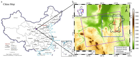
Figure 1.
(a) is China map and (b) is the location of the study area and remote sensing image coverage. Two red angles represent the study areas. A purple rectangle represents Sentinel-1 image coverage. A blue rectangle represents Sentinel-2 image coverage. And basemap bases on SRTM 30 m digital elevation model (DEM) data. Note: Figure (a) is based on the standard map with the review number GS(2019) 1673 downloaded from the standard map service website of the National Administration of Surveying, Mapping and Geographic Information, and the basemap has not been modified.
2.2. Data
2.2.1. Radar Data
Sentinel-l is a C-band radar satellite with a wavelength of approximately 5.6 cm, which has advantages of all-weather and day-and-night observation, a stable revisit time, and convenient access. Sentinel-1 has a 12-day revisit cycle and can be downloaded from the Earth Data website (https://asf.alaska.edu/ (accessed on 6 December 2021)). The time range of SAR images is from September 2017 to August 2018. The information of acquisition date is shown in Table A1. During the time range, study area ROI1 was stable without obvious deformation. It can reduce the impact of deformation on the model. Single look complex images were used in the research. The data scan mode is IW mode, with an ascending track mode. The Sentinel-1 image coverage is represented by a purple rectangle in Figure 1.
2.2.2. Optical Image Data
Sentinel-2 is a high-resolution multispectral imaging satellite, which consists of two satellites, Sentinel-2A and Sentinel-2B. Under cloudless conditions, the single-satellite revisit cycle is 10 days and the double-satellite revisit cycle can reach 5 days. Sentinel-2 has 12 bands and three resolutions, with detailed information shown in Table 1. The red band and the near-infrared band are used for NDVI calculation, and the resolution is 10 m. The Sentinel-2 image coverage is represented by a blue rectangle in Figure 1. The Sentinel-2 data includes two product levels: the L1C product and the L2A product. The L2A product can be obtained using the L1C product and atmospheric correction processing. The L2A product was used in the research and the cloud coverage was less than 10%. The information of optical image data used in the research is shown in Table A2.

Table 1.
Band information of Sentinel-2.
3. Modeling Processing
3.1. Preprocessing
Critical steps in preprocessing include obtaining the coherence coefficient of the radar images and the NDVI from optical images of the study area, resampling the NDVI results, selecting images, and using the maximum value composite (MVC) algorithm to calculate the NDVI.
3.1.1. Coherence Coefficient Calculation
Interferometric coherence is one of the key parameters for measuring the quality of interferograms in the data processing of InSAR and is mainly evaluated using the coherence coefficient. The coherence coefficient value is between . The higher the value, the better the interferometric coherence. The coherence coefficient calculation equation is shown in (1) [17,18].
where and represents the reference and secondary images, represents the conjugate complex number. The tool to calculate coherence coefficient is GMTSAR, an open source InSAR processing system [5,19], and the spatial resolution of the coherence coefficient results is 25 m. The DEM data is SRTM 30 m digital elevation model (DEM) data.
The information about interferometric pairs is shown in Table A3, and the coherence coefficient results are shown in Figure A1. The temporal baseline threshold for the interferometric images was 24 days, and the vertical baseline threshold was 100 m. A short perpendicular baseline means the high baseline correlation, which represents the high spatial correlation [20]. The equation for calculating baseline correlation is shown in (2) [21].
where represents perpendicular baseline and represents critical perpendicular baseline. The equation for calculating critical baseline is shown in (3) [21].
where is the wavelength, is the slant range, is the incident angle, is the slope, is the range resolution. Set Sentinel-1 as an example. is 90 km, is 44 degrees. We can get the critical perpendicular baseline is about 5 km by using (3) in the flat range. When the perpendicular baseline is 100 m, baseline correlation is about 0.98.
3.1.2. NDVI Calculation
The NDVI value is between [−1,1] and a negative value indicates that the surface is covered with water, ice, or snow. Zero indicates bare soil, rock, or buildings. Positive values indicate the presence of vegetation, and the NDVI value increases as vegetation cover increases. The NDVI calculation equation is shown in (4) and the NDVI results are shown in Figure A2.
where is the reflectance value of the near-infrared band and is the reflectivity value of the red band. The tool to calculate NDVI is SNAP, an open-source data processing software provided by the European Space Agency (ESA).
3.1.3. Resampling, Selecting Images, and Calculating the NDVI Using the MVC Algorithm
The resolution of the coherent coefficient images is equal to interferometric images. Because it is lower than the resolution of the NDVI images, the resolution of the NDVI images are resampled to the resolution of the coherent coefficient images so that there are same numbers of grids in the coherent coefficient and NDVI images.
In ideal conditions, the SAR data have a 12-day revisit cycle, and optical data have a 5-day revisit cycle. The imaging time being inconsistent between the NDVI, and the interferometric pairs is the main problem. Chen et al. (2021) solved this problem by establishing the relationship between the time baselines and the coherence coefficient, and introducing the time variable into the function of the NDVI and the coherence coefficient [14]. Liu et al. (2021) solved the inconsistency imaging problem between the NDVI and the interferometric pair based on the monthly NDVI dataset from 2016–2017 and by using the average coherence coefficient of the interferometric pairs for the months [15]. In this research, the MVC algorithm was used to calculate the NDVI images in the time range between the imaging time of the main and auxiliary images, so that the interferometric pair can correspond with the NDVI image. MVC refers to obtaining the maximum value of each grid in the NDVI images over a certain period, which is relatively easy to achieve. It can effectively reduce the influence of cloud, atmosphere, solar altitude angle, and other factors on remote sensing images and is widely used in the production of NDVI. The MVC results are shown in Figure A3.
3.2. Data Sampling
The images are sampled according to main parameter: the sample window size is pixels. Although the NDVI images were processed using the MVC method, there is a considerable number of grids containing information from the cloud, with water also having a considerable influence on the experiment. Because compared with the images of coherence coefficient and the NDVI in water, some values of the coherence coefficient and the NDVI are smaller than 0.2, so the grid need be masked. The mean value and the correlation coefficients R are calculated for sampling and selecting. If the correlation coefficient was greater than 0.6, the mean value of the coherence coefficient and the NDVI are fitted. The correlation coefficient calculation formula is shown in (5).
where and represent the value of each raster element, and and represent the mean value of the raster element being sampled.
3.3. Data Fitting Results Evaluation
The fitting functions are evaluated using the root mean square error (RMSE) and determined coefficient (). Under the condition of a 99% confidence level, the prediction intervals coverage probability (PICP) and the prediction intervals normalized averaged width (PINAW) are used to evaluate the fitting functions.
is the deviation between the true value and the predicted value, which is calculated as shown in (6). The smaller the RMSE value, the smaller the gap between the true and predicted values.
where is the true value and is the predictive value calculated by fitting function.
is used to determine the fitting degree of the regression equation, which is calculated as shown in (7). The value field is [0,1]. The larger the value, the better the degree of the model fitting.
where is the predictive value calculated by fitting function, is the true value, and is the average value.
The relationship among the three is:
where is the total square sum, is the residual square sum, and is the explained square sum.
PICP represents the actual frequency that observations fall within the prediction interval and is used to evaluate the reliability of the prediction interval, which is calculated as shown in (12) [22]. The higher the PICP value, the better the prediction result and the more reliable the model.
where is the sample size, is a Boolean variable that represents the relationship between the prediction interval and the observed value, is the sample truth value, and and are the smallest and biggest bounds of the prediction interval, respectively.
The formula for calculating the is shown in (13). A smaller value means a more sensitive prediction interval and more reliable model [22].
where is the sample size, is the range of the sample target variable, and and represent the smallest and biggest bounds of the prediction interval, respectively.
3.4. The Method of Model Accuracy Validation
Comparing the calculated coherence coefficient with the real coherence coefficient, the error can be obtained to evaluate the precision of the fitting function. The error calculation equation is shown in (14):
where represents the true coherence coefficient, and represents the predicted coherence coefficient calculated by and the NDVI image.
4. Results and Discussion
4.1. Data Fitting Results
The results from sampling are shown in Figure 2a. The range of the NDVI is and the range of the coherence coefficient is . The NDVI and the coherence coefficient show a negative relationship. With the increase in NDVI, the interferometric coherence decreases. The exponential model, linear model, and logarithmic model are used to fit and the fitting results are shown in (15), (16), and (17), and four evaluation indicators in Section 3.3 are used to evaluate the fitting functions.
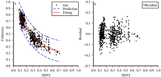
Figure 2.
Fitting result of exponential model (a) is the fitted curve graph, the red line is the fitted function curve, and the blue break line is the prediction interval curve. (b) is the residual graph.
As shown in Figure 2a, almost all the points are inside the prediction interval. Figure 2b is a residual distribution map, showing that that the residuals are roughly distributed and the residual distribution is relatively uniform. According to the statistical results, is 0.06272 and is 0.8767. Under the condition of a 99% confidence level, is 99.52% and is 0.3249.
As shown in Figure 3a, almost all the points are inside the prediction interval. Figure 3b is a residual distribution plot, showing that the residuals are roughly distributed [−0.3,0.3] and there is an anomaly in the residuals, which becomes larger when the NDVI value is higher than 0.6. According to the statistical results, is 0.07551 and is 0.8207. Under the condition of a 99% confidence level, is 99.36% and is 0.3908.
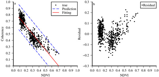
Figure 3.
Fitting result of linear model (a) is the fitted curve graph, the red line is the fitted function curve, and the blue break line is the prediction interval curve. (b) is the residual graph.
As shown in Figure 4a, almost all the points are inside the prediction interval. Figure 4b is a residual distribution plot, showing that the residuals are roughly distributed [−0.2,0.2] and the residual distribution is relatively uniform. According to the statistical results, is 0.06407 and is 0.8711. Under the condition of a 99% confidence level, is 99.36% and is 0.3316.
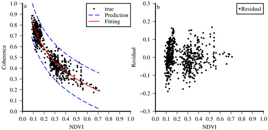
Figure 4.
Fitting result of logarithmic model (a) is the fitted curve graph, the red line is the fitted function curve, and the blue break line is the prediction interval curve. (b) is the residual graph.
The results of the evaluation are shown in Table 2. Comparing the , it can be considered that the gap between the true value and the predicted value of is less those of than and . Comparing , it can be seen that the model fits of is better than those of and . Under the condition of a 99% confidence level, comparing and , it can be seen that model reliability and prediction interval sensitivity of is higher than those of the others. In summary, the evaluation results are better than and . Therefore, it is more reliable to choose as the fitting function.
Table 2.
Evaluation results.
4.2. Model Accuracy Validation
One of interferometric pairs is selected to verify the precision of the fitting function in ROI1. The reference imaging time is 15 August 2019, and the secondary imaging time is 27 August 2019. The results are shown in Figure 5. Figure 5a shows the ROI1 NDVI result in the study area. Figure 5b shows the ROI1 coherence coefficient result in the study area. Figure 5c shows the error between the true values and the prediction values of the coherence coefficient. The overall fitting effect of the study area is good, and the larger error values are concentrated in the south of the study area. Figure 5d represents the error distribution, and the error is approximately followed by a normal distribution. The mean of error is −0.041, and the standard deviation of error is 0.165, with the error mainly being concentrated . Figure 5e is the slope distribution in ROI1.
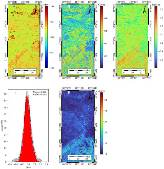
Figure 5.
Fit function accuracy verification plot of interferometric pair 20190815–20190827 in ROI1, (a) is the NDVI result; (b) is the coherence coefficient map; (c) is the error result; (d) is the error distribution; (e) is the slope of ROI1.
It can be seen from Figure 5c that the error in the northern part of the study area is . However, the estimated values in some areas are higher than the true values. In the southern part of the study area, there are larger error values. The estimated values for this area are predominantly lower than the true values. From Figure 5c,e, the large error values and high slope degrees have roughly the same spatial distribution. The high relief maybe the main reason for larger error values [14].
Then, another interferometric pair is selected, which has a temporal baseline of 24 days. The reference imaging time is 3 August 2019, and the secondary imaging time is 27 August 2019. The results are shown in Figure 6. Figure 6a shows the ROI1 NDVI result in the study area. Figure 6b shows the ROI1 coherence coefficient result in the study area. Figure 6c shows the error between the true values and the prediction values of the coherence coefficient. The overall fitting effect of the study area is good, and the larger error values are concentrated in the south of the study area. Figure 6d represents the error distribution and the error is approximately followed by a normal distribution. The mean of error is −0.069, and the standard deviation of error is 0.170, with the error mainly being concentrated . Figure 6e is the slope distribution in ROI1. The results shown in Figure 6 are consistent with the results shown in Figure 5. The mean and standard deviation of error show a small increase, and the large error values and high slope degrees show the same spatial distribution as Figure 5.
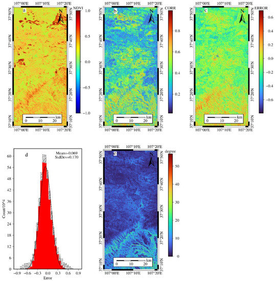
Figure 6.
Fit function accuracy verification plot of interferometric pair 20190803–20190827 in ROI1, (a) is the NDVI result; (b) is the coherence coefficient map; (c) is the error result; (d) is the error distribution; (e) is the slope of ROI1.
The other study area, ROI2, is used to verify model feasibility. The results are shown in Figure 7. Figure 7a shows the NDVI result of ROI2 and Figure 7b shows the prediction result of coherence coefficient in ROI2 by Figure 7a and fitting model. Figure 7c shows the true value of coherence coefficient in ROI2. Figure 7d shows the error between the true values and the prediction values of the coherence coefficient, and the overall fitting effect of the study area is good. Figure 7e shows the error distribution, and the error is approximately followed by the normal distribution. The mean of error is −0.126, and the standard deviation of error is 0.140, with the error being mainly concentrated . Figure 7f is the map of DEM, and Figure 7g is the map of slope. Figure 7h is the map of land use type distribution in 2018.
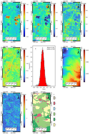
Figure 7.
Fit function accuracy verification plot of interferometric pair 20190803–20190827 in ROI2, (a) is the NDVI result; (b) is the prediction result of coherence coefficient; (c) is the coherence coefficient map; (d) is the error result; (e) is the error distribution; (f) is the map of DEM; (g) is the map of slope; (h) is the map of land use type distribution in 2018 [23], and T represents the land use type. Among them, 1 represents cultivated land, 2 represents woodland, 3 represents grassland, 4 represents waters, 5 represents urban and rural, industrial and mining, and residential land, construction land, and 6 represents unused land. Note: (f) is provided by Data Center for Resources and Environmental Sciences, Chinese Academy of Sciences (RESDC) (http://www.resdc.cn(accessed on 20 July 2021)).
Compared with Figure 7c, the prediction result of coherence coefficient in Figure 7b is consistent. The high NDVI value region in Figure 7a is the region with low coherence coefficient in Figure 7b,c. It can be seen from Figure 7d that the error is [−0.3,0.3], which is similar to the result showed in Figure 7e. Compared with the same interferometric pair result in ROI1, the absolute value of the mean error became larger and the standard deviation became smaller, with both following the normal distribution. Figure 7f,g shows ROI2 is flat area, and it is inconsistent between error distribution and slope degree. Figure 7d,h show that the larger error area distribution is generally in areas of urban and rural, industrial and mining and residential land, construction land, which are mostly misestimated. However, the results from ROI2 show that fits well for most of the area. Therefore, the model is effective.
In this paper, an empirical model for NDVI and the coherence coefficient is obtained for study area ROI1 and the model accuracy is verified in study areas ROI1 and ROI2. Research shows that the model is reliable. The research result is useful in DInSAR data processing of deformation monitoring:
(1) The NDVI value can be used as a standard for evaluating the usability in DInSAR. It would be good with lower NDVI and bad in higher NDVI area. It is not useful in area when NDVI higher than 0.4. In this condition, longer band SAR data or technology is better.
(2) It can be used to reduce the impact of vegetation in deformation monitor. The deformation got in DInSAR technology should be masked in higher NDVI to improve the deformation result reliable.
(3) It also can used as a basis to evaluate the precision of InSAR monitoring results. The DInSAR deformation results and precision with different NDVI area should be discussed separately. It is an important basis to calculate the error of DInSAR deformation results.
In the future, the different types of land cover in the correlation between NDVI and interferometric coherence should be considered [24]. Also, introducing a time parameter to the model maybe a good idea [14]. In addition, the model connected among multi-band, multi-polarization, and multi-vegetation indexes can be built [9].
5. Conclusions
The relationship between NDVI and interferometric coherence in Ningxia was studied using optical images and C-band SAR images and an empirical model between the NDVI and the coherence coefficient was constructed through fitting analysis. The main conclusions were as follows:
(1) In the research, a new way is used to make the time range of NDVI results and coherence coefficient results coincident. The good fitting results show that it may be a good way to study the relationship between NDVI and interferometric coherence.
(2) Three statistical models between the coherence coefficient and the NDVI were constructed using the exponential model, logarithmic model, and linear model. The RMSE, determinant coefficient, PICP, and PINAW, under the condition of a 99% confidence level, are calculated, respectively. Results show that the fitting effect of the exponential model is better than the other models. Based on the exponential function, the calculation accuracy was analyzed in study areas ROI1 and ROI2. Results showed that the error of the calculation conformed to the normal distribution. The mean of error was −0.041 in ROI1 and −0.126 in ROI2. The standard deviation of error was 0.165 in ROI1 and 0.140 in ROI2, which showed good fitting results using the exponential function.
(3) The result shows that it is possible to evaluate the coherence coefficient values using optical remote sensing data. It can be the complementary content to the study of the relationship between NDVI and coherence and can guide the selection of incoherent areas in radar images due to excessive vegetation coverage, which can provide the basis for DInSAR data processing of deformation monitoring. The results can provide pre-estimation of coherence information in Ningxia by optical images.
Author Contributions
Methodology, Y.C.; software, D.H.; resources, Y.L. and S.Z.; writing—original draft, Y.C.; writing—review & editing, P.L. and Y.W.; project administration, P.L.; funding acquisition, P.L. All authors have read and agreed to the published version of the manuscript.
Funding
This study was funded by the Fundamental Research Funds for the Central Universities (Grant Nos. 2022YQDC01 and 2022YJSDC08), the Ecological-Smart Mines Joint Research Fund of the Natural Science Foundation of Hebei Province (Grant No. E2020402086), and open funds from the State Key Laboratory of Coal Mining and Clean Utilization (Granted No.2021-CMCU-KF014).
Institutional Review Board Statement
Not applicable.
Informed Consent Statement
Not applicable.
Data Availability Statement
Not applicable.
Acknowledgments
The authors would like to acknowledge the open datasets of Sentinel-1 and Sentinel-2 and the data processing soft SNAP provided by the European Space Agency (ESA). The authors would like to acknowledge an InSAR processing system GMTSAR based on GMT.
Conflicts of Interest
The authors declare no conflict of interest.
Appendix A
Table A1.
Sentinel-1 acquisition date information.
Table A1.
Sentinel-1 acquisition date information.
| Num | Imaging Time | Num | Imaging Time | Num | Imaging Time |
|---|---|---|---|---|---|
| 1 | 20180901 | 12 | 20190111 | 22 | 20190511 |
| 2 | 20180913 | 13 | 20190123 | 23 | 20190523 |
| 3 | 20180925 | 14 | 20190204 | 24 | 20190604 |
| 4 | 20181007 | 15 | 20190216 | 25 | 20190616 |
| 5 | 20181019 | 16 | 20190228 | 26 | 20190628 |
| 6 | 20181031 | 17 | 20190312 | 27 | 20190710 |
| 7 | 20181112 | 18 | 20190324 | 28 | 20190722 |
| 8 | 20181124 | 19 | 20190405 | 29 | 20190803 |
| 9 | 20181206 | 20 | 20190417 | 30 | 20190815 |
| 10 | 20181218 | 21 | 20190429 | 31 | 20190827 |
| 11 | 20181230 |
Table A2.
Sentinel-2 acquisition date information.
Table A2.
Sentinel-2 acquisition date information.
| Num | Imaging Time | Num | Imaging Time | Num | Imaging Time |
|---|---|---|---|---|---|
| 1 | 20181218 | 7 | 20190318 | 13 | 20190522 |
| 2 | 20190102 | 8 | 20190323 | 14 | 20190601 |
| 3 | 20190107 | 9 | 20190328 | 15 | 20190606 |
| 4 | 20190117 | 10 | 20190417 | 16 | 20190706 |
| 5 | 20190122 | 11 | 20190512 | 17 | 20190731 |
| 6 | 20190211 | 12 | 20190517 | 18 | 20190815 |
Table A3.
Interferometric information.
Table A3.
Interferometric information.
| Num | Reference Image | Secondary Image | Temporal Baseline /m | Perpendicular Baseline /m | Resolution /m |
|---|---|---|---|---|---|
| 1 | 20180901 | 20180913 | 12 | 87.0489 | 25 |
| 2 | 20180913 | 20180925 | 12 | 36.5774 | 25 |
| 3 | 20180913 | 20181007 | 24 | 27.866 | 25 |
| 4 | 20180925 | 20181007 | 12 | 8.71134 | 25 |
| 5 | 20181007 | 20181019 | 12 | 96.421 | 25 |
| 6 | 20181019 | 20181031 | 12 | 4.10631 | 25 |
| 7 | 20181019 | 20181112 | 24 | 54.6995 | 25 |
| 8 | 20181031 | 20181112 | 12 | 58.8058 | 25 |
| 9 | 20181112 | 20181124 | 12 | 78.5131 | 25 |
| 10 | 20181112 | 20181206 | 24 | 20.324 | 25 |
| 11 | 20181124 | 20181206 | 12 | 58.1891 | 25 |
| 12 | 20181124 | 20181218 | 24 | 9.97468 | 25 |
| 13 | 20181206 | 20181218 | 12 | 48.2144 | 25 |
| 14 | 20181206 | 20181230 | 24 | 39.6463 | 25 |
| 15 | 20181218 | 20181230 | 12 | 87.8607 | 25 |
| 16 | 20181218 | 20190111 | 24 | 66.7602 | 25 |
| 17 | 20181230 | 20190111 | 12 | 21.1005 | 25 |
| 18 | 20181230 | 20190123 | 24 | 10.6224 | 25 |
| 19 | 20190111 | 20190123 | 12 | 10.4781 | 25 |
| 20 | 20190123 | 20190216 | 24 | 40.7835 | 25 |
| 21 | 20190204 | 20190216 | 12 | 96.5544 | 25 |
| 22 | 20190216 | 20190228 | 12 | 74.7184 | 25 |
| 23 | 20190216 | 20190312 | 24 | 75.875 | 25 |
| 24 | 20190228 | 20190312 | 12 | 1.15659 | 25 |
| 25 | 20190228 | 20190324 | 24 | 8.94817 | 25 |
| 26 | 20190312 | 20190324 | 12 | 7.79159 | 25 |
| 27 | 20190312 | 20190405 | 24 | 36.0626 | 25 |
| 28 | 20190324 | 20190405 | 12 | 43.8542 | 25 |
| 29 | 20190324 | 20190417 | 24 | 44.4763 | 25 |
| 30 | 20190405 | 20190417 | 12 | 0.622107 | 25 |
| 31 | 20190405 | 20190429 | 24 | 96.1843 | 25 |
| 32 | 20190417 | 20190429 | 12 | 96.8064 | 25 |
| 33 | 20190417 | 20190511 | 24 | 23.9404 | 25 |
| 34 | 20190429 | 20190511 | 12 | 72.866 | 25 |
| 35 | 20190429 | 20190523 | 24 | 96.0215 | 25 |
| 36 | 20190511 | 20190523 | 12 | 23.1555 | 25 |
| 37 | 20190511 | 20190604 | 24 | 38.3302 | 25 |
| 38 | 20190523 | 20190604 | 12 | 15.1747 | 25 |
| 39 | 20190523 | 20190616 | 24 | 59.171 | 25 |
| 40 | 20190604 | 20190616 | 12 | 43.9963 | 25 |
| 41 | 20190604 | 20190628 | 24 | 30.9379 | 25 |
| 42 | 20190616 | 20190628 | 12 | 74.9343 | 25 |
| 43 | 20190616 | 20190710 | 24 | 56.8686 | 25 |
| 44 | 20190628 | 20190710 | 12 | 18.0656 | 25 |
| 45 | 20190628 | 20190722 | 24 | 32.9689 | 25 |
| 46 | 20190710 | 20190722 | 12 | 51.0345 | 25 |
| 47 | 20190710 | 20190803 | 24 | 32.2786 | 25 |
| 48 | 20190722 | 20190803 | 12 | 83.3131 | 25 |
| 49 | 20190722 | 20190815 | 24 | 56.3615 | 25 |
| 50 | 20190803 | 20190815 | 12 | 26.9516 | 25 |
| 51 | 20190803 | 20190827 | 24 | 68.1896 | 25 |
| 52 | 20190815 | 20190827 | 12 | 41.2379 | 25 |

Figure A1.
Result of γ.
Figure A1.
Result of γ.


Figure A2.
The result of NDVI.
Figure A2.
The result of NDVI.


Figure A3.
Result of MVC.
Figure A3.
Result of MVC.

References
- Rosenp, A.; Hensleys, S.; Joughin, I.R.; Li, F.K.; Madsen, S.N.; Rodriguez, E.; Goldstein, R.M. Synthetic aperture radar interferometry. Proc. IEEE 2000, 88, 333–382. [Google Scholar] [CrossRef]
- Moreira, A.; Prats-Iraola, P.; Younis, M.; Krieger, G.; Hajnsek, I.; Papathanassiou, K.P. A Tutorial on Synthetic Aperture Radar. IEEE Geosci. Remote Sens. Mag. 2013, 1, 6–43. [Google Scholar] [CrossRef]
- Yufen, N.I.U. Applications of SAR interferometry for co-seismic, interseismic and volcano deformation monitoring, modeling and interpretation. Acta Geod. Cartogr. Sin. 2022, 51, 471. [Google Scholar]
- Meng, Z.; Shu, C.; Yang, Y.; Wu, C.; Dong, X.; Wang, D.; Zhang, Y. Time Series Surface Deformation of Changbaishan Volcano Based on Sentinel-1B SAR Data and Its Geological Significance. Remote Sens. 2022, 14, 1213. [Google Scholar] [CrossRef]
- Sandwell, D.; Mellors, R.; Tong, X.; Wei, M.; Wessel, P. GMTSAR: An InSAR Processing System Based on Generic Mapping Tools: LLNL-TR-481284, 1090004[R/OL]. 2016: LLNL-TR-481284, 1090004[2022-09-02]. Available online: https://www.osti.gov/servlets/purl/1090004/ (accessed on 1 June 2022).
- Zebker, H.A.; Villasenor, J. Decorrelation in interferometric radar echoes. IEEE Trans. Geosci. Remote Sens. 1992, 30, 950–959. [Google Scholar] [CrossRef]
- Massonnet, D.; Feigl, K.L. Radar interferometry and its application to changes in the Earth’s surface. Rev. Geophys. 1998, 36, 441–500. [Google Scholar] [CrossRef]
- Arab-Sedze, M.; Heggy, E.; Bretar, F.; Berveiller, D.; Jacquemoud, S. Quantification of L-band InSAR coherence over volcanic areas using LiDAR and in situ measurements. Remote Sens. Environ. 2014, 152, 202–216. [Google Scholar] [CrossRef]
- Wang, C.; Fan, J.; Lin, S.; Rao, Y.; Huang, H. Study of the correlation between optical vegetation index and SAR data and the main affecting factors. Remote Sens. Land Resour. 2020, 32, 130–137. [Google Scholar]
- Bai, Z.; Fang, S.; Gao, J.; Zhang, Y.; Jin, G.; Wang, S.; Zhu, Y.; Xu, J. Could Vegetation Index be Derive from Synthetic Aperture Radar?—The Linear Relationship between Interferometric Coherence and NDVI. Sci. Rep. 2020, 10, 6749. [Google Scholar] [CrossRef] [PubMed]
- Liao, T.-H.; Simard, M.; Denbina, M.; Lamb, M.P. Monitoring Water Level Change and Seasonal Vegetation Change in the Coastal Wetlands of Louisiana Using L-Band Time-Series. Remote Sens. 2020, 12, 2351. [Google Scholar] [CrossRef]
- Pulella, A.; Aragão Santos, R.; Sica, F.; Posovszky, P.; Rizzoli, P. Multi-Temporal Sentinel-1 Backscatter and Coherence for Rainforest Mapping. Remote Sens. 2020, 12, 847. [Google Scholar] [CrossRef]
- Nikaein, T.; Iannini, L.; Molijn, R.A.; Lopez-Dekker, P. On the Value of Sentinel-1 InSAR Coherence Time-Series for Vegetation Classification. Remote Sens. 2021, 13, 3300. [Google Scholar] [CrossRef]
- Chen, Y.; Sun, Q.; Hu, J. Quantitatively Estimating of InSAR Decorrelation Based on Landsat-Derived NDVI. Remote Sens. 2021, 13, 2440. [Google Scholar] [CrossRef]
- Liu, Z.Y.; Zhang, C.; Liu, Z.K.; Yuan, J.J.; Qi, H.C.; Pan, Y.F.; Zhu, H.L.; Wu, X.W.; Wang, H. Empirical relationship between radar coherence and NDVI. Bull. Surv. Mapp. 2021, 4, 45–51+59. [Google Scholar] [CrossRef]
- Ningxia Provincial Bureau of Statistics; Nbs Survey of-Fice in Ningxia. Ning Xia Statistical Yearbook; China Statistics Press: Beijing, China, 2018. [Google Scholar]
- Bamler, R.; Hartl, P. Synthetic aperture radar interferometry. Inverse Problems 1998, 14, 1–54. [Google Scholar] [CrossRef]
- Touzi, R.; Lopes, A.; Bruniquel, J.; Vachon, P.W. Coherence estimation for S-AR imagery. IEEE Trans. Geosci. Remote Sens. 1999, 37, 15. [Google Scholar] [CrossRef]
- Sandwell, D.; Mellors, R.; Tong, X.; Wei, M.; Wessel, P. Open radar interferometry software for mapping surface Deformation. Eos Trans. Am. Geophys. Union 2011, 92, 234. [Google Scholar] [CrossRef]
- Wang, Z.; Tang, X.; Li, T. Impact Analysis of InSAR Spatio-temporal Baseline on DEM Accuracy. Bull. Surv. Mapp. 2018, 2, 61–66. [Google Scholar] [CrossRef]
- Liu, G.X.; Chen, Q.; Luo, X.J.; Cai, G.L. InSAR Principle and Application; Science Press: Beijing, China, 2019. [Google Scholar]
- Chen, X.; Lai, C.S.; Ng, W.W.Y.; Pan, K.; Lai, L.L.; Zhong, C. A stochastic sensitivity-based m-ulti-objective optimization method for short-term wind speed interval prediction. Int. J. Mach. Learn. Cybern. 2021, 12, 2579–2590. [Google Scholar] [CrossRef]
- Xu, X.; Liu, J.; Zhang, S.; Li, R.; Yan, C.; Wu, S. Remote Sensing Monitoring Dataset of Land Use and Land Cover in China over Multiple Periods(CNLUCC); Data Registration and Publication System, Institute of Geographic Sciences and Natural Resources Research, Chinese Academy of Sciences: Beijing, China, 2018. [Google Scholar] [CrossRef]
- Villarroya-Carpio, A.; Lopez-Sanchez, J.M.; Engdahl, M.E. Sentinel-1 interferometric coherence as a vegetation index for agriculture. Remote Sens. Environ. 2022, 280, 113208. [Google Scholar] [CrossRef]


Publisher’s Note: MDPI stays neutral with regard to jurisdictional claims in published maps and institutional affiliations. |
© 2022 by the authors. Licensee MDPI, Basel, Switzerland. This article is an open access article distributed under the terms and conditions of the Creative Commons Attribution (CC BY) license (https://creativecommons.org/licenses/by/4.0/).