


Identifying Causes of Traffic Crashes Associated with Driver Behavior Using Supervised Machine Learning Methods: Case of Highway 15 in Saudi Arabia

 ,
,  , , and
Abstract
:1. Introduction
2. Background and Literature Review
2.1. Causes of RTCs
2.2. Machine Learning (ML) Models in RTC Analyses
3. Materials and Methods
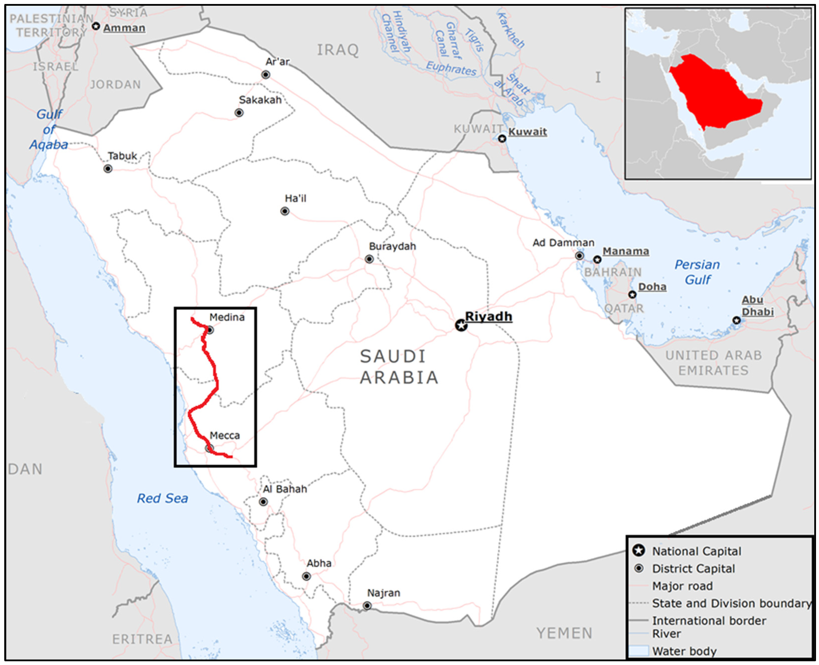
3.1. Study Site
3.2. Materials
Preprocessing Data
- Getting the data to know: This step studied the various attribute types, which included nominal, binary, ordinal, and numeric attributes. Basic descriptive statistics are used to learn more about each attribute’s values. Knowing basic statistics makes it easier to fill in missing values, smooth noisy values, and spot outliers in the data preprocessing stage. Knowing attributes and their values can also help deal with inconsistencies incurred during data integration. Visualization of the RTC data provided information on the trend of the main attributes used in modeling.
- Checking the completeness: This step was carried out by checking the completeness of the main attributes of crash occurrences, such as the crash type, road and weather conditions, number of casualties and injuries, crash reasons and remarks, and road geometry. Some missing data were imputed with information available from other attributes, but some could not. For example, 943 out of 3439 cases were missing “road geometry” attributes that could not be imputed and coded as ‘unknown’ or ‘other’ in the variables used to describe roadway geometry.
- Imputing missing data: Data with missing values for some attributes are quite common. There are various methods for handling the problem of missing values in data. Here, using the most probable value to fill in the missing value was preferred and determined with decision tree induction using non-missing crash attributes in the data set [46].
- Normalization: Data normalization gives all attributes an equal weight, where the values are scaled to a smaller range, such as 0.0 to 1.0. Normalization benefits classification algorithms such as neural networks or distance-based models. Normalizing the values for each attribute included in the training set helps speed up the learning phase when using the neural network backpropagation algorithm for classification. For distance-based methods, normalization prevents attributes with large ranges (e.g., AADT, min = 2083 and max = 60,244) from outweighing small-range attributes (e.g., binary variables). There are several methods used for normalization. The min-max normalization was selected in this study. Min-max normalization transforms a value x of a numeric variable V to in the range (0, 1), as shown in Equation (1) below.
3.3. Methods
3.3.1. Analysis of RTCs
3.3.2. Modeling of RTCs
4. Results and Discussion
4.1. Descriptive Statistics and Visualization of RTC Factors
4.2. Modeling Results
4.2.1. Results of BNLOGREG
4.2.2. Comparison of BNLOGREG with Machine-Learning Algorithms
4.2.3. Discussion of the Results and Research Limitations
4.3. Crash Prevention and Mitigation Strategies
4.3.1. Designing Safe Roads and Maintaining Work Zone Safety
4.3.2. Driver Education and Awareness
4.3.3. Application of Advance Technologies
4.3.4. In-Vehicle Technologies and Autonomous Driving
4.3.5. Legislation and Enforcement of Traffic Regulations
4.3.6. Benefits of Academic Studies and Research on Traffic Safety
5. Summary and Conclusions
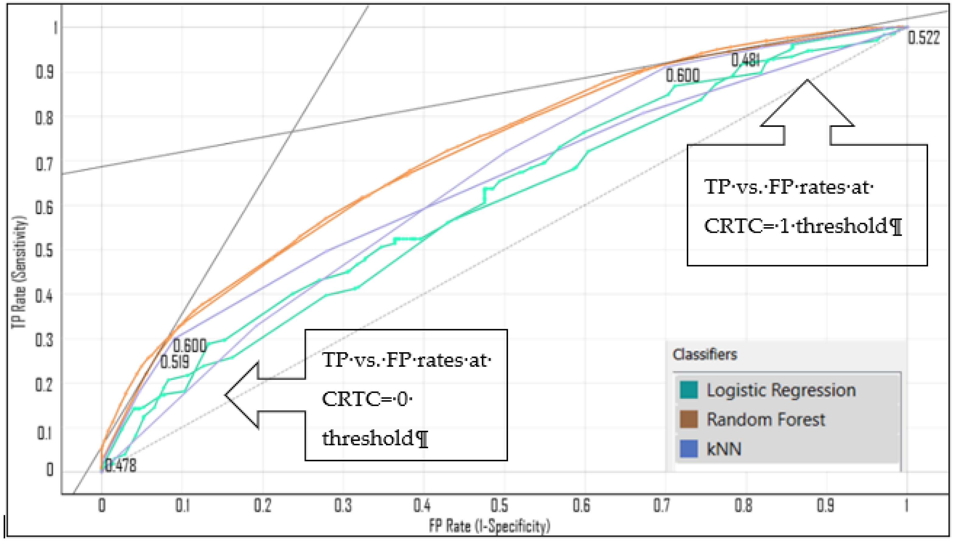
- The performance of all models is comparable, so they are found to be suitable for predicting the probability of driver errors in the occurrence of RTCs and understanding the role of the input variables in explaining the model outcomes.
- The two most influential variables are ASF and AADT in the RF model. In line with the findings of previous research conducted in a similar study context, an increase in the number of lanes (NL) and daily average speed of traffic flow (ASF) reduces the likelihood of the RTCs caused by driver errors. This finding is also supported by the results of previous studies [32,67]. In contrast, an increase in traffic volume (AADT) and the road geometry features (straight sections and horizontal curves) significantly contributed to driver errors leading to RTCs.
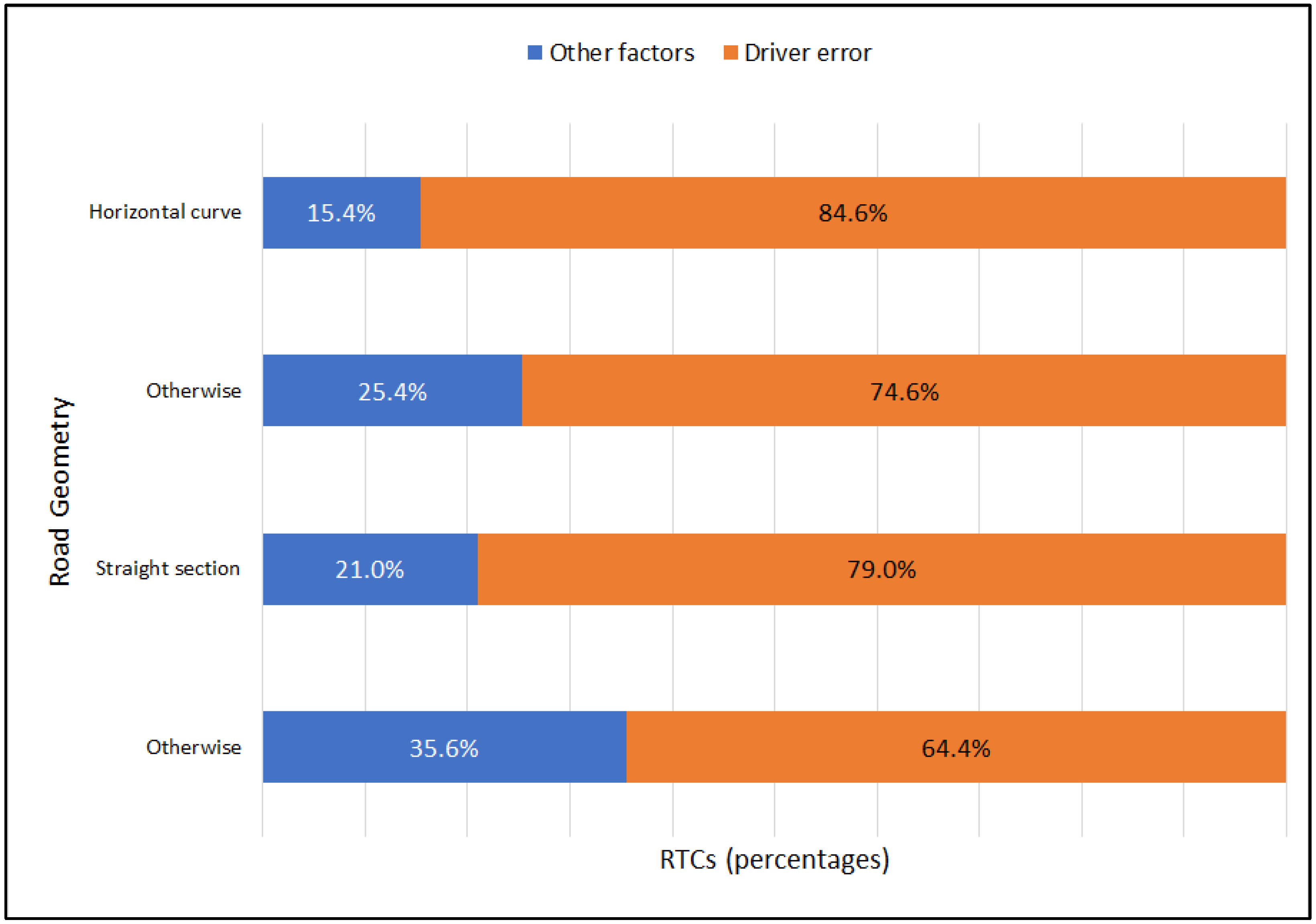
- Straight road sections and the sections with horizontal curves increase the probability of driver-error-related RTCs by more than two and three folds (odds ratios = 2.280 and 3.555 yielded by BNLOGREG).
- The inferences concerning the effects of crash attributes are in agreement with the findings in the literature. Thus, the paper sufficiently contributes to insufficient knowledge of the factors in RTCs on major roads within the context of this case study.
Author Contributions
Funding
Institutional Review Board Statement
Informed Consent Statement
Data Availability Statement
Acknowledgments
Conflicts of Interest
Appendix A
References
- Rahman, M.M.; Islam, M.K.; Al-Shayeb, A.; Arifuzzaman, M. Towards Sustainable Road Safety in Saudi Arabia: Exploring Traffic Accident Causes Associated with Driving Behavior Using a Bayesian Belief Network. Sustainability 2022, 14, 6315. [Google Scholar] [CrossRef]
- United Nations|Saudi Arabia: World Health Organization Together with the Ministry of Health and Ministry of Interior. Join Efforts to Reduce Mortality from Road Traffic Accidents. Available online: https://saudiarabia.un.org/en/105869-world-health-organization-together-ministry-health-and-ministry-interior-join-efforts-reduce (accessed on 9 September 2022).
- Transport and Infrastructure in Saudi Arabia. Available online: https://www.worlddata.info/asia/saudi-arabia/transport.php (accessed on 29 October 2022).
- Worldbank. Saudi Arabia|Overview. Available online: https://data.worldbank.org/country/SA (accessed on 7 October 2022).
- General Authority for Statistics (GSTAT), 2021. Population Estimates in the Midyear of 2021. Available online: https://www.stats.gov.sa/sites/default/files/POP%20SEM2021E.pdf (accessed on 27 August 2022).
- Alghnam, S.; Alkelya, M.; Alfraidy, M.; Al-Bedah, K.; Albabtain, I.T.; Alshenqeety, O. Outcomes of road traffic injuries before and after the implementation of a camera ticketing system: A retrospective study from a large trauma center in Saudi Arabia. Ann. Saudi Med. 2017, 37, 1–9. [Google Scholar] [CrossRef] [PubMed] [Green Version]
- Sauber-Schatz, E.K.; Parker, E.M.; Sleet, D.A.; Ballesteros, M.F. Road & Traffic Safety—Chapter 8—Yellow Book|Travelers’ Health|CDC, 2020. Available online: https://wwwnc.cdc.gov/travel/yellowbook/2020/travel-by-air-land-sea/road-and-traffic-safety (accessed on 7 October 2022).
- WISQARS (Web-based Injury Statistics Query and Reporting System)|Injury Center|CDC, 2021. Available online: https://www.cdc.gov/injury/wisqars/index.html (accessed on 7 October 2022).
- Ministry of Health Saudi Arabia (MOH). Available online: https://www.moh.gov.sa/en/Pages/Default.aspx (accessed on 28 October 2022).
- Harbeck, E.L.; Glendon, A.I.; Hine, T.J. Young driver perceived risk and risky driving: A theoretical approach to the “fatal five”. Transp. Res. Part F Traffic Psychol. Behav. 2018, 58, 392–404. [Google Scholar] [CrossRef]
- Shen, S.; Neyens, D.M. Factors affecting teen drivers’ crash-related length of stay in the hospital. J. Transp. Health 2016, 4, 162–170. [Google Scholar] [CrossRef]
- Shaaban, K.; Gaweesh, S.; Ahmed, M.M. Investigating in-vehicle distracting activities and crash risks for young drivers using structural equation modeling. PLoS ONE 2020, 15, e0235325. [Google Scholar] [CrossRef] [PubMed]
- Ansari, S.; Akhdar, F.; Mandoorah, M.; Moutaery, K. Causes and effects of road traffic accidents in Saudi Arabia. Public Health 2000, 114, 37–39. [Google Scholar] [CrossRef] [PubMed]
- Patterson, T.L.; Frith, W.J.; Small, M.W. Down with Speed: A Review of the Literature, and the Impact of Speed on New Zealanders; Accident Compensation Corporation and Land Transport Safety Authority: Wellington, New Zealand, 2000. [Google Scholar]
- Ladegaard, I. For Drivers with Heavy Eyelids, Good Roads can Kill, 2012. Available online: https://sciencenorway.no/cars-and-traffic-forskningno-norway/for-drivers-with-heavy-eyelids-good-roads-can-kill/1373723 (accessed on 11 August 2022).
- Hauer, E. Speed and safety. Transport. Res. Rec. 2009, 2103, 10–17. [Google Scholar] [CrossRef] [Green Version]
- Montella, A.; Imbriani, L.L. Safety performance functions incorporating design consistency variables. Accid. Anal. Prev. 2015, 74, 133–144. [Google Scholar] [CrossRef] [PubMed]
- Wang, C.; Quddus, M.A.; Ison, S.G. Predicting accident frequency at their severity levels and its application in site ranking using a two-stage mixed multivariate model. Accid. Anal. Prev. 2011, 43, 1979–1990. [Google Scholar] [CrossRef] [Green Version]
- Yau, K.K.W. Risk factors affecting the severity of single-vehicle traffic accidents in Hong Kong. Accid. Anal. Prev. 2004, 36, 333–340. [Google Scholar] [CrossRef] [PubMed]
- Yu, R.; Abdel-Aty, M. Analyzing crash injury severity for a mountainous freeway incorporating real-time traffic and weather data. Saf. Sci. 2014, 63, 50–56. [Google Scholar] [CrossRef]
- Montella, A.; Andreassen, D.; Tarko, A.; Turner, S.; Mauriello, F.; Imbriani, L.L.; Romero, M. Crash databases in Australasia, the European Union, and the United States: Review and prospects for improvement. Transport. Res. Rec. 2013, 2386, 128–136. [Google Scholar] [CrossRef]
- Montella, A.; Imbriani, L.L.; Marzano, V.; Mauriello, F. Effects on speed and safety of point-to-point speed enforcement systems: Evaluation on the urban motorway A56 Tangenziale di Napoli. Accid. Anal. Prev. 2015, 74, 133–144. [Google Scholar] [CrossRef] [PubMed]
- NHTSA. MMUCC Guideline: Model Minimum Uniform Crash Criteria—5th ed. Rep. DOT HS 2017, 812, 433. [Google Scholar]
- Viallon, V.; Laumon, B. Fractions of fatal crashes attributable to speeding: Evolution for the period 2001–2010 in France. Accid. Anal. Prev. 2013, 52, 250–256. [Google Scholar] [CrossRef]
- Ratanavaraha, V.; Suangka, S. Impacts of accident severity factors and loss values of crashes on expressways in Thailand. IATSS Res. 2014, 37, 130–136. [Google Scholar] [CrossRef] [Green Version]
- Aarts, L.; van Schagen, I. Driving speed and the risk of road crashes: A review. Accid. Anal. Prev. 2006, 38, 215–224. [Google Scholar] [CrossRef]
- Hummer, J.E.; Rasdorf, W.; Findley, D.J.; Zegeer, C.V.; Sundstrom, C.A. Procedure for Curve Warning Signing, Delineation, and Advisory Speeds for Horizontal Curves; NCDOT Report, No. FHWA/NC/2009-07; North Carolina Department of Transportation: Raleigh, NC, USA, 2010. [Google Scholar]
- Findley, D.J.; Hummer, J.E.; Rasdorf, W.; Zegeer, C.V.; Fowler, T.J. Modeling the impact of spatial relationships on horizontal curve safety. Accid. Anal. Prev. 2012, 45, 296–304. [Google Scholar] [CrossRef]
- Glennon, J.C. Effect of Alignment on Highway Safety. State of the Art Report 6; Transportation Research Board. National Research Council: Washington, DC, USA, 1987. [Google Scholar]
- Zegeer, C.V.; Stewart, J.R.; Council, F.M.; Reinfurt, D.W.; Hamilton, E. Safety Effects of Geometric Improvements on Horizontal Curves. Transport. Res. Rec. 1992, 1356, 11–19. [Google Scholar]
- Bauer, K.M.; Harwood, D.W. Safety Effects of Horizontal Curve and Grade Combinations on Rural Two-Lane Highways. Transport. Res. Rec. 2013, 2398, 37–49. [Google Scholar] [CrossRef] [Green Version]
- Garber, N.J.; Gadiraju, R. Factors affecting speed variance and its influence on accidents. Transport. Res. Rec. 1989, 1213, 64–71. [Google Scholar]
- Guido, G.; Shaffiee Haghshenas, S.; Vitale, A.; Astarita, V.; Park, Y.; Geem, Z.W. Evaluation of Contributing Factors Affecting Number of Vehicles Involved in Crashes Using Machine Learning Techniques in Rural Roads of Cosenza, Italy. Safety 2022, 8, 28. [Google Scholar] [CrossRef]
- Farhangi, F.; Sadeghi-Niaraki, A.; Razavi-Termeh, S.V.; Choi, S.-M. Evaluation of Tree-Based Machine Learning Algorithms for Accident Risk Mapping Caused by Driver Lack of Alertness at a National Scale. Sustainability 2021, 13, 10239. [Google Scholar] [CrossRef]
- Tamakloe, R.; Park, D. Factors Influencing Fatal Vehicle-Involved Crash Consequence Metrics at Spatio-Temporal Hotspots in South Korea: Application of GIS and Machine Learning Techniques. Int. J. Urban Sci. 2022, 1–35. [Google Scholar] [CrossRef]
- Tamakloe, R.; Sam, E.F.; Bencekri, M.; Das, S.; Park, D. Mining groups of factors influencing bus/minibus crash severities on poor pavement condition roads considering different lighting status. Traffic inj. Prev. 2022, 23, 308–314. [Google Scholar] [CrossRef]
- Mirzahossein, H.; Sashurpour, M.; Hosseinian, S.M.; Gilani, V.N.M. Presentation of machine learning methods to determine the most important factors affecting road traffic accidents on rural roads. Front. Struct. Civ. Eng. 2022, 16, 657–666. [Google Scholar] [CrossRef]
- Hu, P.; Li, Y.; Liu, Y.; Guo, G.; Gao, X.; Su, Z.; Wang, L.; Deng, G.; Yang, S.; Qi, Y.; et al. Comparison of Conventional Logistic Regression and Machine Learning Methods for Predicting Delayed Cerebral Ischemia After Aneurysmal Subarachnoid Hemorrhage: A Multicentric Observational Cohort Study. Front. Aging Neurosci. 2022, 14, 857521. [Google Scholar] [CrossRef]
- Han, J.; Kamber, M.; Pei, J. Data Mining: Concepts and Techniques, 3rd ed.; Morgan Kaufmann: Burlington, MA, USA, 2011; p. 391. [Google Scholar] [CrossRef]
- Glubb, J.B. Mecca|Definition, History, Pilgrimage, Population, Kaaba, City, & Facts|Britannica, 2022. Available online: https://www.britannica.com/place/Mecca (accessed on 7 October 2022).
- Glubb, J.B.; Abdo, A.S. Madinah|Britannica, 2022. Available online: https://www.britannica.com/place/Medina-Saudi-Arabia (accessed on 7 October 2022).
- Bujang, M.A.; Sa’at, N.; Joys, A.R.; Ali, M.M. An audit of the statistics and the comparison with the parameter in the population. In Proceedings of the AIP Conference Proceedings 1682, Selangor, Malaysia, 22 October 2015. [Google Scholar] [CrossRef]
- Bujang, M.A.; Ghani, P.A.; Bujang, M.A.; Zolkepali, N.A.; Adnan, T.H.; Ali, M.M.; Selvarajah, S.; Haniff, J. A comparison between convenience sampling versus systematic sampling in getting the true parameter in a population: Explore from a clinical database: The Audit Diabetes Control Management (ADCM) registry in 2009. In Proceedings of the 2012 International Conference on Statistics in Science, Business and Engineering (ICSSBE), Langkawi, Kedah, Malaysia, 10–12 September 2012; pp. 1–5. [Google Scholar] [CrossRef]
- Bujang, M.A.; Sa’at, N.; Sidik, T.M.I.T.A.; Joo, L.C. Sample Size Guidelines for Logistic Regression from Observational Studies with Large Population: Emphasis on the Accuracy Between Statistics and Parameters Based on Real Life Clinical Data. Malays. J. Med. Sci. 2018, 25, 122–130. [Google Scholar] [CrossRef]
- Nemes, S.; Jonasson, J.M.; Genell, A.; Steineck, G. Bias in odds ratios by logistic regression modelling and sample size. BMC Med. Res. Methodol. 2009, 9, 56. [Google Scholar] [CrossRef] [Green Version]
- Demsar, J.; Curk, T.; Erjavec, A.; Gorup, C.; Hocevar, T.; Milutinovic, M.; Mozina, M.; Polajnar, M.; Toplak, M.; Staric, A.; et al. Orange: Data Mining Toolbox in Python. J. Mach. Learn Res. 2013, 14, 2349–2353. [Google Scholar]
- Ghazvini, K.; Yousefi, M.; Firoozeh, F.; Mansouri, S. Predictors of tuberculosis: Application of a logistic regression model. Gene Rep. 2019, 17, 100527. [Google Scholar] [CrossRef]
- Hastie, T.; Tibshirani, R.; Friedman, J. The Elements of Statistical Learning: Data Mining, Inference, and Prediction, 2nd ed.; Springer: New York, NY, USA, 2009; pp. 120–124. [Google Scholar]
- Breiman, L. Random Forests. Mach. Learn. 2001, 45, 5–32. [Google Scholar] [CrossRef] [Green Version]
- Breiman, L.; Cutler, A. Random Forests-Classification Description; Department of Statistics, University of California: Berkeley, CA, USA, 2007. [Google Scholar]
- Cutler, A.; Cutler, D.R.; Stevens, J.R. Random forests. In Book Title Ensemble Machine Learning: Methods and Applications, Chapter 5, 1st ed.; Zhang, C., Ma, Y., Eds.; Springer: New York, NY, USA, 2011; Volume 45, pp. 157–175. [Google Scholar]
- Dietterich, T.G. An Experimental Comparison of Three Methods for Constructing Ensembles of Decision Trees: Bagging, Boosting, and Randomization. Mach. Learn. 1999, 40, 139–157. [Google Scholar] [CrossRef]
- Freund, Y.; Schapire, R.E. Experiments with a new boosting algorithm. In Proceedings of the Thirteenth International Conference on Machine Learning, Bari, Italy, 3–6 July 1996; pp. 148–156. [Google Scholar]
- Breiman, L. Randomizing Outputs to Increase Prediction Accuracy. Mach. Learn. 2000, 40, 229–242. [Google Scholar] [CrossRef] [Green Version]
- Bauer, E.; Kohavi, R. An Empirical Comparison of Voting Classification Algorithms: Bagging, Boosting, and Variants. Mach. Learn. 1999, 36, 105–139. [Google Scholar] [CrossRef]
- Fix, E.; Hodges, J.L. Discriminatory Analysis. Nonparametric Discrimination: Consistency Properties; USAF School of Aviation Medicine: Randolph Field, TX, USA, 1951; available online: https://apps.dtic.mil/dtic/tr/fulltext/u2/a800276.pdf (accessed on 28 November 2022).
- Cover, T.M.; Hart, P.E. Nearest neighbor pattern classification. IEEE Trans. Inf. Theory 1967, 13, 21–27. [Google Scholar] [CrossRef] [Green Version]
- Piryonesi, S.M.; El-Diraby, T.E. 2020. Role of Data Analytics in Infrastructure Asset Management: Overcoming Data Size and Quality Problems. J. Transp. Eng. Part B Pavements 2020, 146, 04020022. [Google Scholar] [CrossRef]
- Weather Atlas. Mecca, Saudi Arabia—Climate & Monthly Weather Forecast. Available online: https://www.weather-atlas.com/en/saudi-arabia/mecca-climate (accessed on 6 September 2022).
- Saudi Arabia|Climate Change Knowledge Portal for Development Practitioners and Policy Makers. Available online: https://climateknowledgeportal.worldbank.org/country/saudi-arabia/climate-data-historical (accessed on 6 September 2022).
- Dekking, F.M.; Kraaikamp, C.; Lopuhaä, H.P.; Meester, L.E. A Modern Introduction to Probability and Statistics, 1st ed.; Springer: London, UK, 2005; pp. 234–240. [Google Scholar] [CrossRef]
- Jamal, A.; Rahman, M.T.; Al-Ahmadi, H.M.; Mansoor, U. The Dilemma of Road Safety in the Eastern Province of Saudi Arabia: Consequences and Prevention Strategies. Int. J. Environ. Res. Public Health 2020, 17, 157. [Google Scholar] [CrossRef] [PubMed] [Green Version]
- Speiser, J.L.; Wolf, B.J.; Chung, D.; Karvellas, C.J.; Koch, D.G.; Durkalski, V.L. BiMM forest: A random forest method for modeling clustered and longitudinal binary outcomes. Chemom. Intell. Lab. Syst. 2019, 185, 122–134. [Google Scholar] [CrossRef] [PubMed]
- Zeng, S.; Li, L.; Hu, Y.; Luo, L.; Fang, Y. Machine learning approaches for the prediction of postoperative complication risk in liver resection patients. BMC Med. Inform. Decis. Mak. 2021, 21, 371. [Google Scholar] [CrossRef] [PubMed]
- Elvik, R.; Christensen, P.; Amundsen, A. Speed and Road Accidents. An Evaluation of the Power Model. TØI Report 740/2004; Institute of Transport Economics (TØI): Oslo, Norway, 2004. [Google Scholar]
- Hill, C. The Pros and Cons of Increasing Speed Limits. The National, 2010. Available online: https://www.thenationalnews.com/opinion/feedback/the-pros-and-cons-of-increasing-speed-limits-1.508324 (accessed on 15 August 2022).
- U.S. DOT/FHWA. Effects of Raising and Lowering Speed Limits; Report No. FHWA-RD-92-084; U.S. Department of Transportation, Federal Highway Administration: Washington, DC, USA, 1992; Available online: https://www.ibiblio.org/rdu/sl-irrel/index.html (accessed on 15 August 2022).
- Zhang, Z. Estimating the Optimal Cutoff Point for Logistic Regression. University of Texas at Al Paso. 2018. Open Access Theses & Dissertations. 1565. Available online: https://digitalcommons.utep.edu/open_etd/1565 (accessed on 15 August 2022).
- James, G.; Witten, D.; Hastie, T.; Tibshirani, R. An Introduction to Statistical Learning with Applications in R, 1st ed.; Springer Science and Business Media, Springer: New York, NY, USA, 2021; pp. 133–139. ISBN 978-1-4614-7137-7. [Google Scholar]
- Bener, A.; Özkan, T.; Lajunen, T. The Driver Behaviour Questionnaire in Arab Gulf countries: Qatar and United Arab Emirates. Accid. Anal. Prev. 2008, 40, 1411–1417. [Google Scholar] [CrossRef] [PubMed]
- Blows, S.; Ameratunga, S.; Ivers, R.Q.; Lo, S.K.; Norton, R. Risky driving habits and motor vehicle driver injury. Accid. Anal. Prev. 2005, 37, 619–624. [Google Scholar] [CrossRef] [PubMed]
- El Bcheraoui, C.; Basulaiman, M.; Tuffaha, M.; Daoud, F.; Robinson, M.; Jaber, S.; Mikhitarian, S.; Wilson, S.; Memish, Z.A.; Al Saeedi, M.; et al. Get a License, Buckle up, and Slow down: Risky Driving Patterns among Saudis. Traffic Inj. Prev. 2015, 16, 587–592. [Google Scholar] [CrossRef] [PubMed]
- Fergusson, D.; Swain-Campbell, N.; Horwood, J. Risky Driving Behaviour in Young People: Prevalence, Personal Characteristics and Traffic Accidents. Aust. N. Z. J. Public Health 2003, 27, 337–342. [Google Scholar] [CrossRef]
- Lajunen, T.; Gaygisiz, E. Born to Be a Risky Driver? The Relationship Between Cloninger’s Temperament and Character Traits and Risky Driving. Front. Psychol. 2022, 113, 867396. [Google Scholar] [CrossRef]
- Sohrabivafa, M.; Tosang, M.A.; Zadeh, S.Z.M.; Goodarzi, E.; Asadi, Z.S.; Alikhani, A.; Khazaei, S.; Dehghani, S.L.; Beiranvand, R.; Khazaei, Z. Prevalence of Risky Behaviors and Related Factors among Students of Dezful. Iran. J. Psychiatry 2017, 12, 188–193. [Google Scholar]
- Tarlochan, F.; Izham, M.; Ibrahim, M.; Gaben, B. Understanding Traffic Accidents among Young Drivers in Qatar. Int. J. Environ. Res. Public Health 2022, 19, 514. [Google Scholar] [CrossRef]
- Al-Tit, A.A.; Dhaou, I.B.; Albejaidi, F.M.; Alshitawi, M.S. Traffic Safety Factors in the Qassim Region of Saudi Arabia. SAGE Open 2020, 10, 2158244020919500. [Google Scholar] [CrossRef]
- Compton, R.P.; Ellison-Potter, P. Teen Driver Crashes: A Report to Congress (No. DOT-HS-811-005); The United States, National Highway Traffic Safety Administration: Washington, DC, USA, 2008. [Google Scholar]
- Hassan, H. Examining the factors associated with the involvement of the Saudi’ young drivers in at-fault crashes: A survey-based study. In Proceedings of the Transportation Research Board 93rd Annual Meeting, Washington, DC, USA, 12–16 January 2014; Available online: https://trid.trb.org/view/1287489 (accessed on 15 August 2022).
- Miniño, A. Mortality among Teenagers Aged 12–19 Years: United States, 1999–2006. NCHS Data Brief. 2010, 37, 1–8. [Google Scholar]
- Ministry of Interior (MOI), 2021. Traffic Violations and Penalties. Available online: https://www.moi.gov.sa (accessed on 23 October 2022).
- Al-Wathinani, A.M.; Schwebel, D.C.; Al-Nasser, A.H.; Alrugaib, A.K.; Al-Suwaidan, H.I.; Al-Rowais, S.S.; AlZahrani, A.N.; Abushryei, R.H.; Mobrad, A.M.; Alhazmi, R.A.; et al. The Prevalence of Risky Driving Habits in Riyadh, Saudi Arabia. Sustainability 2021, 13, 7338. [Google Scholar] [CrossRef]
- Goniewicz, K.M.; Goniewicz, W.P.; Fiedor, P. Road Accident Rates: Strategies and Programmes for Improving Road Traffic Safety. Eur. J. Trauma Emerg. Surg. 2016, 42, 433–438. [Google Scholar] [CrossRef] [PubMed]
- Jadaan, K.; Almatawah, J. A Review of Strategies to Promote Road Safety in Rich Developing Countries: The GC Countries Experience. Int. J. Eng. Res. App. 2016, 6, 12–17. [Google Scholar]
- Ponnaluri, R.V. Road Traffic Crashes and Risk Groups in India: Analysis, Interpretations, and Prevention Strategies. IATSS Res. 2012, 35, 104–110. [Google Scholar] [CrossRef]
- Prabhakharan, P.; Molesworth, B.R.C. Repairing Faulty Scripts to Reduce Speeding Behaviour in Young Drivers. Accid. Anal. Prev. 2011, 43, 1696–1702. [Google Scholar] [CrossRef]
- Shaaban, K. Assessment of Drivers’ Perceptions of Various Police Enforcement Strategies and Associated Penalties and Rewards. J. Adv. Transp. 2017, 2017, 5169176. [Google Scholar] [CrossRef] [Green Version]
- Sharma, B.R. Road traffic injuries: A major global public health crisis. Public Health 2008, 122, 1399–1406. [Google Scholar] [CrossRef]
- Zwetsloot, G.I.J.M.; Kines, P.; Wybo, J.-L.; Ruotsala, R.; Drupsteen, L.; Bezemer, R.A. Zero Accident Vision based strategies in organisations: Innovative perspectives. Saf. Sci. 2017, 91, 260–268. [Google Scholar] [CrossRef]
- Tougwa, F.N. A Review of Highways Geometric Design to Ensure Road Health and Safety. Int. J. Sci. Eng. Sci. 2021, 5, 16–26. [Google Scholar]
- Principles for Safe Road Design. Institute for Road Safety Research (SWOV) Fact Sheet. Available online: https://swov.nl/en/fact-sheet/principles-safe-road-design (accessed on 25 November 2022).
- Work Zone Data: At A Glance. National Workzone Safety Information Clearing House. Available online: https://workzonesafety.org/work-zone-data/ (accessed on 26 November 2020).
- Alsultan, S.M.; Alqahtani, F.K.; Alkahtani, K.F. Health and Safety in Temporary Work Zone Road Construction Project in Saudi Arabia: Risks and Solutions. Int. J. Environ. Res. Public Health 2022, 19, 10627. [Google Scholar] [CrossRef]
- Road Safety Audits (RSA). US Department of Transportation, Federal Highway Administration. Available online: https://highways.dot.gov/safety/data-analysis-tools/systemic/road-safety-audits-rsa (accessed on 26 November 2022).
- Anandraj, A.; Vijayabaskaran, S. Evaluation of Road Safety Audit on Existing Highway by EmpiricalBabkov’s Method. Saudi J. Civ. Eng. 2020, 46, 85–91. [Google Scholar] [CrossRef]
- Theeuwes, J.; Godthelp, H. Self-explaining Roads. Saf. Sci. 1995, 19, 217–225. [Google Scholar] [CrossRef]
- Theeuwes, J. Self-explaining roads: Subjective categorization of road environments. In Vision in Vehicle VI; Gale, A., Ed.; Elsevier Science: Amsterdam, The Netherlands, 1998; pp. 279–288. [Google Scholar]
- Self Explaining Roads. Mobility & Transport—Road Safety. Available online: https://road-safety.transport.ec.europa.eu/statistics-and-analysis/statistics-and-analysis-archive/roads/self-explaining-roads_en (accessed on 27 November 2022).
- Theeuwes, J. Self-explaining roads: What does visual cognition tell us about designing safer roads? Cogn. Res. 2021, 6, 15. [Google Scholar] [CrossRef] [PubMed]
- La Torre, F. Forgiving Roadsides Design Guide Report. CEDR, Conference of European Directors of Roads. 2012. Available online: https://www.cedr.eu/download/Publications/2013/T10_Forgiving_roadsides.pdf (accessed on 27 November 2022).
- Saleh, P.; La Torre, F.; Nitsche, P.; Helfert, M. A Guidance Document for the Implementation of the CEDR Forgiving Roadsides Report. National Roads Authority, 2013. Available online: https://www.tii.ie/tii-library/road-safety/Road%20Safety%20Research/Forgiving-Roadsides.pdf (accessed on 27 November 2022).
- De Winter, J.C.F. Predicting Self-Reported Violations among Novice License Drivers Using Pre-License Simulator Measures. Accid. Anal. Prev. 2013, 52, 71–79. [Google Scholar] [CrossRef]
- Mohamed, M.; Bromfield, N.F. Attitudes, Driving Behavior, and Accident Involvement among Young Male Drivers in Saudi Arabia. Transp. Res. Part F Traffic Psychol. Behav. 2017, 47, 59–71. [Google Scholar] [CrossRef]
- Bianchi, A.; Summala, H. The ‘Genetics’ of Driving Behavior: Parents’ Driving Style Predicts Their Children’s Driving Style. Accid. Anal. Prev. 2004, 36, 655–659. [Google Scholar] [CrossRef] [PubMed]
- Alonso, F.; Faus, M.; Fernández, C.; Useche, S.A. “Where Have I Heard It?” Assessing the Recall of Traffic Safety Campaigns in the Dominican Republic. Energies 2021, 14, 5792. [Google Scholar] [CrossRef]
- Zatoński, M.; Herbeć, A. Are mass media campaigns effective in reducing drinking and driving? Systematic review—An update. J. Health Inequal. 2016, 2, 52–60. [Google Scholar] [CrossRef]
- Mandal, R.; Mandal, A.; Dutta, S.; Alam, M.; Saha, S.; Nandi, S. Framework of intelligent transportation system: A survey. In Proceedings of International Conference on Frontiers in Computing and Systems; Basu, S., Kole, D.K., Maji, A.K., Plewczynski, D., Bhattacharjee, D., Eds.; Springer: Berlin/Heidelberg, Germany, 2022; Volume 404, pp. 93–108. [Google Scholar] [CrossRef]
- Capali, B. Intelligent Transportation Systems Architecture: Recommendation for K-AUS. J. El-Cezeri Sci. Eng. 2022. [Google Scholar] [CrossRef]
- Narayanaswami, S. Intelligent transportation systems: The state of the art in railways. In Handbook of Research on Emerging Innovations in Rail Transportation Engineering; Rai, B., Ed.; IGI Global: Hershey, PA, USA, 2016; pp. 387–404. [Google Scholar] [CrossRef]
- Morris, B.; Trivedi, M. Real-time video based highway traffic measurement and performance monitoring. In Proceedings of the 2007 IEEE Intelligent Transportation Systems Conference, Bellevue, WA, USA, 30 September–3 October 2007; pp. 59–64. [Google Scholar] [CrossRef] [Green Version]
- Fakhrmoosavi, F.; Saedi, R.; Talebpour, A.; Zockaie, A. Impacts of Connected and Autonomous Vehicles on Traffic Flow with Heterogeneous Drivers Spatially Distributed over Large-Scale Networks. Trans. Res. Rec. 2020, 2674, 817–830. [Google Scholar] [CrossRef]
- Chen, M.-X. Design and implementation of vehicle navigation systems. In Telematics Communication Technologies and Vehicular Networks: Wireless Architectures and Applications; Huang, C.-M., Chen, Y.-S., Eds.; IGI Global: Hershey, PA, USA, 2010; pp. 131–143. [Google Scholar] [CrossRef]
- Tijerina, L.; Johnston, S.; Parmer, E.; Winterbottom, M. Driver Distraction with Wireless Telecommunications and Route Guidance Systems, DOT HS 809-069; National Highway Traffic Safety Administration: Washington, DC, USA, 2000; pp. 1–90. Available online: https://rosap.ntl.bts.gov/view/dot/14090 (accessed on 23 October 2022).
- Uang, S.; Hwang, S. Effects on driving behavior of congestion information and of scale of in-vehicle navigation systems. Transp. Res. Part C Emerg. Technol. 2003, 11, 423–438. [Google Scholar] [CrossRef]
- Eby, D.W.; Kostyniuk, L.P. An on-the-road comparison of in-vehicle navigation assistance systems. Hum. Factors 1999, 41, 295–311. [Google Scholar] [CrossRef] [Green Version]
- Oei, H.L.; Polak, P.H. Intelligent Speed Adaptation (ISA) and Road Safety. IATSS Res. 2002, 26, 45–51. [Google Scholar] [CrossRef] [Green Version]
- Schroten, A.; van Grinsven, A.; Tol, E.; Leestemaker, L.; Schackmann, P.P.; Vonk-Noordegraaf, D.; Van Meijeren, J.; Kalisvaart, S. The Impact of Emerging Technologies on the Transport System; Research for TRAN Committee; European Parliament, Policy Department for Structural and Cohesion Policies: Brussels, Belgium, 2020. [Google Scholar]
- Furlan, A.D.; Kajaks, T.; Tiong, M.; Lavallière, M.; Campos, J.L.; Babineau, J.; Haghzare, S.; Ma, T.; Vrkljan, N. Advanced vehicle technologies and road safety: A scoping review of the evidence. Accid. Anal. Prev. 2020, 147, 105741. [Google Scholar] [CrossRef] [PubMed]
- Liu, J.; Jayakumar, P.; Stein, J.L.; Ersal, T. Combined speed and steering control in high-speed autonomous ground vehicles for obstacle avoidance using model predictive control. IEEE Trans. Veh. Technol. 2017, 66, 8746–8763. [Google Scholar] [CrossRef]
- Lin, F.; Wang, K.; Zhao, Y.; Wang, S. Integrated Avoid Collision Control of Autonomous Vehicle Based on Trajectory Re-Planning and V2V Information Interaction. Sensors 2020, 20, 1079. [Google Scholar] [CrossRef] [Green Version]
- Parseh, M.; Asplund, F. New needs to consider during accident analysis: Implications of autonomous vehicles with collision reconfiguration systems. Accid. Anal. Prev. 2022, 173, 106704. [Google Scholar] [CrossRef]
- Plug & Play. Available online: https://www.mastrack.com/plugNplay (accessed on 29 November 2022).
- In-Vehicle Monitoring Systems (IVMS). Available online: https://www.digitalmatter.com/applications/features/in-vehicle-monitoring-systems/ (accessed on 29 November 2022).
- In-Vehicle Monitoring Systems Improve Driving Skills. Available online: https://www.shell.com/business-customers/shell-fleet-solutions/health-security-safety-and-the-environment/in-vehicle-monitoring-systems-can-help-everyone-to-improve-their-driving-skills.html (accessed on 29 November 2022).
- Survey: Consumers Are More Ready to Use Telematics than in Years Past. Available online: https://news.nationwide.com/120920-survey-consumers-are-more-ready-to-use-telematics-than-in-years-past/ (accessed on 29 November 2022).
- Al-Sharif, D.T. Saudi Traffic Laws Focus on Correcting Behavior. Arab News. Available online: https://arab.news/6y9bc (accessed on 24 October 2022).
- Safe Driver Incentive Plan. Available online: https://www.ncdoi.gov/consumers/auto-and-vehicle-insurance/safe-driver-incentive-plan (accessed on 29 November 2022).
- 5 Years after Its Launch Summary of the Achievements of the Kingdom’s Vision 2030. Available online: https://www.media.gov.sa/en/news/5001 (accessed on 29 October 2022).
- 33% Decrease in the Number of Traffic Accident Deaths and 25% in Injuries and Accidents during 2018. Available online: https://mot.gov.sa/ar/MediaCenter/News/Pages/new986.aspx (accessed on 29 October 2022).
- Musumeci, F.; Rottondi, C.; Nag, A.; Macaluso, I.; Zibar, D.; Ruffini, M.; Tornatore, M. An Overview on Application of Machine Learning Techniques in Optical Networks. IEEE Commun. Surv. Tutor. 2018, 21, 1383–1408. [Google Scholar] [CrossRef] [Green Version]
- Taunk, K.; De, S.; Verma, S.; Swetapadma, A. A brief review of nearest neighbor algorithm for learning and classification. In Proceedings of the 2019 International Conference on Intelligent Computing and Control Systems (ICCS), Madurai, India, 15–17 May 2019; pp. 1255–1260. [Google Scholar] [CrossRef]


| Station 1 | Road No. | Road Type 2 | Speed Limit | No. of Lanes | Weather Cond. | Road Cond. | No. of Deaths | No. of Injured | No. of Vehicles | Road Geometry |
|---|---|---|---|---|---|---|---|---|---|---|
| 1568 | 15 | fast | 120 | 3 | No rain | Dry | 1 | 10 | 3 | Straight |
| 1917 | 15 | double | 110 | 2 | No rain | Dry | 0 | 0 | 2 | Straight |
| 1553 | 15 | fast | 120 | 3 | No rain | Dry | 0 | 0 | 1 | Straight |
| 1754 | 15 | fast | 110 | 4 | No rain | Dry | 0 | 0 | 2 | Straight |
| 1599 | 15 | fast | 120 | 3 | No rain | Dry | 0 | 6 | 2 | Straight |
| 1753 | 15 | fast | 110 | 4 | No rain | Dry | 0 | 1 | 2 | Straight |
| 1754 | 15 | fast | 110 | 4 | No rain | Dry | 0 | 3 | 1 | Straight |
| 1725 | 15 | fast | 120 | 3 | No rain | Dry | 0 | 0 | 2 | Straight |
| 1731 | 15 | fast | 120 | 3 | No rain | Dry | 0 | 5 | 1 | Straight |
| 1602 | 15 | fast | 120 | 3 | No rain | Dry | 0 | 0 | 1 | Straight |
| Crash Causes | Crashes | Deaths | Injuries | |||
|---|---|---|---|---|---|---|
| Number | Percent | Number | Percent | Number | Percent | |
| Driver-related crashes | ||||||
| Speeding | 1028 | 29.9 | 102 | 0.099 | 933 | 0.908 |
| Distracted driving/loss of control | 816 | 23.7 | 132 | 0.162 | 810 | 0.993 |
| Reckless driving | 353 | 10.3 | 29 | 0.082 | 341 | 0.966 |
| Driver asleep | 272 | 7.9 | 53 | 0.195 | 284 | 1.044 |
| Other | 99 | 2.9 | 15 | 0.269 | 88 | 1.129 |
| Subtotal | 2568 | 74.7 | 331 | 0.129 | 2456 | 0.956 |
| Vehicle-related crashes | ||||||
| Tire-blowout | 361 | 10.5 | 51 | 0.141 | 343 | 0.950 |
| Mechanical/electrical malfunction | 114 | 3.3 | 10 | 0.088 | 56 | 0.491 |
| Overloading/misloading | 12 | 0.3 | 0 | 0.000 | 14 | 1.167 |
| Subtotal | 487 | 14.2 | 61 | 0.125 | 413 | 0.848 |
| Other factors | ||||||
| Road/traffic conditions-related | 20 | 0.6 | 0 | 0.000 | 16 | 0.800 |
| Weather-related | 10 | 0.3 | 1 | 0.100 | 9 | 0.900 |
| Animal crossing | 74 | 2.2 | 10 | 0.135 | 53 | 0.716 |
| Other/undetermined | 280 | 8.0 | 27 | 0.096 | 270 | 0.964 |
| Subtotal | 384 | 11.1 | 38 | 0.099 | 348 | 0.906 |
| Variable | Mean | Std. Dev. | Min. | Max. | Sum (No. of Cases) 2 |
|---|---|---|---|---|---|
| RTCs by causes and consequences | |||||
| Annual number of RTCs | 1146.33 | 141.11 | 1048 | 1308 | 3439 |
| RTCs caused by driver error | 856.67 | 32.52 | 820 | 882 | 2570 |
| RTCs caused by other factors | 289.67 | 118.25 | 215 | 426 | 869 |
| Annual number of total casualties | 143.33 | 7.09 | 137 | 151 | 430 |
| Casualties due to driver-errors | 110.33 | 13.61 | 115 | 121 | 331 |
| Casualties due to other factors | 33 | 19.92 | 21 | 56 | 99 |
| Number of casualties per all crashes | 0.1258 | 0.01 | 0.1154 | 0.1355 | 0.1250 |
| Casualties per driver-error crashes | 0.1293 | 0.02 | 0.1077 | 0.1476 | 0.1288 |
| Casualties per other factor crashes | 0.1086 | 0.02 | 0.0921 | 0.1315 | 0.1139 |
| Annual number of total injuries | 1072.33 | 100.27 | 980 | 1179 | 3217 |
| Injuries due to driver-errors | 1018.33 | 131.98 | 855 | 1017 | 2800 |
| Injuries due to other factors | 139 | 20.07 | 125 | 162 | 417 |
| Number of injuries per all crashes | 0.9378 | 0.0378 | 0.9014 | 0.9769 | 0.9354 |
| Injuries per driver-error crashes | 0.9919 | 0.0739 | 0.9093 | 1.0518 | 0.9911 |
| Injuries per other factor crashes | 0.7362 | 0.1295 | 0.6491 | 0.8850 | 0.7710 |
| Traffic flow characteristics | |||||
| Annual average daily traffic (AADT) 1 | 13,756.08 | 14,377.92 | 2083 | 60,244 | (3327) 2 |
| Daily average speed of traffic flow (ASF) in kph 1 | 96.77 | 8.86 | 70.5 | 116 | (3327) 2 |
| 85th percentile speed in kph | 117.56 | 10.17 | 101 | 151 | (3320) 2 |
| Road geometry characteristics | |||||
| Number of lanes (NL) 1 | 2.93 | 0.65 | 2 | 4 | (3435) 2 |
| Speed limit (km/h) | 116.91 | 4.63 | 100 | 120 | (3435) 2 |
| Categorical variables | |||||
| Causes of RTCs (DV) | 1 = driver-error (count = 2570) | (2852) 2 | |||
| 0 = otherwise (count = 869) | (587) 2 | ||||
| RG1: Straight segment 1 | 1 = straight (count = 2438) | (2438) 2 | |||
| 0 = otherwise (count = 1001) | (1001) 2 | ||||
| RG2: Horizontal curve 1 | 1 = horizontal curve (count =39) | (3400) 2 | |||
| 0 = otherwise (count = 3400) | (39) 2 | ||||
| Variable | Q1 | Q3 | Q3 − Q1 | z-Scores 1 | |||
|---|---|---|---|---|---|---|---|
| Min. | No. of Cases | Max. | No. of Cases | ||||
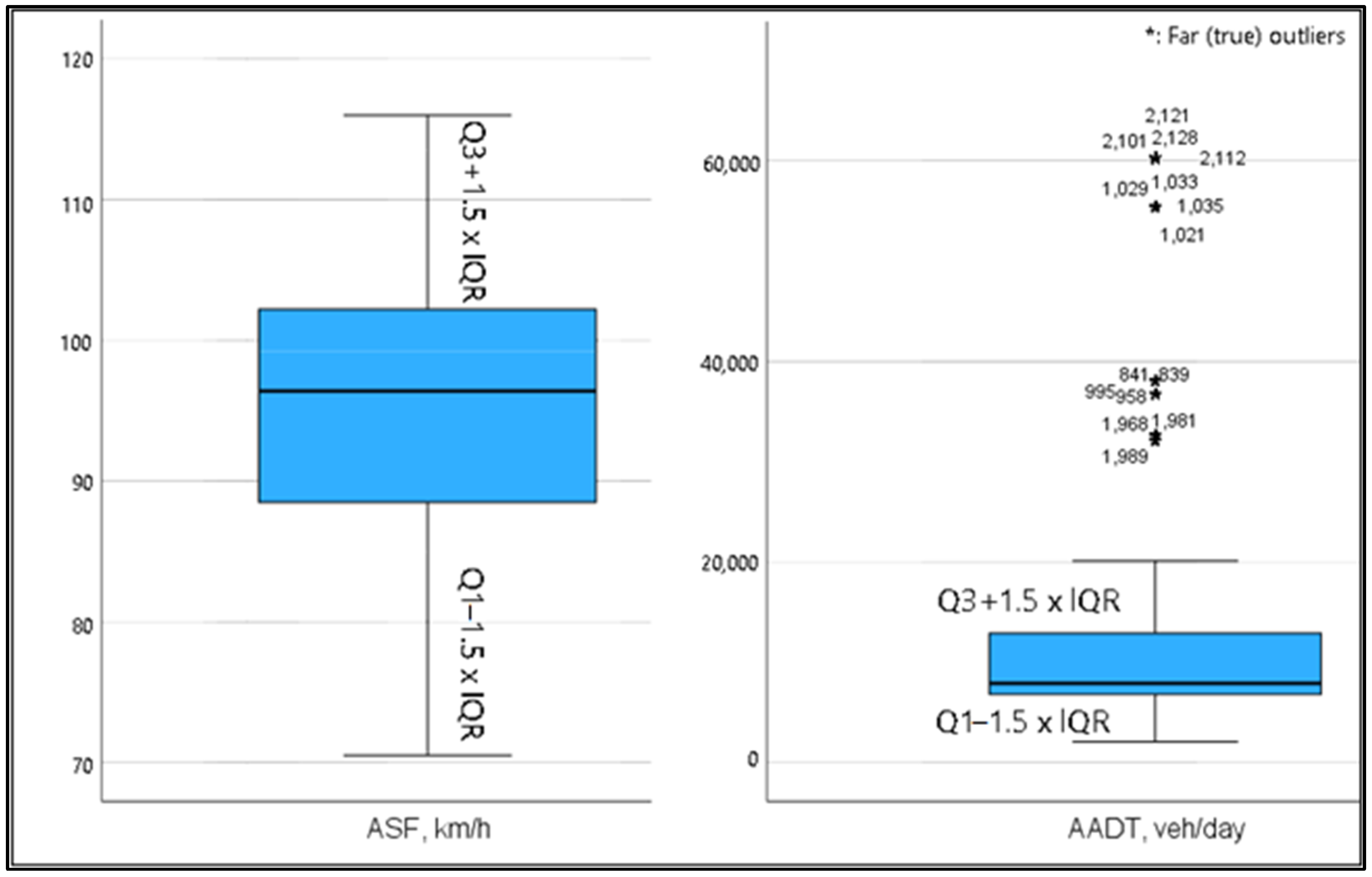
| ASF | 88.5 | 102.2 | 13.7 | −2.9658 > −2.698 * | 43 | 2.1715 < 2.698 * | N/A 2 |
| AADT | 6794 | 12,904 | 6110 | −0.8119 < −2.698 * | N/A 1 | 3.2333 > 2.698 * | 230 |
| Unweighted Cases | N | Percent | |
|---|---|---|---|
| Selected Cases | Included in Analysis | 3327 | 96.7 |
| Missing Cases | 112 | 3.3 | |
| Total | 3439 | 100.0 | |
| Unselected cases | 0 | 0.0 | |
| Total | 3439 | 100.0 | |
| Unweighted Cases | N | Percent | |
|---|---|---|---|
| RG1: Straight Section | Straight section (1) | 2344 | 70.5 |
| Other (0) | 983 | 29.5 | |
| RG2: Horizontal Curve | Horizontal curve (1) | 39 | 1.2 |
| Other (0) | 3288 | 98.8 | |
| Variable in the Equation | |||||||
|---|---|---|---|---|---|---|---|
| Model | B | S.E. | Wald | df | Sig. | Exp(B) | |
| Model 0 | Constant 1 | 1.055 | 0.040 | 709.766 | 1 | <0.001 | 2.873 |
| Predicted | |||||||
| CRTC | Percentage | ||||||
| Observed | Otherwise = 0 | Driver error = 1 | Correct 2 | ||||
| Model 0 | CRTC | Otherwise = 0 | 0 | 859 | 0.0 | ||
| Driver error = 1 | 0 | 2468 | 100.0 | ||||
| Overall percentage | 74.2 | ||||||
| Model | Chi-Square | df | Sig. | |
|---|---|---|---|---|
| Step 5 | Model 0 | 10.109 | 1 | 0.001 |
| Model 1 | 133.384 | 5 | <0.001 | |
| Predicted | ||||||
|---|---|---|---|---|---|---|
| CRTC | Percentage | |||||
| Observed | Otherwise = 0 | Driver Error = 1 | Correct 2 | |||
| Model 1 1 | CRTC | Otherwise = 0 | 16 | 843 | 1.9 | |
| Driver error = 1 | 7 | 2461 | 99.7 | |||
| Overall percentage/accuracy rate | 74.5 | |||||
| Coefficient | Std. Error | Wald | df | Sig. | ||
|---|---|---|---|---|---|---|
| Constant | 4.375 | 0.622 | 49.495 | 1 | <0.001 | 79.463 |
| NL | −0.501 | 0.101 | 24.782 | 1 | <0.001 | 0.606 |
| ASF | −0.027 | 0.005 | 28.831 | 1 | <0.001 | 0.973 |
| AADT. 10−3 | 0.016 | 0.005 | 12.580 | 1 | <0.001 | 1.017 |
| RG1 (Straight = 1) | 0.824 | 0.086 | 92.068 | 1 | <0.001 | 2.280 |
| RG2 (Horz.curve = 1) | 1.268 | 0.451 | 7.904 | 1 | 0.005 | 3.555 |
| Cut-Off Value | Observed | Predicted | Percent Correct | Accuracy (%) | Sensitivity (TPR) (%) | Specificity (1-FPR) (%) | Youden Index | ||
|---|---|---|---|---|---|---|---|---|---|
| 0 | 1 | ||||||||
| 0.60 | CRTC | 0 | 127 | 732 | 14.8 | 74.5 1 | 95.3 1 | 14.8 1 | 10.1 1 |
| 1 | 116 | 2352 | 95.3 | ||||||
| 0.59/ 0.58 | CRTC | 0 | 124 | 735 | 14.4 | 74.8 ↑ | 95.8 ↑ | 14.4 ↓ | 10.2 ↑ |
| 1 | 104 | 2364 | 95.8 | ||||||
| 0.55 | CRTC | 0 | 84 | 775 | 9.8 | 74.8 ↑ | 97.4 ↑ | 9.8 ↓ | 7.2 ↓ |
| 1 | 65 | 2403 | 97.4 | ||||||
| 0.50 | CRTC | 0 | 16 | 843 | 1.9 | 74.5  | 99.7 ↑ | 1.9 ↓ | 1.6 ↓ |
| 1 | 7 | 2461 | 99.7 | ||||||
: no change.| Coefficient | Wald | df | Sig. |
|---|---|---|---|
| Accident hour | 20.477 | 23 | 0.613 > 0.05 |
| Weekday | 5.187 | 6 | 0.520 > 0.05 |
| Month | 5.271 | 11 | 0.219 > 0.05 |
| Weather | 3.853 | 5 | 0.247 > 0.05 |
| Speed limit | 0.899 | 1 | 0.343 > 0.05 |
| Variables | VIF | NL | ASF | AADT. 10−3 | RG1 = 1 | RG2 = 1 |
|---|---|---|---|---|---|---|
| NL | 2.273 | 1.000 | ||||
| ASF | 1.349 | 0.245 | 1.000 | |||
| AADT. 10−3 | 2.148 | −0.658 | 0.133 | 1.000 | ||
| RG1 (Straight = 1) | 1.049 | −0.012 | −0.132 | 0.023 | 1.000 | |
| RG2 (Horz.crv = 1) | 1.031 | −0.036 | −0.021 | 0.019 | 0.121 | 1.000 |
| Model | AUC | Accuracy (CA) | Balanced Accuracy (BAC) | F1 1 | Precision | LogLoss |
|---|---|---|---|---|---|---|
| Dataset (1): 3439 cases (no data imputing) and models were tested using 10-fold cross-validation. | ||||||
| RF 2 | 0.701 | 0.760 | 0.593 | 0.853 | 0.787 | 0.512 |
| kNN 3 | 0.612 | 0.745 | 0.600 | 0.839 | 0.792 | 4.557 |
| BNLOGREG 4 | 0.607 | 0.747 | 0.500 | 0.855 | 0.747 | 0.548 |
| Dataset (2): Cases with missing values removed (69.44% data used) and models tested using 10-fold cross-validation. | ||||||
| RF 2 | 0.653 | 0.787 | 0.500 | 0.881 | 0.787 | 0.490 |
| kNN 3 | 0.595 | 0.724 | 0.556 | 0.829 | 0.809 | 2.365 |
| BNLOGREG 4 | 0.554 | 0.787 | 0.500 | 0.881 | 0.787 | 0.510 |
| Dataset (3): Model-based imputer (simple tree) used to replace missing values (100% data used), and models tested using 10-fold cross-validation. | ||||||
| RF 2 | 0.712 | 0.762 | 0.598 | 0.854 | 0.789 | 0.503 |
| kNN 3 | 0.643 | 0.755 | 0.547 | 0.851 | 0.794 | 2.154 |
| BNLOGREG 4 | 0.608 | 0.747 | 0.500 | 0.855 | 0.747 | 0.547 |
| Predicted | ||||||
|---|---|---|---|---|---|---|
| CRTC | Percentage | |||||
| Observed | Otherwise = 0 | Driver error = 1 | Correct | |||
| RF model 1 | CRTC | Otherwise = 0 | 229 | 640 | 26.4 | |
| Driver error = 1 | 178 | 2392 | 93.1 | |||
| Overall percentage/accuracy rate | 76.2 | |||||
Publisher’s Note: MDPI stays neutral with regard to jurisdictional claims in published maps and institutional affiliations. |
© 2022 by the authors. Licensee MDPI, Basel, Switzerland. This article is an open access article distributed under the terms and conditions of the Creative Commons Attribution (CC BY) license (https://creativecommons.org/licenses/by/4.0/).
Share and Cite
Akin, D.; Sisiopiku, V.P.; Alateah, A.H.; Almonbhi, A.O.; Al-Tholaia, M.M.H.; Al-Sodani, K.A.A. Identifying Causes of Traffic Crashes Associated with Driver Behavior Using Supervised Machine Learning Methods: Case of Highway 15 in Saudi Arabia. Sustainability 2022, 14, 16654. https://doi.org/10.3390/su142416654
Akin D, Sisiopiku VP, Alateah AH, Almonbhi AO, Al-Tholaia MMH, Al-Sodani KAA. Identifying Causes of Traffic Crashes Associated with Driver Behavior Using Supervised Machine Learning Methods: Case of Highway 15 in Saudi Arabia. Sustainability. 2022; 14(24):16654. https://doi.org/10.3390/su142416654
Chicago/Turabian StyleAkin, Darcin, Virginia P. Sisiopiku, Ali H. Alateah, Ali O. Almonbhi, Mohammed M. H. Al-Tholaia, and Khaled A. Alawi Al-Sodani. 2022. "Identifying Causes of Traffic Crashes Associated with Driver Behavior Using Supervised Machine Learning Methods: Case of Highway 15 in Saudi Arabia" Sustainability 14, no. 24: 16654. https://doi.org/10.3390/su142416654
APA StyleAkin, D., Sisiopiku, V. P., Alateah, A. H., Almonbhi, A. O., Al-Tholaia, M. M. H., & Al-Sodani, K. A. A. (2022). Identifying Causes of Traffic Crashes Associated with Driver Behavior Using Supervised Machine Learning Methods: Case of Highway 15 in Saudi Arabia. Sustainability, 14(24), 16654. https://doi.org/10.3390/su142416654