Impacts of Urbanization on Drainage System Health and Sustainable Drainage Recommendations for Future Scenarios—A Small City Case in China

Abstract

China is urbanizing at an unprecedented rate, but also accelerating the use of water resources and overloading of urban drainage systems. To analyze the impact of urbanization on the drainage-system health in Jinxi, a typical small case area in China, this study proposed an innovative methodological framework for evaluation and prediction based on statistical and modeling methods, which provides a demonstration and reference for urban development and drainage-system construction in developing countries. The result shows that the comprehensive urbanization index (CUI) of Jinxi shows an overall upward trend between 2009 and 2020. The drainage-system health index (DHI) shows a U-shaped trend of decreasing and then increasing, with the threshold in 2016. The years when the DHI and CUI are in balanced development occurred in 2014 and 2018. The impact of urbanization on the drainage-system health is divided into positive and negative aspects, depending on the drainage demands of the urban development. According to the predicted results, it is suggested that the next drainage upgrading measures will be favorable for sustainable urban development when the urbanization rate reaches 60%, the gross industrial output increases by 10%, or the total retail sales of consumer goods increase by 40%.

1. Introduction

Urbanization refers to the process of migration from rural to urban areas, accompanied by a gradual change in industrial structure from the primary to secondary and tertiary industries [1]. China is urbanizing at an unprecedented rate [2,3], which has risen from 17.9% in 1978 [4] to 64.7% in 2022 [5]. This rapid urbanization has promoted the social and economic development of China, but also accelerated the consumption of water resources and caused several water pollution problems [6], such as sewage pollution [7], industrial wastewater pollution [8], and non-point source pollution [9], which create tremendous pressure on the water resources and environment of China. Recently, the Chinese government has promulgated the Action Plan for Prevention and Control of Water Pollution [10], Sponge City [11], Three-year Action Plan for Improving the Quality and Efficiency of Urban Sewage Treatment (2019–2021) [12], and other policies to control and reduce water pollution. The essence of these measures is to upgrade and optimize the treatment capacity of the drainage system so that it remains balanced with rapid urbanization. Furthermore, the status of coordinated development of urbanization and drainage systems will contribute to the sustainability of the city and water environment. Therefore, it is urgent and of great scientific significance to explore the balanced development relationship between urbanization and drainage-system health and analyze the impact of urbanization on the drainage system.

According to the existing research, studies related to the impact of urbanization on drainage-system health can be broadly divided into three types. The first type evaluated the sustainable development of the city, where the drainage system was used as one of the evaluation indicators [13,14]. Generally speaking, a larger drainage scale and higher control rate of stormwater runoff indicate a higher level of sustainable urban development. The second type of study explored the coordination development of urbanization and the environment, where the outfalls in the drainage system were regarded as an indicator for point source pollution [4,15,16,17]. This type focused on the analysis of the processes of change in coordinated development and the key factors, population and economy, that contribute to environmental pollution. The third type was multi-system coupling analysis, which discussed the interactions between various sub-systems of urbanization, economy, energy, resources, and environment [18,19,20]. The conclusions of these studies were mostly consistent with the environmental Kuznets curve [1,21], which denotes a U-shaped relationship between urban development and the subsystems of environment, resources, and ecology. These studies mainly analyzed the national, regional, or large-scale metropolitan level. However, fewer studies focused on urbanization and drainage-system health in small-scale cities, limited by strategic importance and statistical data. Small cities, whose population is less than 200,000, are the mainstay of the urbanization process because of the huge population of rural residents. They are more prone to water pollution than modern cities due to the lack of attention to the scientific construction of drainage systems in the early stage of development [22].For example, the small cities or towns in China contain approximately 0.8 billion people, who are, more or less, facing drainage-system and water-pollution problems brought on by increased urbanization rates [23]. Therefore, this paper innovatively selects a typical small city as the research case to analyze the impact of urbanization on the drainage system, which is necessary for the sustainable development of urban drainage systems and water resources in developing countries.

For the small cities in whichever developing countries, there are four main development trends: the continued migration of the population from rural to urban areas [24], the transformation of agriculture from a scattered scale to a concentrated scale [25,26], the transformation of the industry from small scale to large scale [27], and the vigorous development of service industries relying on tourism resources [28,29,30]. Different small cities may choose the development plan corresponding to their conditions. As for Jinxi, it is a small city with the general development of primary, secondary, and tertiary industries, located in the east of Fuzhou, Jiangxi Province, China. It has not only a well-developed agricultural and spice industry as its economic base but also extremely abundant ancient villages as a tourist resource, which is why it has been called the Fragrance Capital and the Museum of Ancient Villages. Between 2009 and 2020, the proportion of the urban population in Jinxi increased from 31% to 48%, which is a critical stage of urbanization development. Considering the reality of Jinxi, it is a typical example of thousands of small cities in developing countries. With Jinxi as the study area, this paper provides a demonstration and reference for the coordinated development of urbanization and drainage systems in developing countries.

This study was divided into three steps. First, a novel index system for evaluating urbanization and drainage-system health was designed and applied based on the city statistical data and SWMM, a hydrological and hydraulic model. Then, the impact of urbanization on the drainage-system health was analyzed using correlation analysis. Finally, the Gray model was used to predict the changes in drainage-system health under different urbanization development scenarios in order to propose future-oriented urban-management suggestions for the balanced development of urbanization and drainage systems.

2. Study Area and Evaluation Index System

2.1. Study Area and Data Collection

Jinxi is located between 25°05’–27°40’ N and 116°25’–117°05’ E (Figure 1), and has 120,000 citizens on 2500 hectares. Data regarding urbanization and the drainage system were obtained from various sources, including Fuzhou Bureau of Statistics, Jinxi Bureau of Statistics, Jinxi Bureau of Natural Resources, Jinxi Bureau of Housing and Urban Development, and Google Images, etc. According to the Housing and Urban Development Bureau of Jinxi, a fundamental urban drainage-system upgrade project was carried out in 2017 and two new wastewater treatment plants (WWTP) began to operate in 2019. Since the earliest high-resolution remote-sensing images of Jinxi are from 2009, we chose the period of 2009–2020 as our study time interval. The list of data collection is shown in

Table 1. List of data collection.

Name	Years	Format	Source
Jinxi Statistical Yearbook	2010–2021	pdf/xls	Statistics Bureau, Fuzhou/Jinxi
Historical Remote Sensing Images	2009–2020	img/tif	KOMPSAT-2/Landsat 7/Landsat 8 /Google History Images
Digital Elevation Map (DEM)	2020	tif	Natural Resources Bureau, Jinxi
Historical Drainage system data	2010/2018	dwg	Housing and Urban Development Bureau, Jinxi
Hourly observation data of weather	2009–2010	txt	National centennial for environmental information, USA
Inflow data of WWTPs	2019	xls	Operation Office of WWTPs, Jinxi
Monitoring outfall data	2021	xls	Field experiments

.

2.2. Evaluation Index System

2.2.1. Comprehensive Urbanization Index

Generally, the urbanization rate is the proportion of the urban population to the total population [31], which does not satisfy a comprehensive evaluation. Recently, researchers have proposed a methodology to establish a scientific and comprehensive system of indicators to evaluate the urbanization process [4,19,20]. In this study, we referred to the existing evaluation system and selected 24 indicators to evaluate the urbanization process in four dimensions: population, social development, economy, and spatial development (

Table 2. The urbanization evaluation index and weights of indicators.

Dimensions	Indicators	Code	Unit	Property	Subjective Weight	Objective Weight	Comprehensive Weight
Population	Urbanization rate	X1	%	Positive	0.313	0.034	0.175
	Population density	X2	/km2	Positive	0.104	0.043	0.076
	Total				0.417	0.077	0.251
Social development	Consumer price index	X3	-	Positive	0.025	0.045	0.037
	Years of education per capita	X4	year	Positive	0.008	0.045	0.028
	Municipal sweeping area	X5	ha	Positive	0.004	0.042	0.025
	Number of beds in health institutions	X6	-	Positive	0.018	0.041	0.031
	Total gas supply	X7	thousand m3	Positive	0.006	0.033	0.021
	Total water supply	X8	thousand m3	Positive	0.011	0.043	0.029
	Disposable income per capita	X9	¥	Positive	0.018	0.042	0.032
	Total				0.090	0.291	0.203
Economy	GDP	X10	billion ¥	Positive	0.128	0.043	0.087
	Gross industrial output	X11	billion ¥	Positive	0.089	0.044	0.068
	Total retail sales of consumer goods	X12	billion ¥	Positive	0.025	0.043	0.036
	The proportion of the population in the secondary industry	X13	%	Positive	0.051	0.041	0.048
	The proportion of the population in the tertiary industry	X14	%	Positive	0.040	0.044	0.044
	Total				0.332	0.215	0.283
Spatial development	Urban built-up area	X15	ha	Positive	0.038	0.042	0.042
	The proportion of high-rise buildings	X16	%	Positive	0.030	0.044	0.039
	The proportion of low-rise buildings	X17	%	Negative	0.005	0.042	0.025
	The proportion of industrial land	X18	%	Positive	0.024	0.038	0.032
	The proportion of bare land	X19	%	Negative	0.005	0.043	0.026
	Proportion of road	X20	%	Positive	0.008	0.039	0.025
	The proportion of water surface	X21	%	Positive	0.016	0.042	0.031
	Proportion of woodland	X22	%	Positive	0.018	0.043	0.032
	Proportion of farmland	X23	%	Negative	0.009	0.045	0.029
	Proportion of river	X24	%	Positive	0.008	0.040	0.025
	Total				0.160	0.416	0.306

). The population is the core of urbanization, and all the urban activities serve the citizens [32]. Social development represents the vitality of the city, where citizens can enhance their quality of life through education, healthcare, and cultural activities [33,34]. The economy is the lifeblood and engine of the city driving the development of urbanization [35,36]. The spatial development represents the current status of the city. For example, the proportion of high-rise buildings relates to the aggregation of residents, the proportion of roads represents transportation development, the proportion of farmland represents agricultural development, the forest land and water surface represent ecological development, etc. [37,38,39]. Table 2 showed the composition and weights of the CUI.

Among the 24 indicators, X1–X15 were obtained directly from statistical yearbooks, and X16–X24 were calculated from the supervised classification of land use (LU) using remote-sensing images [40,41]. The specific details of each indicator are shown in Appendix A,

Table A1. The original data of the comprehensive urbanization index.

Indicators	2009	2010	2011	2012	2013	2014	2015	2016	2017	2018	2019	2020
X1	31.70	32.02	31.64	32.20	33.05	32.92	32.75	33.88	34.16	34.44	34.50	48.21
X2	4052	4140	4180	4320	4640	4664	4606	4717	4767	4810	4818	4894.92
X3	97.9	103.1	104.4	102.4	101.8	103.2	100.9	101.5	101.6	102.1	102.6	103.8
X4	12.25	13.1	14.22	14.89	15.07	15.11	15.63	15.71	15.79	15.59	15.22	15.53
X5	59	73	73	108	118	129	140	141	194	198	200	220
X6	492	622	622	622	622	622	660	673	919	985	995	1404
X7	15	16	27	26	13.4	13.6	13.8	14.1	14.12	14.3	14.4	14.8
X8	653	650	740	795	834.75	834.75	697.5	787.1	297.14	615	703	713
X9	14,503	16,240	17,903	18,649	20,168	22,102	23,914	25,875	28,662	30,237	32,634	34,599
X10	3.080	3.616	4.521	5.426	6.097	6.735	7.220	7.907	8.372	9.046	9.333	9.589
X11	2.527	3.828	4.709	5.229	7.412	9.122	9.986	10.698	7.916	6.090	6.133	6.533
X12	1.027	1.221	1.448	1.665	1.865	2.149	2.409	2.714	3.040	3.079	3.438	2.917
X13	6.34	6.78	7.49	8.02	8.13	17.33	17.56	17.53	15.87	16.85	17.03	20.49
X14	13.22	13.47	14.98	9.32	17.75	15.26	15.46	15.78	16.55	17.70	17.87	22.89
X15	12.00	12.25	12.11	13.25	13.75	14.00	14.40	14.80	14.85	15.10	15.20	15.60
X16	6.19	7.28	11.74	16.20	17.20	18.20	21.75	25.29	24.79	24.28	23.00	21.71
X17	11.31	16.01	18.08	20.14	22.39	22.45	23.19	23.73	24.75	22.27	22.43	23.82
X18	1.26	1.48	1.67	1.85	2.05	6.24	5.81	5.37	6.42	6.47	7.28	7.10
X19	3.72	4.38	2.38	0.39	1.84	3.30	4.92	6.55	5.67	4.79	4.85	4.91
X20	1.52	1.79	1.52	1.25	1.73	1.33	1.92	2.17	2.97	2.78	3.70	3.63
X21	2.13	2.50	2.10	3.71	4.54	4.37	4.78	6.14	6.60	6.06	6.41	5.76
X22	33.81	33.89	30.55	29.22	29.20	28.18	21.74	16.60	14.13	18.67	17.39	18.11
X23	36.61	28.60	29.50	26.40	19.78	14.23	14.70	13.45	13.67	13.38	14.03	14.44
X24	3.45	4.06	2.46	0.85	1.28	1.70	1.20	0.70	1.00	1.30	0.91	0.53

. The index weights were calculated using the analytic hierarchy process (AHP) and the entropy weight method (EWM), where the AHP generates the subjective weights of the experts and the EWM generates the objective weights of the index. The calculation process of AHP and EWM is shown in Section 3.2. The average of the subjective and objective weights represents the importance of the index.

In the four dimensions, the population had the highest subjective weight at 0.417 followed by the economy (0.332), spatial development (0.160), and social development (0.090), indicating that the population indicators and the economy indicators dominated for the experts who scored the weights. Spatial development had the highest objective weight at 0.416, indicating that it has the largest range of changes during 2009–2020. Overall, spatial development contributed the highest comprehensive weight, followed by the economy, population, and social development.

2.2.2. Drainage-System Health Index

We selected 12 indicators to evaluate the health of the drainage system in four dimensions: drainage-system scale, rainwater destination, pollution, and drainage system status. The drainage-system scale is the most visual indicator of the drainage system. Generally, the larger it is, the healthier the urban drainage system is. The rainwater-destination dimension measures the collection and conversion of rainwater, including the rate of infiltration and runoff. For the pollution dimension, we chose the total nitrogen (TN) as the representative pollutant and converted the runoff and overflow pollution into pollution per mm of precipitation, since precipitation is a vital factor impacting the amount of runoff and overflow pollution and we had to eliminate the effect of precipitation on runoff and pollution. The drainage-system-status dimension represents the overload and overflow of pipes and WWTP. The lower it is, the healthier the urban drainage system is.

Table 3. The drainage-system health index system and weights of indicators.

Dimensions	Indicators	Code	Unit	Property	Subjective Weight	Objective Weight	Comprehensive Weight
Drainage system scale	Pipes density	X25	km/km2	Positive	0.053	0.085	0.069
	The daily treatment capacity of WWTPs	X26	m3/d	Positive	0.053	0.037	0.045
	Total				0.106	0.122	0.114
Rainwater destination	Infiltration rate	X27	-	Positive	0.018	0.085	0.052
	Runoff rate	X28	-	Negative	0.091	0.090	0.091
	Total				0.109	0.175	0.142
Pollution	TN runoff pollution per mm of precipitation	X29	kg/mm	Negative	0.037	0.085	0.061
	TN point source pollution	X30	kg	Negative	0.062	0.088	0.075
	TN combined sewer overflow per mm of precipitation	X31	kg/mm	Negative	0.117	0.091	0.104
	TN outfall pollution per mm of precipitation	X32	kg/mm	Negative	0.333	0.087	0.210
	Total				0.549	0.351	0.450
Drainage system status	Overloaded sewage inflow of WWTPs	X33	m3/y	Negative	0.042	0.082	0.062
	Days of overloaded WWTPs	X34	d/y	Negative	0.015	0.089	0.052
	Total time of surcharge pipes	X35	h/y	Negative	0.040	0.091	0.066
	Total overflow of nodes	X36	m3/y	Negative	0.138	0.091	0.115
	Total				0.236	0.352	0.294

shows the composition and weights of the drainage-system health index. Among the 12 indicators, X25–X26 were obtained from the statistical yearbooks, and X27–X36 were simulated from the drainage-system model. The modeling methods of the drainage system are described in Section 3.1. Details of the drainage-system health index are shown in Appendix A,

Table A2. The original data of the drainage-system health index.

Indicators	2009	2010	2011	2012	2013	2014	2015	2016	2017	2018	2019	2020
X25	8.31	7.51	7.45	7.40	7.27	7.71	7.99	8.07	8.79	8.82	9.32	9.32
X26	20	20	20	20	20	20	20	20	20	20	30	30
X27	48.72	47.50	43.10	46.08	43.95	38.92	31.14	29.16	32.96	28.37	29.40	26.67
X28	41.97	45.87	45.10	42.63	47.04	48.84	47.65	48.60	53.13	51.63	55.81	57.31
X29	15.09	15.55	12.12	14.84	15.33	15.74	14.51	14.99	12.75	12.41	14.03	12.43
X30	6204	6367	6411	6677	6910	6939	8489	8515	8478	8476	9890	9905
X31	1672	1135	2356	1036	2118	1529	1401	1460	2096	2001	4254	4078
X32	1232	826	1746	751	1565	1121	932	971	1401	1337	1690	1622
X33	4531	4647	4690	4871	5051	5072	8303	8345	8323	8333	9957	12967
X34	60	82	122	120	165	160	182	195	203	222	125	160
X35	31,776	36,866	29,539	39,956	33,143	36,226	56,667	56,670	53,781	51,698	511,086	509,510
X36	33,367	50,127	22,759	59,928	30,131	39,520	54,049	56,432	36,662	37,420	97,186	93,651

. The difference in weights is also obvious between dimensions in the drainage-system health index (Table 3). Pollution had the highest subjective weight at 0.549 followed by drainage-system status (0.236), rainwater destination (0.109), and drainage-system scale (0.106). The objective and comprehensive weight of dimensions had the same rankings with different values.

3. Research Methods

We designed an evaluation index system of comprehensive urbanization and drainage system health. The statistical method, remote-sensing image analysis, and hydrology and hydraulic model were used to obtain the specific values of the indicators. The analytic hierarchy process and entropy methods were applied to perform subjective and objective weightings. The correlation analysis was carried out to explore the impact of urbanization on the drainage system. The gray system model [42] was used to predict the changes in drainage-system health indicators in different development scenarios. The technology roadmap is shown in Figure 2.

3.1. Calculation Methods for the Value of Indicators

3.1.1. Supervised Classification of Spatial-Development Indicators

Supervised classification, also known as training classification, is the process of using sample images from the identified category to identify unknown category images [43,44]. We used the object-oriented image-classification method in ENVI 5.3 (Exelis Visual Information Solutions Corporation, Colorado, United States) to extract the LU information from remote-sensing images of Jinxi, which were provided by KOMPSAT-2 (2009) and Google historical image (2011–2020). Each image was chosen to be sunny and cloudless, and taken in July or August. The image from KOMPSET-2 was bought and pre-processed from the Map Services Company (Shengshi Huayao Technology Corporation, Beijing, China). In addition, the images downloaded from Google historical images are provided from Landsat 7 and Landsat 8. The sample set consisted of nine types and 270 samples of LU, including high-rise buildings, low-rise buildings, industrial plants, rivers, water surface, farmland, woodland, roads, and bare land, which were manually labeled. The LU changes in the period of 2009–2020 are shown in Appendix A, Figure A1. The confusion matrix, especially the kappa coefficient, was used to evaluate the accuracy of LU classification [43,44]. According to Appendix A,

Table A3. The confusion matrix for LU classification.

	Output	High-Rise Buildings	Low-Rise Buildings	Industrial Plants	Rivers	Water Surface	Farmland	Woodland	Roads	Bare Land	Kappa Coefficient
Input
2009
High-rise buildings		24	2	3	0	0	0	0	0	1	0.80
Low-rise buildings		2	25	1	0	0	2	0	0	0
Industrial plants		0	0	26	0	1	2	0	0	1
Rivers		0	1	0	25	2	0	0	1	1
Water surface		0	0	0	0	27	2	0	0	1
Farmland		0	0	0	0	4	26	0	0	0
Woodland		0	0	0	0	1	2	24	1	2
Roads		0	0	0	5	0	3	0	21	1
Bare land		0	3	1	0	1	0	0	0	25
2012
High-rise buildings		26	2	1	0	0	0	0	0	1	0.83
Low-rise buildings		2	27	1	0	0	0	0	0	0
Industrial plants		0	1	29	0	0	0	0	0	0
Rivers		0	0	0	24	3	0	0	2	1
Water surface		0	0	0	0	24	2	3	0	1
Farmland		0	0	0	0	4	23	0	2	1
Woodland		0	0	0	0	1	2	24	1	2
Roads		0	0	0	2	0	0	1	26	1
Bare land		0	1	0	0	1	1	0	0	27
2014
High-rise buildings		24	2	1	0	0	0	0	0	3	0.82
Low-rise buildings		1	28	1	0	0	0	0	0	0
Industrial plants		0	2	27	0	0	0	1	0	0
Rivers		0	0	0	24	3	0	0	2	1
Water surface		0	0	0	0	24	2	3	0	1
Farmland		0	0	0	0	3	24	0	2	1
Woodland		0	0	0	0	1	2	24	1	2
Roads		0	0	0	3	0	0	1	25	1
Bare land		0	1	0	0	1	1	0	0	27
2016
High-rise buildings		25	2	1	0	0	0	0	0	2	0.88
Low-rise buildings		1	28	1	0	0	0	0	0	0
Industrial plants		0	1	29	0	0	0	0	0	0
Rivers		0	0	0	27	3	0	0	0	0
Water surface		0	0	0	0	27	2	0	0	1
Farmland		0	0	0	0	4	25	0	0	1
Woodland		0	0	0	0	1	0	26	1	2
Roads		0	0	0	2	0	0	1	26	1
Bare land		0	1	0	0	1	1	0	0	27
2018
High-rise buildings		25	2	1	0	0	0	0	0	2	0.85
Low-rise buildings		2	24	3	0	0	0	0	0	1
Industrial plants		0	1	29	0	0	0	0	0	0
Rivers		0	0	0	27	3	0	0	0	0
Water surface		0	0	0	0	25	2	2	0	1
Farmland		0	0	0	0	1	26	0	2	1
Woodland		0	0	0	0	1	2	25	1	1
Roads		0	0	0	2	0	0	1	25	2
Bare land		0	1	0	0	1	0	0	0	28
2020
High-rise buildings		28	0	1	0	0	0	0	0	1	0.84
Low-rise buildings		2	25	1	0	0	0	1	0	1
Industrial plants		0	1	27	0	2	0	0	0	0
Rivers		0	0	0	26	1	0	0	2	1
Water surface		0	0	0	0	24	2	3	0	1
Farmland		0	0	0	0	4	25	0	0	1
Woodland		0	0	0	0	1	2	24	1	2
Roads		0	0	0	2	0	0	1	26	1
Bare land		1	1	0	0	1	1	0	0	26

, the kappa coefficient of LU classification from each image was greater than 0.80, indicating that the classification results were acceptable.

3.1.2. Drainage-System Modeling

The drainage-system model was built on Stormwater Management Model (SWMM) [45]. Meanwhile, we used ArcGIS 10.7 to calculate the hydrology and hydraulic parameters that had to be input into the SWMM. The hydrology unit of SWMM had 709 subcatchments which were divided based on the high-resolution DEM data [46]. The hydraulic unit included the junctions, outfalls, conduits, pumps, and WWTPs, simulating the entire drainage network. The water-quality unit simulated 2 types of pollution input: rainwater washoff and wastewater inflow, which were the main pollution sources of the combined sewer overflow [47,48]. Horton infiltration formula was used to simulate the infiltration process [49,50,51]. For flow routing in the drainage network, the dynamic wave routing scheme was used. Evaporation rates and precipitation were simulated in SWMM based on the hourly observation data of weather, which were downloaded from the National Centers for Environmental Information. We built a series of updated SWMM models based on the collected data and supervised classification results of LU in different years, which represented 2010/2012/2014/2016/2018/2020, separately. The parameters were not always the same between models, as Jinxi kept developing. Therefore, the different inputs among the series of drainage models are shown in

Table 4. The different inputs among the series of SWMMs.

Items		Differences among the Series of Models
Hydrology unit	Precipitation	Hourly precipitation data per year
	Evaporation	Daily evaporation data per year
	Maximum infiltration rate	Depending on the type of soil and LU
	Manning coefficient	Depending on the type of soil and LU
	Percent of impervious	Depending on LU
Hydraulic unit	Drainage network	The drainage system was upgraded in 2017
	WWTP	Two new WWTPs were operated in 2019
Water quality unit	Wastewater discharge	Depending on the type of LU and the population
	Washoff	Depending on the type of LU

.

According to Table 4, the result of LU classification was used to assign the initial values to infiltration, Manning coefficient, wastewater discharge parameters, and washoff pollution. The initial value ranges of the hydrological parameters are shown in Appendix A,

Table A4. Hydrological parameter range and initial values.

Parameters	Unit	Type of LU	Range	Initial Values
Max infiltration rate	mm/hour	high-rise buildings, low-rise buildings, industrial plants, road	0~12.7	6.85
		river, water surface	9999	9999
		farmland, woodland	50–250	150
		bare land	25.4–127	70
Min infiltration rate	mm/hour	except bare land	0.25–10.99	2.54
		bare land	0.25–120	35
Decay constant	1/hour	all types	2~7	4
Drying time	day	all types	2~14	3
Manning coefficient	-	high-rise buildings, low-rise buildings, industrial plants, road	0.011–0.015	0.012
		farmland	0.06–0.17	0.1
		woodland	0.4–0.8	0.4
		bare land	0.01–0.05	0.05
		river, water surface	0	0
Depth of depression storage	mm	high-rise buildings, low-rise buildings, industrial plants, road	1.27–2.54	1.95
		woodland	7.62	7.62
		farmland	2.54–5.08	3.75
		bare land	2.54–7.62	5.08
		river, water surface	9999	9999

. The event mean concentrations washoff function were chosen for water-quality simulations in the drainage model [47,52] and different LU types correspond to different pollutant flushing coefficients, which are listed in Appendix A,

Table A5. Washoff parameter settings in different types of LU.

LU	Pollutant	Function	Co-efficiency	Street Cleaning Removal Efficiency/%
High-rise buildings	TN	EMC	0.005	85
Low-rise buildings	TN	EMC	0.012	60
Industrial plants	TN	EMC	0.002	75
Bare land	TN	EMC	0.008	50
Roads	TN	EMC	0.032	95
Water surface	TN	EMC	0	0
Woodland	TN	EMC	0.015	0
Farmland	TN	EMC	0.02	0
Rivers	TN	EMC	0	0

. Wastewater discharge is highly correlated with human activities and LU. In this case, we allocated the total amount of wastewater to each subcatchment according to the building area. The calculation formula is as follows:

$${\mathrm{Q}}_{\tau }=\frac{3\times S_{\tau -high}+10\times S_{\tau -plant}+S_{\tau -low}}{3\times S_{high}+10\times S_{plant}+S_{low}}\times Q_{total}$$

(1)

where $\tau$ means the order of subcatchments, ranging from 0~607; ${\mathrm{Q}}_{\tau }$ is the wastewater discharge baseline for each subcatchment, m³/d;$Q_{total}$ is the average daily wastewater treatment capacity, m³/d; $S_{\tau }$ represents the area of high-rise buildings, industrial plants, and low-rise buildings in each subcatchment, m²; S represents the total area of each type of LU, m². Depending on the height of the building, we assume that the baseline drainage of a high-rise building is three times more than that of the low-rise building, and the industrial plant is about ten times. Furthermore, random factors between 0.7 and 1.3 were chosen randomly and multiplied with the baseline flow to simulate the real drainage process.

The minimum unit of calculation for the hydrologic process is the subcatchment in SWMM. When various types of LU exist in one subcatchment, it is necessary to provide the proportion for each type. In that case, the parameters were set according to the largest LU area of this subcatchment. After setting and running the initial model, the cross-validated method [53] was used in the calibration and verification of hydrological, hydraulic, and water-quality units. We monitored the flow of outfalls from five actual storms from 2019 to 2021, and used four of them for calibration and the rest for verification, repeating five times ordinally. The calibrated model simulated storm events with Nash-Sutcliffe efficiency values ranging from 0.73 to 0.93. We selected the calibration result with the highest Nash coefficient as the model parameter input. The calibration and verification data for the water-quality unit was obtained from the WWTP inlet data from January to December 2019, and the Nash–Sutcliffe efficiency was 0.82, which fit the requirements of accuracy.

3.2. Calculation Methods for the Weight of Indicators

The data should be normalized considering the differences in dimension, magnitude, and symbols [15,19]:

$$\mathrm{For} \mathrm{positive} \mathrm{indicators}: {\mathrm{X}}_{ij}=\frac{x_{ij}-x_{imin}}{x_{imax}-x_{imin}}$$

(2)

$$\mathrm{For} \mathrm{negative} \mathrm{indicators}:{ \mathrm{X}}_{ij}=\frac{x_{imax}-x_{ij}}{x_{imax}-x_{imin}}$$

(3)

where i is the serial number of the indicators; j represents the number of years; X_ij represents the normalized value and $x_{ij}$ represents the original value; and $x_{imax}$ and $x_{imin}$ represent the maximum and minimum value of the indicator x_i. The values of all indicators were normalized between 0 and 1 after the pre-processing.

The analytic hierarchy process (AHP) is a multi-criteria decision-making method, which was first introduced in the 1970s and has been widely applied to solve multi-objective complex problems [54,55]. In this study, we used YAAHP [56], an AHP software, to calculate the subjective weights of urbanization and drainage-system health index. The calculation process of AHP consists of 3 steps: (1) build a hierarchical model based on the relationship of indicators in Table 2 and Table 3; (2) obtain the judgment matrix from the experts who are from the executive managers of drainage-network department, Shenzhen Water Group; (3) input the judgment matrix into the YAAHP and conduct the consistency check to make sure the consistency index is below 0.1; and (4) output the subjective weights.

The entropy weight method (EWM) is a weighting method that calculates the objective weight of the indicator according to the dispersion degree of the data [57,58]. The required original data for the entropy method is shown in Appendix A, Table A1 and Table A2. In addition, the calculation process of EWM consists of three main steps, as follows.

(a)

Data normalization

$$P_{ij}=\frac{X_{ij}}{{{\displaystyle \sum }}_{j=1}^n{X}_{ij}}$$

(4)

(b)

Entropy calculation

$${\mathrm{E}}_i=-\ln \frac{1}{n}\times {\displaystyle \sum }_{j=1}^n\left(P_{ij}\times \ln P_{ij}\right)$$

(5)

where i is the serial number of the indicators; j represents the number of years; n represents the number of total years; and ${\mathrm{E}}_i$ represents the entropy of X_i.

(c)

Weight calculation

$$W_i=\frac{1-{\mathrm{E}}_i}{m-{{\displaystyle \sum }}_{i=1}^m{\mathrm{E}}_i}$$

(6)

where m represents the number of total indicators; and $W_i$ represents the objective weight of X_i.

3.3. Correlation Analysis and Principal Component Analysis

3.3.1. Correlation Analysis

The Pearson correlation coefficient (PCC) can be used to represent the correlation between two variables [59]. In general, the absolute value of PCC is considered to be a strong correlation between the two variables if it is greater than 0.8. A range between 0.3 to 0.8 is considered a weak correlation. There is considered to be no correlation when it is less than 0.3 [60]. We calculated the PCCs and validated the significance level using R studio in this study.

3.3.2. Principal Component Analysis

The 24 indicators of CUI were transformed into mutually independent variables by principal component analysis considering the correlation between the indicators of CUI. The principal component analysis [61,62] was finished with SPSS 26.0 and the results are shown in Appendix A,

Table A6. Total variance explained of CUI.

Components	The Initial Eigenvalues		Cumulative Variance Contribution Rate (%)	Extracting Square Loaded		Cumulative Variance Contribution Rate (%)
	Totals	Variance Contribution Rate (%)		Totals	Variance Contribution Rate (%)
1	13.371	55.712	55.712	13.371	55.712	55.712
2	4.443	18.513	74.225	4.443	18.513	74.225
3	2.784	11.602	85.827	2.784	11.602	85.827
4	1.560	6.500	92.328	1.560	6.500	92.328
5	0.746	3.107	95.434
6	0.449	1.870	97.305
7	0.281	1.172	98.477
8	0.181	0.753	99.230
9	0.120	0.500	99.730
10	0.043	0.179	99.908
11	0.022	0.092	100.000

. From Table A6, the cumulative variance contribution rate of the first four factors is 92.328%, indicating that the first four factors could well represent the main information from the 24 indicators. The factors were then extracted by the principal factor analysis method and the matrix is listed in Appendix A,

Table A7. Component score coefficient matrix of CUI.

Components	F1	F2	F3	F4
Urbanization rate	0.045	−0.093	0.056	0.351
Population density	0.073	0.012	0.038	−0.021
consumer price index	0.016	−0.004	0.217	0.301
Years of education per capita	0.064	0.067	0.121	−0.108
Municipal sweeping area	0.070	−0.057	0.061	−0.057
Number of beds in health institutions	0.056	−0.125	0.088	0.150
Total gas supply	−0.042	−0.005	0.253	−0.012
Total water supply	0.003	0.182	0.124	0.180
Disposable income per capita	0.070	−0.069	0.051	−0.017
GDP	0.073	−0.025	0.062	−0.068
Gross industrial output	0.052	0.146	−0.047	−0.050
Total retail sales of consumer goods	0.070	−0.033	0.036	−0.152
The proportion of population in secondary industry	0.071	0.005	−0.040	0.021
The proportion of population in tertiary industry	0.056	−0.072	−0.024	0.265
Urban built-up area	0.073	−0.011	0.032	−0.067
Proportion of high-rise housing	0.069	0.032	0.059	−0.197
Proportion of low-rise dwellings	−0.062	0.103	0.092	0.013
Proportion of industrial land	0.022	0.198	−0.118	−0.015
Proportion of bare land	−0.046	0.067	0.220	0.091
Proportion of road	0.036	0.170	−0.119	0.144
Proportion of water surface	0.035	0.124	−0.095	0.386
Proportion of forest	−0.053	−0.138	−0.027	0.126
Proportion of farm land	0.041	−0.075	−0.256	0.077
Proportion of river	−0.059	−0.055	−0.159	0.107

. The indicators of CUI were transformed into four mutually independent variables F1–F4, as follows:

$$\mathrm{F}1=0.045x_1+0.073x_2+0.016x_3+···+0.041x_{23}-0.059x_{24}$$

(7)

$$\mathrm{F}2=-0.093x_1+0.012x_2-0.004x_3+···-0.075x_{23}-0.055x_{24}$$

(8)

$$\mathrm{F}3=0.056x_1+0.038x_2+0.217x_3+···-0.256x_{23}-0.159x_{24}$$

(9)

$$\mathrm{F}4=0.351x_1-0.021x_2+0.301x_3+···+0.077x_{23}+0.107x_{24}$$

(10)

3.4. Future Scenarios Design and Prediction

3.4.1. Principles of Scenario Design

We set up four future scenarios to explore the impact of urbanization on drainage-system health in the future based on the actual indicator data of 2020, which were population development, industrial development, cultural and tourism development, and passive development. The population development scenario represented a normal urbanization mode characterized by the simultaneous development of social, economy, and spatial layout along with population growth. The industrial development scenario meant the future development of the secondary industry. The cultural and tourism development scenarios represented the future development of tertiary industry. The passive development scenario referred to the fact that the residents in small cities were attracted to the nearby large cities that can provide more opportunities and higher salaries, which is also called the Siphon Phenomenon in City Cluster [63,64]. There are 2 large cities, Fuzhou and Nanchang, surrounding Jinxi, which are attractive workplaces. The principles of scenario design are shown in

Table 5. Details of different scenarios.

Scenarios	Principles and Description
Population development	The urbanization rate increased from 0.48 to 0.50/0.55/0.60/0.65/0.70 and other indicators were adjusted synchronically according to the changes.
Industry development	The gross industrial output improves 10%/20%/30%/40%/50% of basic value, and other indicators were adjusted synchronically according to the changes.
Cultural and tourism development	The total retail sales of consumer goods improve 10%/20%/30%/40%/50% of basic value, and other indicators were adjusted synchronically according to the changes.
Passive development	The GDP declines −5%/−10%/−15%/−20%/−25% of basic value, and other indicators were adjusted synchronically according to the changes.

.

3.4.2. Method of Scenario Prediction

The gray system model has attracted wide attention due to its simplicity and efficiency in time-series prediction with small samples [42,65,66]. In this study, the gray model was chosen as the prediction method, which predicted the four dimensions of DHI with or without the upgrading measures, respectively. Indicator data from 2009–2015 were used to train the gray models without optimization measures of the drainage system, and data from 2016–2020 were applied for training the gray models with measures. For each gray system model, the inputs were the independent indicators F1–F4 calculated by principal component analysis, and the first-order accumulative generation operation (abbreviated as 1-AGO) data of the original series were used as accumulation. The outputs were the DHI prediction values for the future scenarios with and without the drainage upgrade measures, respectively. The relative error was used to assess the accuracy of the gray models. After calibrating the parameters, the relative error of each gray model was controlled within 20%.

4. Results and Discussion

4.1. Trends of CUI and DHI

The temporal changes in the CUI in Jinxi are shown in Figure 3a. The CUI presents an overall upward trend during 2009–2020, showing the similarity from other cities in developing countries [16,21,67,68]. The CUI maintains a steady development in 2009–2014 with the population, economy, society, and spatial development but decreased slightly during 2016–2018. The main reason for the decline is the spatial-development dimension. According to Table A1 and Figure A1, the rapid expansion of urban areas caused changes in the proportion of LU. During 2016–2018, about 7% of the land was developed from forest to residential and bare land, which was an inappropriate urbanization process, being at the expense of ecological resources. In 2019–2020, the CUI further increased as the population of Jinxi rapidly grew.

Figure 3b shows the changes in the DHI in Jinxi from 2009–2020 with an overall trend of decreasing in 2009–2015 and increasing in 2016–2020, which presents a U-shaped curve. The decline in DHI was caused by a combination of changes in the four dimensions. First, the drainage-system scale is lagging compared to the rapid urbanization during 2009–2015, resulting in a decrease in the drainage-system-scale dimension score. Second, the urbanization process caused pervious areas to be replaced by impervious areas, resulting in an increase in stormwater runoff, that is, a decrease in the stormwater-destination dimension. In addition, the increase in domestic and industrial water consumption increased the pollution discharge and drainage-system loading. After 2017, the DHI improved as the government recognized the problems in drainage systems and implemented upgrading measures, including the construction of drainage pipelines and wastewater treatment plants.

Figure 3c describes the development relationship between CUI and DHI in the period of 2009–2020. θ of the polar system is the angle between the point (CUI, DHI) and the origin, reflecting the degree of balanced development between urbanization and drainage-system health. When θ exceeds 45°and the value of DHI is greater than CUI, the drainage-system health is ahead of the urbanization development, which can be interpreted as the drainage system still having a surplus wastewater treatment capacity. Conversely, it indicates that urban development is ahead of the drainage-system health when θ is less than 45°. Therefore, Figure 3c is divided into two parts that are the drainage-leading area (DLA) and the urbanization-leading area (ULA). Jinxi is in the DLA during 2009–2014. However, the leading of drainage-system health gradually decreases as the CUI rises during this period. In 2014, the urbanization and drainage-system health reached a low-level balanced development. Jinxi has been in the ULA since 2015. In 2018, urbanization and drainage-system health are a high-level balanced development as the drainage-system upgrading project increased the DHI.

4.2. Impact of Urbanization on Drainage System Health

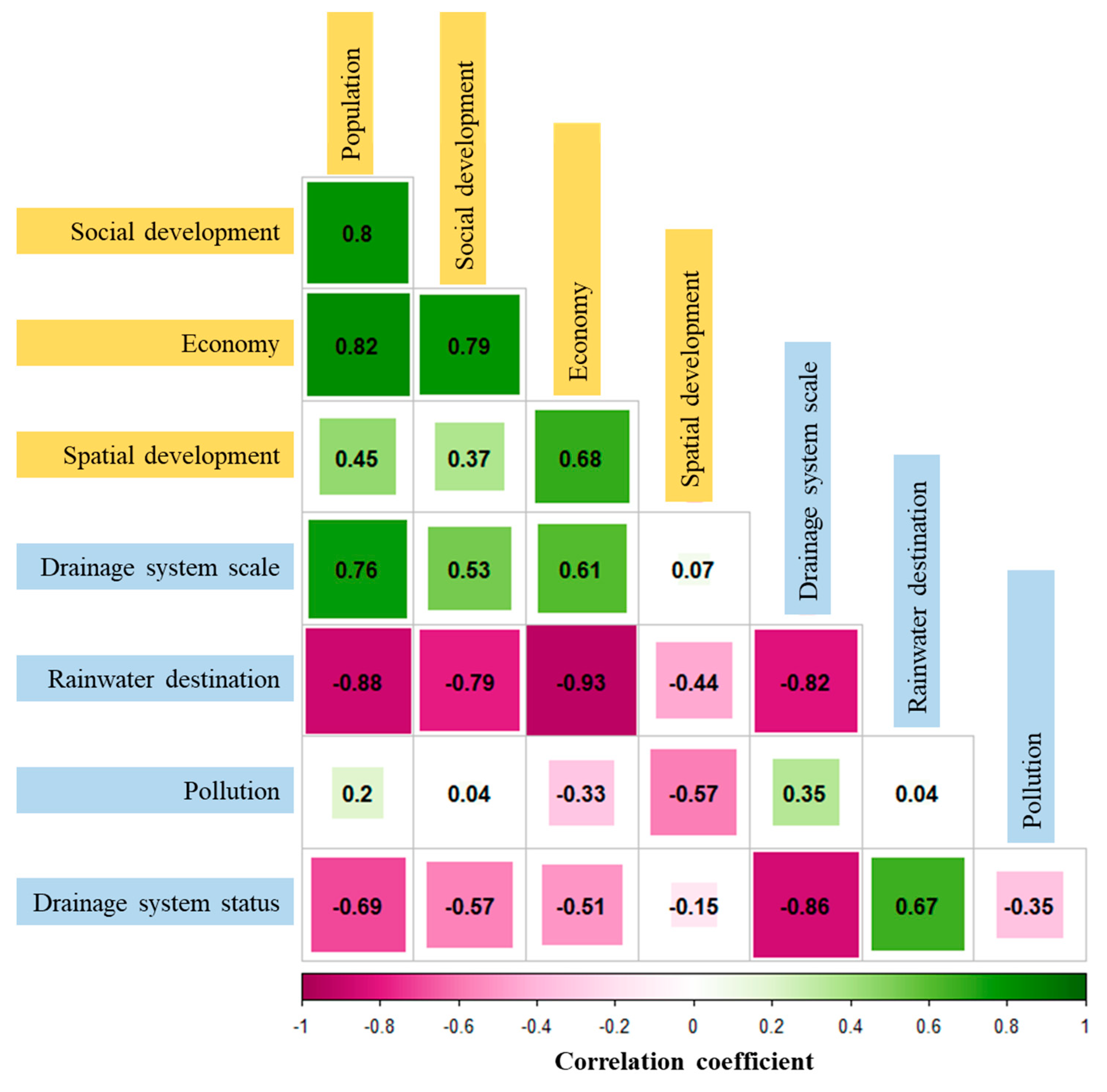
4.2.1. Correlation Analysis

The PCC is used to present the correlation between urbanization and drainage-system health. Figure 4 shows the heat map of the correlation coefficients for the eight dimensions of CUI and DHI, where green represents positive correlation and pink represents negative correlation. The four dimensions of the CUI show positive inner correlations with correlation coefficients varying from 0.37 to 0.82 in the top left corner of Figure 4. The inner correlation coefficients of the four dimensions of the DHI range from −0.86 to 0.67 located in the bottom right corner of Figure 4, where the drainage-system scale appears a strong negative correlation with the two dimensions: rainwater destination (−0.82) and drainage-system status (−0.86). As for the impacts of urbanization on drainage-system health, the population, social development, and economy have positive impacts on the drainage-system scale with coefficients of 0.76, 0.53, and 0.61, indicating that the scale of the drainage system is consistently increasing with the development of the urban population, society and economy. All of the dimensions of CUI have negative impacts on the rainwater destination, with coefficients of −0.88, −0.79, −0.93, and −0.44, respectively. This situation occurs because there is no measure of runoff control in Jinxi and the surface runoff creates immense pressure on the drainage system. The economy and spatial development have negative impacts on the pollution dimension with coefficients of −0.33 and −0.57, meaning that economic and spatial development leads to an increasing amount of pollution emissions in the natural environment. The population, social development, and economy have negative impacts on the drainage system status with coefficients of −0.69, −0.57, and −0.51, suggesting that urbanization development increases negative pressure on the operation of the drainage system. All the values pass the significance test at the level of 0.05.

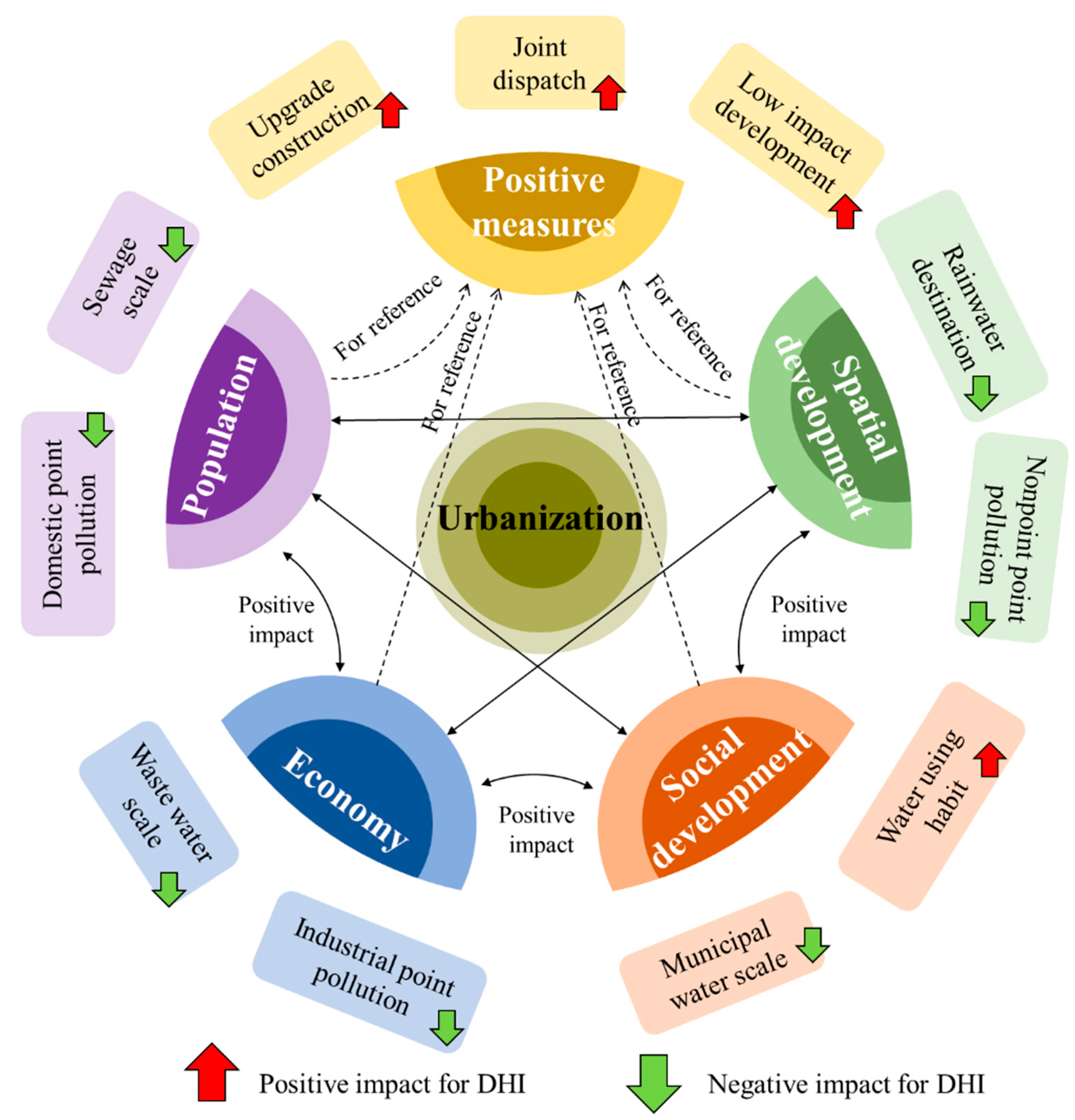
4.2.2. Qualitative Analysis and Mechanism

The results of the DHI trend are directly influenced by the various water-use habits of urban residents and the operation of the drainage system. Figure 5 shows the mechanism of the qualitative impact of urbanization on the drainage-system health. From the result of Section 4.1 and some related research, the impact is divided into negative and positive parts. The negative impact comes from the pressure of urbanization on the drainage system, such as increased domestic sewage due to population development, increased industrial sewage due to economy development, increased municipal water use due to social development, and increased stormwater runoff rates due to the large-scale development of the impervious area, which are shown as the green arrows in the outer ring of Figure 5. The positive impact comes from positive measures that can enhance the drainage-system health, such as drainage-system construction, low-impact development [69], joint dispatch of drainage systems [70], and promotion of water-saving behaviors [71,72,73], etc., which are shown as the red arrows in the outer ring of Figure 5. Changes in DHI are caused by a combination of positive and negative impacts. Jinxi experienced negative impacts at the beginning of the urbanization development process and positive impacts at the later stage, which can explain the U-shaped trend of Jinxi DHI in Section 4.1.

In the inner ring of Figure 5, there are several dashed lines connecting the four dimensions of urbanization and the positive measures of the drainage system, meaning that changes in the various dimensions of urbanization also provide references to the decision-making process for urban drainage-system upgrading measures. According to the correlation calculation results in Section 4.2.1, the economy dimension has the strongest correlation with the DHI among the urbanization dimensions, followed by the spatial, social, and population. Therefore, it would be more conducive to the sustainability of decision-making if the demands from the economy and spatial development were prioritized.

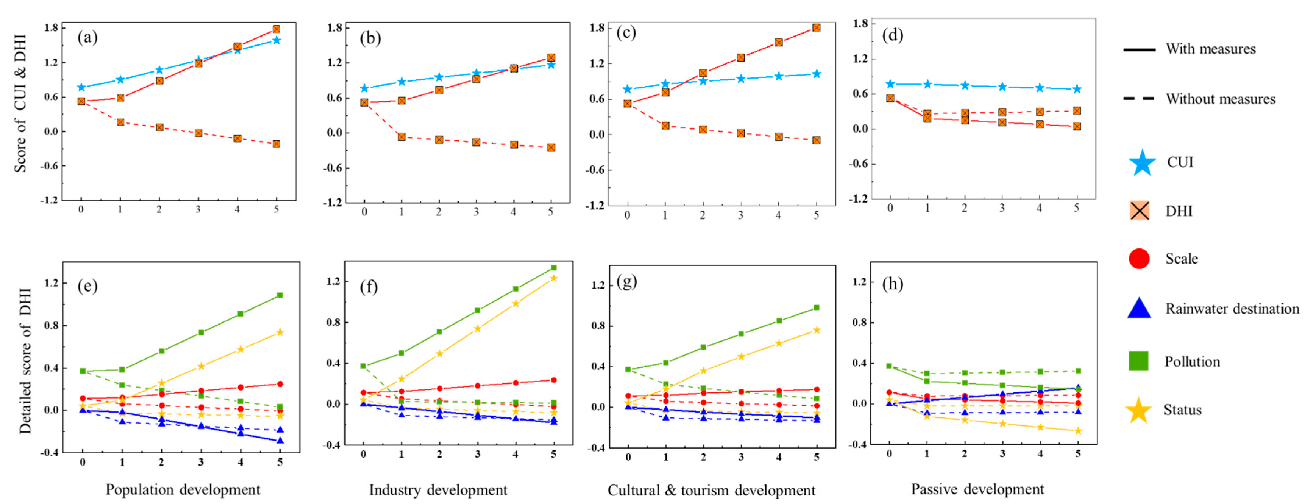
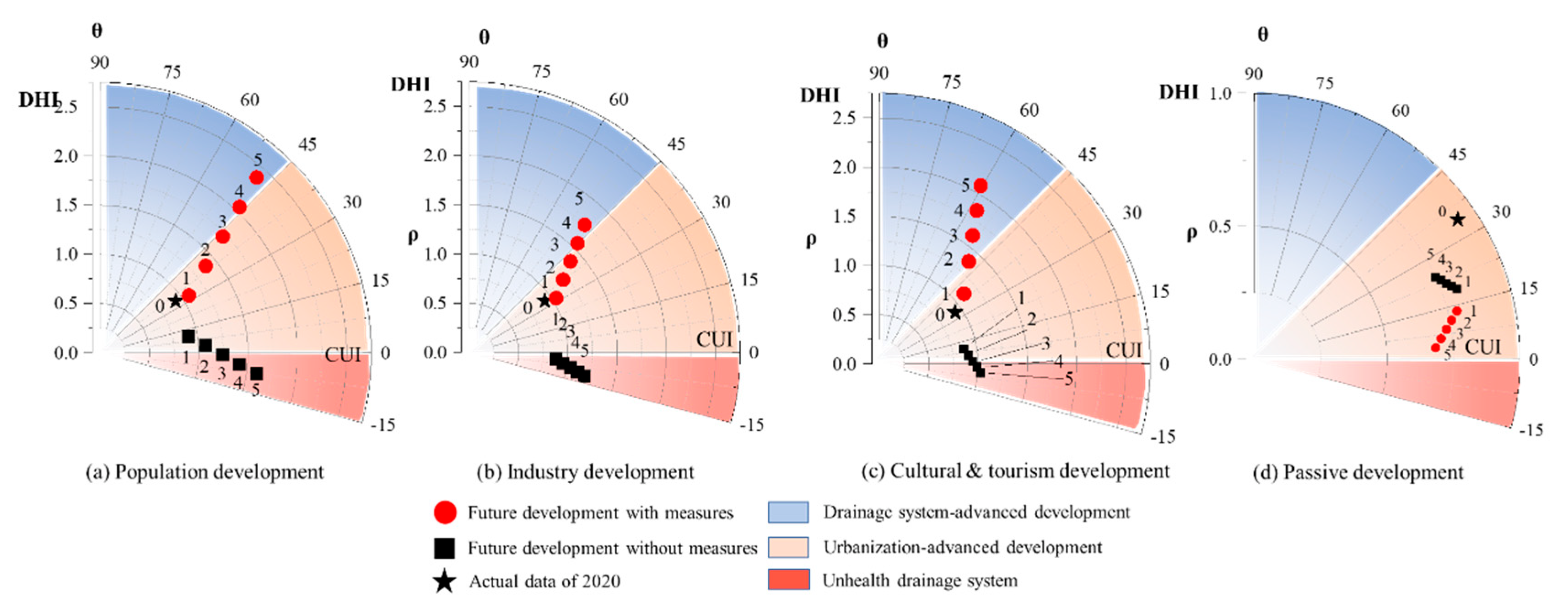
4.3. Future Scenarios Prediction

Figure 6a–d illustrates the prediction result of CUI and DHI for Jinxi in different scenarios, where each scenario includes two results for adopting drainage-system upgrading measures or not. Here, “0” on the x-axis represents the actual score of CUI and DHI in 2020, and “1”–“5” represents the intensities of the scenario. The predicted results of DHI have similar trends in the population (Figure 6a), industrial (Figure 6b), and cultural and tourism (Figure 6c) development scenarios. In the case of taking measures to upgrade the drainage system, DHI will increase with CUI, which means they can develop synergistically in a balanced relationship. On the contrary, if the government does not pay attention to the drainage-system health, DHI will decrease as the CUI increases, indicating that the drainage system of Jinxi will be gradually unbefitting of the growing demand of urbanization and probably lead to urban flooding and water-pollution problems. In the passive development scenario (Figure 6d), CUI and DHI will be decreasing with increasing development intensity. The passive development scenario is somehow like the inverse process of the population development scenario, where the population loss becomes more severe as the intensity of the scenario increases. As a result, the trend in Figure 6d shows the opposite to that in Figure 6a.

In addition, Figure 5e–h plots the detailed trends of the four dimensions of the DHI for each scenario, where different shapes represent the four dimensions in the legend. The score of scale, pollution, and status would be improved by taking drainage-network upgrade measures, meaning that the measures could significantly affect these three dimensions. The score of rainwater destinations would decrease (Figure 6e) or be essentially constant (Figure 6f,g) by adopting drainage-system upgrade measures, indicating that the measures are not the major factor. The ranking of the impact of drainage-system upgrading measures on the four dimensions could be analyzed according to the difference between the scores of measures and no measure: pollution > status > scale > rainwater destination. The trend of the scale, rainwater destination, and pollution in the passive development scenario is the opposite of the other three scenarios and the trend of the status is similar (Figure 6h). In this case, the overflows of the drainage system and overloads of WWTPs would be significantly reduced, leading to an upward trend in the drainage-system health status.

4.4. Suggestions for the Development of the Drainage System in Jinxi

Figure 7 shows the future development relationship between CUI and DHI based on the predicted results. Compared with Figure 3c, there exist negative numbers of θ in Figure 7, which means that some indicators of DHI are lower than the lowest score from 2009-2020. In another way, the drainage system will be in a terribly unhealthy state if the score of DHI is less than zero. Therefore, Figure 7 is divided into three areas by θ as 0 and 45°, which are the drainage-leading area (DLA), the urbanization-leading area (ULA), and the unhealthy area (UHA). Suggestions of drainage-system development for Jinxi are proposed based on the status area of different scenarios, as follows.

In the population development scenario, drainage upgrading measures will be recommended when the urbanization rate is up to 60%. The expected result will be a balanced development in CUI and DHI with θ = 43.55° (Figure 7a).

In the industry development scenario, it will be suggested to propose drainage upgrading measures when the gross industrial output improves by 10%. The expected result will still prioritize the urbanization development area with θ = 32.27°. According to the results in Figure 7b, the dimension of pollution is the main factor that causes the decrease in DHI. Therefore, the pre-treatment devices for industrial drainage should be the additional measures cooperating with drainage upgrading measures to reduce the quantity of pollution and improve the DHI score.

In the culture and tourism scenario, the measures to upgrade the drainage system will be favorable for sustainable urban development when the total retail sales of consumer goods improve by 40%, of which the expected result will be a priority of the drainage development area with θ = 57.68°. Therefore, the drainage-network upgrade measure is oversaturated in this scenario. According to Figure 7c, it is recommended that the drainage upgrading measure in level 2 be implemented instead of the measure in level 4 for the balanced development of CUI and DHI with θ = 49.00°.

In the passive development scenario, θ is always located in the ULA, which ranges from 18.99° to 24.32° (Figure 7d). Considering that the drainage-system pressure is also decreasing under the scenario, there is no need to implmement drainage-system upgrading measures for the time being. The current focus should be on considering how to reduce the impact of the urban siphon phenomenon and attract talents and quality investment for society and economic recovery. The balanced development of urbanization and drainage health would be considered when the city is back to its usual stage.

The low-impact development and joint dispatch of drainage systems are also important positive measures to improve the score of drainage-system health from Figure 4, though it has not been applied in Jinxi yet. Therefore, it is recommended that Jinxi should take a variety of positive measures in the future to maximize the score of the drainage-system health index and ensure the constant balanced development between urbanization and drainage-system health.

5. Conclusions

Taking Jinxi, a typical small city in developing countries, as an example, we evaluated the score of CUI and DHI from 2009 to 2020 and analyzed the impact of urbanization on drainage-system health. Then, we predicted the trends of DHI in four different development scenarios and made suitable suggestions for the drainage-system development of Jinxi. The conclusions are as follows. CUI increased overall but there was a slight decrease in 2017 and 2018 because of the inappropriate land development in the city. The changes in DHI showed a U-shape, decreasing first and then improving due to the drainage-system upgrading measures. According to the trend of CUI and DHI, 2014 and 2018 are the years of balanced development of urbanization and drainage-system health. The impact of urbanization on the drainage system is divided into negative and positive impacts. The negative impact comes from various drainage pressures during the development of urbanization, and the positive impact comes from various drainage-system management measures. This study focused on the impact of the current drainage-system upgrade measures on each dimension of DHI, which was ranked as pollution > status > scale > rainwater destination. Further drainage upgrading measures are favorable for sustainable development when the urbanization rate reaches 60%, the gross industrial output increases by 10%, or the total retail sales of consumer goods increase by 40%. If Jinxi faces the passive development scenario in the future, it could consider counteracting the attraction of large cities compared to nearby small cities before focusing on drainage-system health.

Admittedly, this work has the disadvantages of few study areas and uncertainty in model prediction. In the future, we will optimize the research method, such as by using the fractional multivariate gray model with convolutional integration [74] to replace the traditional gray model and apply it to other cities to explore and compare the different regular impacts of urbanization on drainage-system health.

References

1. Liang, W.; Yang, M. Urbanization, economic growth and environmental pollution: Evidence from China. Sustain. Comput. Inform. Syst. 2019, 21, 1–9. [Google Scholar] [CrossRef]
2. Shen, L.; Shuai, C.; Jiao, L.; Tan, Y.; Song, X. A Global Perspective on the Sustainable Performance of Urbanization. Sustainability 2016, 8, 783. [Google Scholar] [CrossRef] [Green Version]
3. Farrell, K.; Nijkamp, P. The evolution of national urban systems in China, Nigeria and India. J. Urban Manag. 2019, 8, 408–419. [Google Scholar] [CrossRef]
4. Liang, L.; Wang, Z.; Li, J. The effect of urbanization on environmental pollution in rapidly developing urban agglomerations. J. Clean. Prod. 2019, 237, 117649. [Google Scholar] [CrossRef]
5. China NBOS. The Total Population Has Increased and the Rate of Urbanization Has Continued to Increase. Available online: http://www.gov.cn/xinwen/2022-01/17/content_5668914.htm (accessed on 20 January 2022).
6. Yu, B. Ecological effects of new-type urbanization in China. Renew. Sustain. Energy Rev. 2021, 135, 110239. [Google Scholar] [CrossRef]
7. Li, Y.; Zhou, Y.; Wang, H.; Jiang, H.; Yue, Z.; Zheng, K.; Wu, B.; Banahene, P. Characterization and sources apportionment of overflow pollution in urban separate stormwater systems inappropriately connected with sewage. J. Environ. Manag. 2022, 303, 114231. [Google Scholar] [CrossRef]
8. Long, S.; Zhao, L.; Shi, T.; Li, J.; Yang, J.; Liu, H.; Mao, G.; Qiao, Z.; Yang, Y. Pollution control and cost analysis of wastewater treatment at industrial parks in Taihu and Haihe water basins, China. J. Clean. Prod. 2018, 172, 2435–2442. [Google Scholar] [CrossRef]
9. Hou, X.; Qin, L.; Xue, X.; Xu, S.; Yang, Y.; Liu, X.; Li, M. A city-scale fully controlled system for stormwater management: Consideration of flooding, non-point source pollution and sewer overflow pollution. J. Hydrol. 2021, 603, 127155. [Google Scholar] [CrossRef]
10. Zhou, Z.; Liu, J.; Zhou, N.; Zhang, T.; Zeng, H. Does the “10-Point Water Plan” reduce the intensity of industrial water pollution? Quasi-experimental evidence from China. J. Environ. Manag. 2021, 295, 113048. [Google Scholar] [CrossRef]
11. Hamidi, A.; Ramavandi, B.; Sorial, G.A. Sponge Cit—An emerging concept in sustainable water resource management: A scientometric analysis. Resour. Environ. Sustain. 2021, 5, 100028. [Google Scholar]
12. Zhu, D.; Chang, Y. Urban water security assessment in the context of sustainability and urban water management transitions: An empirical study in Shanghai. J. Clean. Prod. 2020, 275, 122968. [Google Scholar] [CrossRef]
13. Yang, C.; Zeng, W.; Yang, X. Coupling coordination evaluation and sustainable development pattern of geo-ecological environment and urbanization in Chongqing municipality, China. Sustain. Cities Soc. 2020, 61, 102271. [Google Scholar] [CrossRef]
14. Fang, X.; Shi, X.; Phillips, T.; Du, P.; Gao, W. The Coupling Coordinated Development of Urban Environment Towards Sustainable Urbanization: An Empirical Study of Shandong Peninsula, China. Ecol. Indic. 2021, 129, 107864. [Google Scholar] [CrossRef]
15. Cui, X.; Fang, C.; Liu, H.; Liu, X. Assessing sustainability of urbanization by a coordinated development index for an Urbanization-Resources-Environment complex system: A case study of Jing-Jin-Ji region, China. Ecol. Indic. 2019, 96, 383–391. [Google Scholar] [CrossRef]
16. Li, Y.; Li, Y.; Zhou, Y.; Shi, Y.; Zhu, X. Investigation of a coupling model of coordination between urbanization and the environment. J. Environ. Manag. 2012, 98, 127–133. [Google Scholar] [CrossRef]
17. Liu, Y.; Yang, L.; Jiang, W. Coupling coordination and spatiotemporal dynamic evolution between social economy and water environmental quality—A case study from Nansi Lake catchment, China. Ecol. Indic. 2020, 119, 106870. [Google Scholar] [CrossRef]
18. Bahtebay, J.; Zhang, F.; Ariken, M.; Chan, N.; Tan, M. Evaluation of the coordinated development of urbanization-resources-environment from the incremental perspective of Xinjiang, China. J. Clean. Prod. 2021, 325, 129309. [Google Scholar] [CrossRef]
19. Wang, Q.; Yuan, X.; Cheng, X.; Mu, R.; Zuo, Jian. Coordinated development of energy, economy and environment subsystems—A case study. Ecol. Indic. 2014, 46, 514–523. [Google Scholar] [CrossRef]
20. Xing, L.; Xue, M.; Hu, M. Dynamic simulation and assessment of the coupling coordination degree of the economy–resource–environment system: Case of Wuhan City in China. J. Environ. Manag. 2019, 230, 474–487. [Google Scholar] [CrossRef]
21. Zhao, Y.; Wang, S.; Zhou, C. Understanding the relation between urbanization and the eco-environment in China’s Yangtze River Delta using an improved EKC model and coupling analysis. Sci. Total Environ. 2016, 571, 862–875. [Google Scholar] [CrossRef]
22. Lahboub, Y.; Bachaoui, E.M.; El, H.A.; El, G.A. Multi-level Cellular Automata-based housing allocation model for small cities in developing countries: A case study of Kasba-Tadla city, in Morocco. Int.J. Urban Sustain. Dev. 2018, 10, 186–202. [Google Scholar] [CrossRef]
23. Xi, Y.; Qiang, L.; Zhengdong, H.; Renzhong, G. Characterising population spatial structure change in Chinese cities. Cities 2022, 123, 103555. [Google Scholar] [CrossRef]
24. Guo, Y.; Qiao, W. Rural Migration and Urbanization in China: Historical Evolution and Coupling Pattern. Sustainability 2020, 12, 7307. [Google Scholar] [CrossRef]
25. Yu, J.; Wu, J. The Sustainability of Agricultural Development in China: The Agriculture–Environment Nexus. Sustainability 2018, 10, 1776. [Google Scholar] [CrossRef] [Green Version]
26. Shi, T. Moving towards sustainable development: Rhetoric, policy and reality of ecological agriculture in China. Int. J. Sustain. Dev. World Ecol. 2009, 10, 195–210. [Google Scholar] [CrossRef]
27. Zou, Y.; Zhao, W. Searching for a new dynamic of industrialization and urbanization: Anatomy of China’s characteristic town program. Urban Geogr. 2018, 39, 1060–1069. [Google Scholar] [CrossRef]
28. Buckley, R. Sustainable tourism: Research and reality. Ann. Tour. Res. 2012, 39, 528–546. [Google Scholar] [CrossRef] [Green Version]
29. Látková, P.; Vogt, C.A. Residents’ Attitudes toward Existing and Future Tourism Development in Rural Communities. J. Travel Res. 2012, 51, 50–67. [Google Scholar] [CrossRef]
30. Grilli, G.; Tyllianakis, E.; Luisetti, T.; Ferrini, S.; Turner, R.K. Prospective tourist preferences for sustainable tourism development in Small Island Developing States. Tour. Manag. 2021, 82, 104178. [Google Scholar] [CrossRef]
31. Zhao, Y.; Wang, S.; Ge, Y.; Liu, Q.; Liu, X. The spatial differentiation of the coupling relationship between urbanization and the eco-environment in countries globally: A comprehensive assessment. Ecol. Model. 2017, 360, 313–327. [Google Scholar] [CrossRef]
32. He, C.; Chen, T.; Mao, X.; Zhou, Y. Economic transition, urbanization and population redistribution in China. Habitat Int. 2016, 51, 39–47. [Google Scholar] [CrossRef]
33. Khribich, A.; Kacem, R.H.; Dakhlaoui, A. Causality nexus of renewable energy consumption and social development: Evidence from high-income countries. Renew. Energy 2021, 169, 14–22. [Google Scholar] [CrossRef]
34. Li, Q.; Zhao, Y.; Li, S.; Zhang, L. Spatial-temporal characteristics of the coupling coordination of social security and economic development in China during 2002–2018. Reg. Sustain. 2021, 2, 116–129. [Google Scholar] [CrossRef]
35. Yin, J.; Bian, L.; Tian, M.; Fan, X. Pursue high economic development with less pollution: Implications from a Resource-Economy-Pollution dynamic system. Energy Procedia 2018, 145, 283–288. [Google Scholar] [CrossRef]
36. Tang, E.; Peng, C.; Xu, Y. Changes of energy consumption with economic development when an economy becomes more productive. J. Clean. Prod. 2018, 196, 788–795. [Google Scholar] [CrossRef]
37. Hietel, E.; Waldhardt, R.; Otte, A. Statistical modeling of land-cover changes based on key socio-economic indicators. Ecol. Econ. 2007, 62, 496–507. [Google Scholar] [CrossRef]
38. Miller, J.D.; Kim, H.; Kjeldsen, T.R.; Packman, J.; Grebby, S.; Dearden, R. Assessing the impact of urbanization on storm runoff in a peri-urban catchment using historical change in impervious cover. J. Hydrol. 2014, 515, 59–70. [Google Scholar] [CrossRef] [Green Version]
39. Shanableh, A.; Al-Ruzouq, R.; Yilmaz, A.; Siddique, M.; Merabtene, T.; Imteaz, M. Effects of Land Cover Change on Urban Floods and Rainwater Harvesting: A Case Study in Sharjah, UAE. Water 2018, 10, 631. [Google Scholar] [CrossRef] [Green Version]
40. Ma, L.; Li, M.; Ma, X.; Cheng, L.; Du, P.; Liu, Y. A review of supervised object-based land-cover image classification. ISPRS J. Photogramm. Remote Sens. 2017, 130, 277–293. [Google Scholar]
41. Goldblatt, R.; Stuhlmacher, M.F.; Tellman, B.; Clinton, N.; Hanson, G.; Georgescu, M.; Wang, C.; Serrano-Candela, F.; Khandelwal, A.K.; Cheng, W.; et al. Using Landsat and nighttime lights for supervised pixel-based image classification of urban land cover. Remote Sens. Environ. 2018, 205, 253–275. [Google Scholar] [CrossRef]
42. Tien, T. A research on the gray prediction model GM(1,n). Appl. Math. Comput. 2012, 218, 4903–4916. [Google Scholar]
43. Stehman, S.V. Selecting and interpreting measures of thematic classification accuracy. Remote Sens. Environ. 1997, 62, 77–89. [Google Scholar] [CrossRef]
44. Congalton, R.G. A review of assessing the accuracy of classifications of remotely sensed data. Remote Sens. Environ. 1991, 37, 35–46. [Google Scholar] [CrossRef]
45. Rossman, L.A. Storm Water Management Model User’s Manual Version 5.1; US EPA National Risk Management Research Laboratory: Cincinnati, OH, USA, 2015. [Google Scholar]
46. Randall, M.; Sun, F.; Zhang, Y.; Jensen, M. Evaluating Sponge City volume capture ratio at the catchment scale using SWMM. J. Environ. Manag. 2019, 246, 745–757. [Google Scholar] [CrossRef] [PubMed]
47. Zhang, M.; Chen, H.; Wang, J.; Pan, G. Rainwater utilization and storm pollution control based on urban runoff characterization. J. Environ. Sci. 2010, 22, 40–46. [Google Scholar] [CrossRef]
48. Babaei, S.; Ghazavi, R.; Erfanian, M. Urban flood simulation and prioritization of critical urban sub-catchments using SWMM model and PROMETHEE II approach. Phys. Chem. Earth Parts A/B/C 2018, 105, 3–11. [Google Scholar] [CrossRef]
49. Wang, N.; Chu, X. Revised Horton model for event and continuous simulations of infiltration. J. Hydrol. 2020, 589, 125215. [Google Scholar] [CrossRef]
50. Yang, M.; Zhang, Y.; Pan, X. Improving the Horton infiltration equation by considering soil moisture variation. J. Hydrol. 2020, 586, 124864. [Google Scholar] [CrossRef]
51. Hu, C.; Xia, J.; She, D.; Song, Z.; Zhang, Y.; Hong, S. A new urban hydrological model considering various land covers for flood simulation. J. Hydrol. 2021, 603, 126833. [Google Scholar] [CrossRef]
52. Tuomela, C.; Sillanpää, N.; Koivusalo, H. Assessment of stormwater pollutant loads and source area contributions with storm water management model (SWMM). J. Environ. Manag. 2019, 233, 719–727. [Google Scholar] [CrossRef]
53. Kang, K.; Qin, C.; Lee, B.; Lee, I. Modified screening-based Kriging method with cross validation and application to engineering design. Appl. Math. Model. 2019, 70, 626–642. [Google Scholar] [CrossRef]
54. Ho, W.; Ma, X. The state-of-the-art integrations and applications of the analytic hierarchy process. Eur. J. Oper. Res. 2018, 267, 399–414. [Google Scholar] [CrossRef]
55. Ishizaka, A.; Labib, A. Review of the main developments in the analytic hierarchy process. Expert Syst. Appl. 2011, 38, 14336–14345. [Google Scholar] [CrossRef]
56. Li, L.; Huo, Y.; Lin, J.C. Cross-Dimension Mining Model of Public Opinion Data in Online Education Based on Fuzzy Association Rules. Mob. Netw. Appl. 2021, 26, 2127–2140. [Google Scholar] [CrossRef]
57. Li, Z.; Luo, Z.; Wang, Y.; Fan, G.; Zhang, J. Suitability evaluation system for the shallow geothermal energy implementation in region by Entropy Weight Method and TOPSIS method. Renew. Energy 2022, 184, 564–576. [Google Scholar] [CrossRef]
58. Li, Y.; Zhang, Q.; Wang, L.; Liang, L. Regional environmental efficiency in China: An empirical analysis based on entropy weight method and non-parametric models. J. Clean. Prod. 2020, 276, 124147. [Google Scholar] [CrossRef]
59. Edelmann, D.; Móri, T.F.; Székely, G.J. On relationships between the Pearson and the distance correlation coefficients. Stat. Probab. Lett. 2021, 169, 108960. [Google Scholar] [CrossRef]
60. Baak, M.; Koopman, R.; Snoek, H.; Klous, S. A new correlation coefficient between categorical, ordinal and interval variables with Pearson characteristics. Comput. Stat. Data Anal. 2020, 152, 107043. [Google Scholar] [CrossRef]
61. Rajesh, S.; Jain, S.; Sharma, P. Inherent vulnerability assessment of rural households based on socio-economic indicators using categorical principal component analysis: A case study of Kimsar region, Uttarakhand. Ecol. Indic. 2018, 85, 93–104. [Google Scholar] [CrossRef]
62. Bhowmik, C.; Bhowmik, S.; Ray, A. Social acceptance of green energy determinants using principal component analysis. Energy 2018, 160, 1030–1046. [Google Scholar] [CrossRef]
63. Deng, T.; Wang, D.; Yang, Y.; Yang, H. Shrinking cities in growing China: Did high speed rail further aggravate urban shrinkage? Cities 2019, 86, 210–219. [Google Scholar] [CrossRef]
64. Huang, Y.; Li, L.; Yu, Y. Does urban cluster promote the increase of urban eco-efficiency? Evidence from Chinese cities. J. Clean. Prod. 2018, 197, 957–971. [Google Scholar] [CrossRef]
65. Wang, Z.; Ye, D. Forecasting Chinese carbon emissions from fossil energy consumption using non-linear gray multivariable models. J. Clean. Prod. 2017, 142, 600–612. [Google Scholar] [CrossRef]
66. Wang, Z.; Li, Q. Modelling the nonlinear relationship between CO2 emissions and economic growth using a PSO algorithm-based gray Verhulst model. J. Clean. Prod. 2019, 207, 214–224. [Google Scholar] [CrossRef]
67. Tripathi, S. Do economic reforms promote urbanization in India? Asia-Pac. J. Reg. Sci. 2019, 3, 647–674. [Google Scholar] [CrossRef] [Green Version]
68. Janubova, B. Urbanization of poverty: Comparison of Brazil, Bolivia and Chile. Econ. Ann. ХХI 2017, 163, 44–46. [Google Scholar] [CrossRef] [Green Version]
69. Jiang, Y.; Zevenbergen, C.; Ma, Y. Urban pluvial flooding and stormwater management: A contemporary review of China’s challenges and “sponge cities” strategy. Environ. Sci. Policy 2018, 80, 132–143. [Google Scholar] [CrossRef]
70. Sun, Y.; Hu, X.; Li, Y.; Peng, Y.; Yu, Y. A framework for deriving dispatching rules of integrated urban drainage systems. J. Environ. Manag. 2021, 298, 113401. [Google Scholar] [CrossRef]
71. Dean, A.J.; Kneebone, S.; Tull, F.; Lauren, N.; Smith, L.D.G. ‘Stickiness’ of water-saving behaviours: What factors influence whether behaviours are maintained or given up? Resour. Conserv. Recycl. 2021, 169, 105531. [Google Scholar] [CrossRef]
72. Gilg, A.; Barr, S. Behavioural attitudes towards water saving? Evidence from a study of environmental actions. Ecol. Econ. 2006, 57, 400–414. [Google Scholar] [CrossRef]
73. Novak, J.; Melenhorst, M.; Micheel, I.; Pasini, C.; Fraternali, P.; Rizzoli, A.E. Integrating behavioural change and gamified incentive modelling for stimulating water saving. Environ. Model. Softw. 2018, 102, 120–137. [Google Scholar] [CrossRef]
74. Ma, X.; Xie, M.; Wu, W.; Zeng, B.; Wang, Y.; Wu, X. The novel fractional discrete multivariate gray system model and its applications. Appl. Math. Model. 2019, 70, 402–424. [Google Scholar] [CrossRef]
Figure 1. Location and extent of Jinxi.
Sustainability 14 16998 g001
Figure 2. The technology roadmap of the research method.
Sustainability 14 16998 g002
Figure 3. Changes in CUI and DHI during 2009–2020. (a) CUI changes; (b) DHI changes; (c) development relationships between CUI and DHI.
Sustainability 14 16998 g003
Figure 4. The Pearson correlation coefficients among eight dimensions from CUI and DHI.
Sustainability 14 16998 g004
Figure 5. The qualitative analysis of the impact of urbanization on drainage-system health.
Sustainability 14 16998 g005
Figure 6. Predictions of DHI in different scenarios, (ad) Score of CUI and DHI under four scenarios (eh) Detailed score of DUI under four scenarios.
Sustainability 14 16998 g006
Figure 7. The development relationship between CUI and DHI in future scenarios. (ad) represent the results of future development relationship in different scenarios.
Sustainability 14 16998 g007