Article

A Multi-Dimensional Investigation on Water Quality of Urban Rivers with Emphasis on Implications for the Optimization of Monitoring Strategy

1
Shanghai Investigation, Design & Research Institute Co., Ltd., Shanghai 200335, China
2
YANGTZE Eco-Environment Engineering Research Center (Shanghai), China Three Gorges Corporation, Shanghai 200335, China
3
Department of Environmental Engineering, College of Environmental Science and Engineering, Tongji University, Shanghai 200092, China
4
Three Gorges Smart Water Technology Co., Ltd., Shanghai 200335, China
*
Authors to whom correspondence should be addressed.
Sustainability 2022, 14(7), 4174; https://doi.org/10.3390/su14074174
Submission received: 2 March 2022 / Revised: 22 March 2022 / Accepted: 28 March 2022 / Published: 31 March 2022
(This article belongs to the Special Issue Sustainability in Water Supply and Smart Water Systems)

Abstract

:
Water quality monitoring (WQM) of urban rivers has been a reliable method to supervise the urban water environment. Indiscriminate WQM strategies can hardly emphasize the concerning pollution and usually require high costs of money, time, and manpower. To tackle these issues, this work carried out a multi-dimensional study (large spatial scale, multiple monitoring parameters, and long time scale) on the water quality of two urban rivers in Jiujiang City, China, which can provide indicative information for the optimization of WQM. Of note, the spatial distribution of NH3-N concentration varied significantly both in terms of the two different rivers as well as the different sections (i.e., much higher in the northern section), with a maximal difference, on average greater, than five times. Statistical methods and machine learning algorithms were applied to optimize the monitoring objects, parameters, and frequency. The sharp decrease in water quality of adjacent sections was identified by Analytical Hierarchy Process of water quality assessment indexes. After correlation analysis, principal component analysis, and cluster analysis, the various WQM parameters could be divided into three principal components and four clusters. With the machine learning algorithm of Random Forest, the relation between concentration of pollutants and rainfall depth was fitted using quadratic functions (calculated Pearson correlation coefficients ≥ 0.89), which could help predict the pollution after precipitation and further determine the appropriate WQM frequency. Generally, this work provides a novel thought for efficient, smart, and low-cost water quality investigation and monitoring strategy determination, which contributes to the construction of smart water systems and sustainable water source management.

1. Introduction

Urban water pollution is a global environmental issue [1,2,3]. For urban catchment managers, water quality monitoring (WQM) has always been a reliable method for supervision [4]. Commonly, the principal objective of WQM is to estimate the reasons for pollution and the potential pathway of pollutants [5]. Based on the analysis of pollution, remediation and conservation of urban water environments could be more targeted [6]. Moreover, WQM could also facilitate the assessment and management of available water resources [7]. Meanwhile, WQM can provide useful information for the assessment of environmental management performance. Nowadays, urban water environment quality is also part of the performance assessment-related index for regional governments [8]. Therefore, WQM is playing a more and more important role in the sustainability of contemporary society.
For urban rivers, WQM procedures generally include the following elements: (1) identification of the monitoring purposes (e.g., for pollution detection or resource management); (2) determination of monitoring objects (especially sampling sites and location); (3) determination of water quality parameters and analytical methods; (4) determination of monitoring frequency (both for monitoring objects and parameters); (5) estimation of financial expense; (6) consideration of logistics; and (7) assessment of monitoring data [9,10,11,12]. For an adaptive WQM strategy, each time that a monitoring procedure ends, the monitoring variables should be evaluated to be maintained or replaced by others, which is important for efficient environmental management. Regular monitoring strategies usually select the monitoring objects, parameters, and frequency indiscriminatingly. [13]. For instance, the accessibility of sampling locations has been regarded as the primary principle to determine the monitoring objects [14]. Yet, existing monitoring strategies often have difficulty in highlighting the specific concerning pollution, and thus fail to support the development of smart water systems.
Targeting such issues, some smart approaches have been applied to accurately and effectively assess the water quality of urban rivers. As a case, statistical methods including principal component analysis (PCA) and principal factor analysis are effective in identifying important components to explain most variances in a system and have been suggested to optimize the monitoring objects and parameters [15]. Correlation analysis and cluster analysis are useful tools for the optimal selection of many variables and have also been used to optimize monitoring parameters [16]. Moreover, models like Genetic algorithm-based optimization and a combination of Kriging method and Analytical Hierarchy Process (AHP) have shown great potential in decision making, especially for complicated problems, and have been applied to determine the WQM frequency and objects [17]. Recently, machine learning algorithms like Random Forest and Artificial Neural Network, etc., have been used in the prediction of pollution with multiple environmental parameters [18,19,20]. For instance, 10 learning models, including Random Forest and Deep Cascade Forest, etc., have been used and compared to predict the surface water quality on the basis of big data [18].
Potentially, the applications of multiple smart approaches in water quality data analysis might be effective for the assessment of water quality and the determination of the optimal WQM strategy. Previous research often involved one or two approaches to investigate the water quality, without much attention paid to the systematical optimization of the monitoring strategy [15,16]. Therefore, it is of originality and significance to apply various smart approaches to analyze the water quality with emphasis on the comprehensive optimization of WQM strategy. Probably, a multi-dimensional study with large spatial and temporal data as well as various data-processing methods may help to effectively determine and optimize the WQM strategy of urban rivers, which, to some extent, could contribute to the construction of smart water systems.
Herein, this work collected the water quality data with large spatial scales, multiple monitoring parameters, and long time scales in the Shili River and the Lianxi River in Jiujiang City, China. Our main goal was to help optimize the WQM strategy through systematically and comprehensively analyzing these multi-dimensional water quality data. Firstly, the spatial distribution of typical pollutants was compared in the two rivers and the comprehensive pollution conditions were assessed with the AHP method. Then, two representative sampling sites were selected to study the relations among nine parameters with various statistical methods in order to filter out the substitutable parameters. At last, via utilizing the long-term data of pollutant concentrations before and after precipitation as well as rainfall depth (rainfall accumulated in 24 h), prediction models of pollutant concentrations after precipitation were suggested with Random Forest. The current work can pave a new avenue for the water quality assessment and provide thoughtful information for the optimization of WQM strategy, which is meaningful to the sustainable and smart solutions for urban water environment management.

2. Materials and Methods
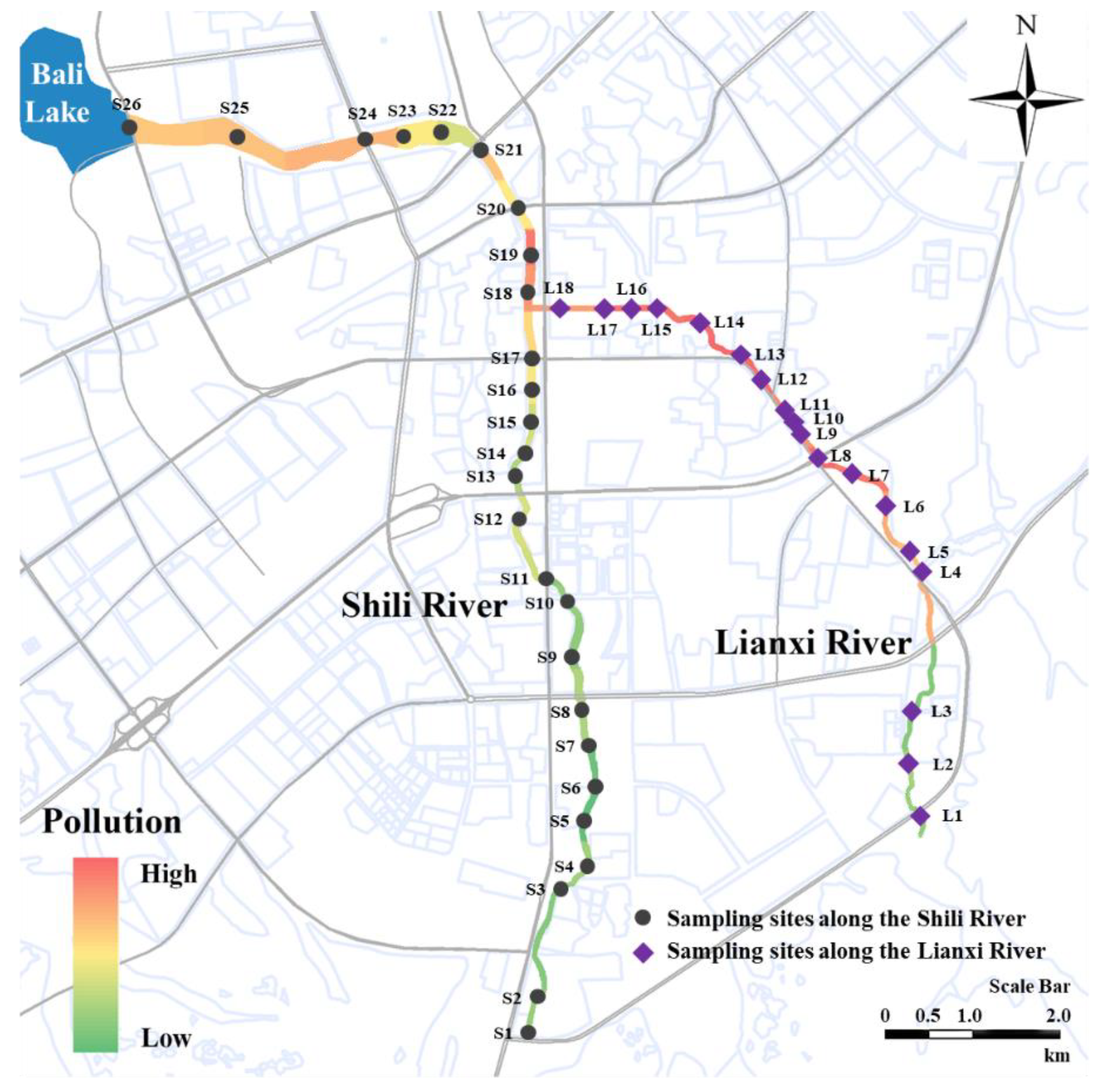
2.1. Study Area

The original sampling sites were set along the Shili River and the Lianxi River in Jiujiang City, Jiangxi Province, China (Figure 1). From the watershed of the Lushan Mountain to the estuary of the Bali Lake, the Shili River has a total length of 13.08 km. Additionally, the Lianxi River is the biggest tributary of the Shili River with a length of 9.62 km from the watershed of the Lushan Mountain to the confluence with the Shili River. Originating from the north slope of the Lushan Mountain, these two rivers flow through the central city of Jiujiang and down into the Bali Lake. Through floodgates, the Bali Lake water eventually flows into the Yangtze River, which is a major water source and canal in China [21]. However, due to the defects in the urban drainage system, the Shili River and the Lianxi River have been suffering from the pollution of both the direct discharge and the overflow of urban sewage. Especially, domestic sewage contributes significantly (over 80%) to the pollution of these two rivers, which poses a great threat to the water quality of the Yangtze River. The spatial and temporal distribution of water quality varies remarkably both in the Shili River and the Lianxi River. These properties are similar with many urban rivers globally, which originate from clear water sources and then suffer from the pollution of urban sewage [22,23,24,25,26]. Thus, the Shili River and the Lianxi River can be representatives for the research on the WQM of urban rivers. The sampling sites were determined based on the published guidelines or standards for surface water monitoring [27,28]. Specifically, 26 sampling sites (red dots) were selected along the Shili River and 18 sites (yellow diamonds) were along the Lianxi River considering the hydrological characteristics, the pollution status of the rivers, and the accessibility of the sites.

2.2. Water Sampling and Chemical Analysis

To understand the general spatial distribution of pollution along the two rivers, surface water samples were collected (approximately 0–10 cm from surface) from the two rivers in December 2020. After collection, all water samples were immediately transferred to the lab in Jiujiang. In Jiujiang, the Dujiu Expressway can act as a boundary, which separates the Shili River and the Lianxi River into the northern and southern sections. According to the local regulatory water quality standard, the limit concentrations of NH3-N, TP, and CODCr for the two rivers are listed in Table 1 [29]. Correspondingly, the concentrations of total phosphate (TP, mg/L), ammonia nitrogen (NH3-N, mg/L), and chemical oxygen demand (CODCr, mg/L) were analyzed respectively using the molybdenum blue method, the Nessler’s reagent spectrophotometry method, and the dichromate method as reported previously [30,31,32]. The detection limits for these parameters are, respectively, 0.01 mg/L, 0.025 mg/L, and 4 mg/L according to administrative standards or previous publications [33,34,35,36]. The difference between the monitoring results of the Shili River and the Lianxi River was analyzed using t-test (Levene’s test for equality of variances) and Nonparametric test after the normality test (Kolmogorov-Smirnov test).

2.3. Monitoring Objects

In the study of monitoring objects, various data-processing methods have been applied to analyze the water quality of these two rivers. The water quality of each sampling sites was assessed using four different methods, namely the single factor (SF) assessment method, the comprehensive pollution index (CPI) including mean pollution index (MPI) and Nemerow pollution index (NPI), the water quality identification index (WQII), and the water quality level index (WQLI) method. The threshold values for the pollution category of each index are listed in Table 2 as previous publications [37,38,39,40].

2.3.1. Single Factor (SF)

The SF assessment method was based on the comparison result of the measured value with the standard value. Generally, the latter value is established according to the regional environmental quality standards for surface water according to previous publications [37]. SF is given by:
SF = C ( i ) C ( 0 )
where C ( i ) and C ( 0 ) respectively represent the measured value and the standard value of the index i.

2.3.2. Comprehensive Pollution Index (CPI)

CPI can be used to comprehensively assess the water quality by calculating the arithmetic mean or weighted mean of the SF. Generally, the CPI can be divided as mean pollution index (MPI) and Nemerow pollution index (NPI). MPI is given by:
MPI = 1 n · i = 1 n SF ( i )
where n represents the number of indexes being assessed.
NPI can highlight the maximum value while illustrating the average and maximum value of the SF [38]. NPI is given by:
NPI = MPI 2   +   SF ( max ) 2 2
where SF ( max ) represents the maximum value among all SF.

2.3.3. Water Quality Identification Index (WQII)

WQII can be used to assess the water quality at different sampling sites and to illustrate the level and data of the water quality, as well as the matching extent with the water functional zones [39]. Accordingly, the surface waters were divided into five water quality levels based on the environmental functions and protection goals. WQII is given by:
WQII = X ( 1 ) . X ( 2 ) X ( 3 )
where for each index, X ( 1 ) is the water quality level, X ( 2 ) is the location of the measured result in the interval of the water quality level, and X ( 3 ) is the comparing result of the water quality level and the functional zone.

2.3.4. Water Quality Level Index (WQLI)

WQLI is the function of the water quality and can be used to decide the water quality level and identify the primary pollution factors [40]. For water quality within the range from “Unpolluted” to “Strongly polluted” (according to the environmental quality standards for surface water [37]), WQLI is given by:
WQLI = WQL ( m ) WQL ( m 1 ) ( C ( m , S ) C ( m 1 , S ) ) × ( C ( i ) C ( m 1 , S ) )   +   WQL ( m 1 )
where C ( i ) represents the measured value of index i, m represents the water quality level of index i, m 1 represents the previous one water quality level of index i, WQL is the corresponding water quality level, and C ( m , S ) and C ( m 1 , S ) are the limit concentrations of the corresponding water level.
For the water quality being “Extremely polluted”, WQLI is given by:
WQLI = 1 / C ( F ) . ( C ( i ) C ( S ) )   +   5
where C ( S ) is the limit concentration of the “strongly polluted” water level, C ( F ) is the limit concentration of the water quality level as listed in Table 1, and the other variables represent the same meanings as before.

2.3.5. Analytical Hierarchy Process (AHP)

The method of AHP analysis of water quality assessment indexes was applied to comprehensively analyze the pollution of 44 sampling sites as published previously [41]. For the local government, NH3-N is regarded as the most concerning pollution index for the Shili River and the Lianxi River, and the judgement criteria of AHP were therefore decided to identify the indexes that can reveal the limit exceeding extent of NH3-N. A total of 11 indexes were analyzed, including using TP, NH3-N, and Chemical Oxygen Demand determined using dichromate method (CODCr) as SF assessment parameters (i.e., SF-TP, SF-NH3, and SF-CODCr), MPI, NPI, using TP, NH3-N, and CODCr as WQII assessment parameters (i.e., WQII-TP, WQII-NH3, WQII-CODCr), using TP, NH3-N, and CODCr as WQLI assessment parameters (i.e., WQLI-TP, WQLI-NH3, WQLI-CODCr). A group of catchment management specialists helped us to decide the importance of each index according to the criteria. The AHP judgement matrix of 11 indexes was decided following the multi-criteria decision aid (MCDA) techniques developed by T.L. Satty [42]. Then, the weight of all indexes was calculated. Specifically, the maximum eigenvalue of the above judgment matrix was firstly calculated. Then, the eigenvectors corresponding to the maximum eigenvalue were obtained and normalized with the formation of the sum of all eigenvectors. Next, the weights of all indexes were calculated using the ratios of each eigenvector to the sum. At last, the consistency of matrix (CR) was examined until it was < 0.1, confirming the rationality of the weights. With the results of AHP, the comprehensive pollution scores of 44 sampling sites were calculated.

2.4. Monitoring Parameters

Statistical methods including correlation analysis, PCA, and cluster analysis were applied to filter out the substitutable parameters. Among all 44 sampling sites, two sampling sites, i.e., S23 and S26 along the Shili River, are within the long-term WQM program of the local government. Based on this, we collected the WQM reports of the S23 and S26 published by the local government from January 2020 to March 2021 [43]. In these reports, the concentrations of Transparency, pH, DO, CODCr, NH3-N, TP, TN, Cu, and oxidation reduction potential (ORP) were available for further analysis. As listed in the reports, the concentration of Cu was analyzed using ICP-MS (300X, NexIon, PerkinElmer, MA, USA, USA). In detail, the monitoring data of these two sampling sites were used to perform Pearson correlation analysis, PCA, and cluster analysis using SPSS 23. Before PCA, the Kaiser-Meyer-Olkin (KMO) measure and Bartlett’s test were applied in advance. The KMO coefficient was 0.637 and the significance of Bartlett’s test of sphericity was 0.000, indicating these data were qualified for PCA. The cluster analysis was calculated using the Pearson relative distance for average linkage between groups.

2.5. Monitoring Frequency

For predicting unknown processes with poor acknowledgement of relation between the input and output, decision tree, especially Random Forest, has been regarded as the most used algorithm [44]. Therefore, Random Forest was used to investigate the correlation among pollutant concentrations after and before precipitation, as well as rainfall depth herein. Sampling site S26 along the Shili River was selected as the assessment section by the local government, which makes the temporal variation of the water quality at this site sensitive as well. Accordingly, long-term water quality monitoring programs were carried out at this site by us. Therefore, sampling site S26 was selected as the monitoring object to study the appropriate monitoring frequency. We collected the WQM results at sampling site S26 before and after precipitation, as well as the rainfall depth data from September 2020 to July 2021. The storm types in the collected precipitation data of Jiujiang were divided into light rain (<10 mm), moderate rain (10–25 mm), and heavy rain (>25 mm) based on the rainfall. The water quality data of sampling site S26 before and after precipitation were used as the representative object. After setting up the databases of the amount of rainfall depth and water quality before and after the precipitation, Random Forest was applied to explore the relationship among the three before-mentioned variables [45]. Briefly, the input data referred to the rainfall depth and the pollutant concentrations before and after precipitation (122 groups for NH3-N model and CODCr model, respectively) and the output data referred to the generated model coefficients for NH3-N and CODCr, respectively. All the input datasets were randomly divided into two parts, i.e., 80% for training and 20% for validation in Random Forest models. Afterwards, the simulated data about pollutant concentrations after precipitation from the models were compared with the practically monitored data. The correlation coefficients between these two datasets were calculated to further validate the accuracy of the constructed models.

3. Results and Discussion

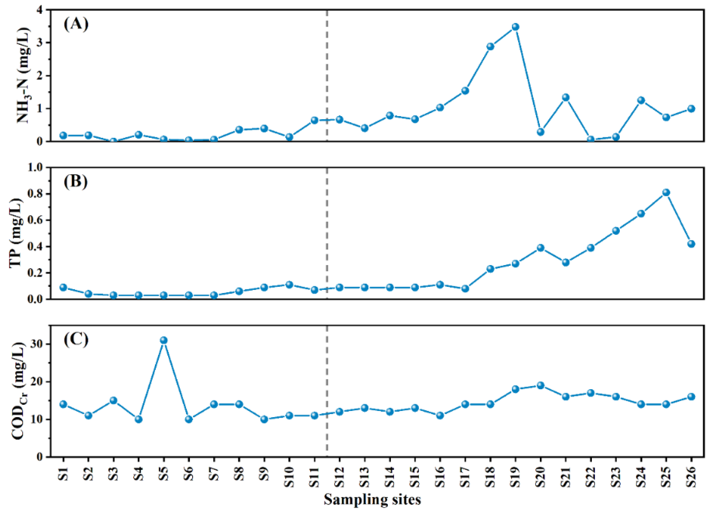
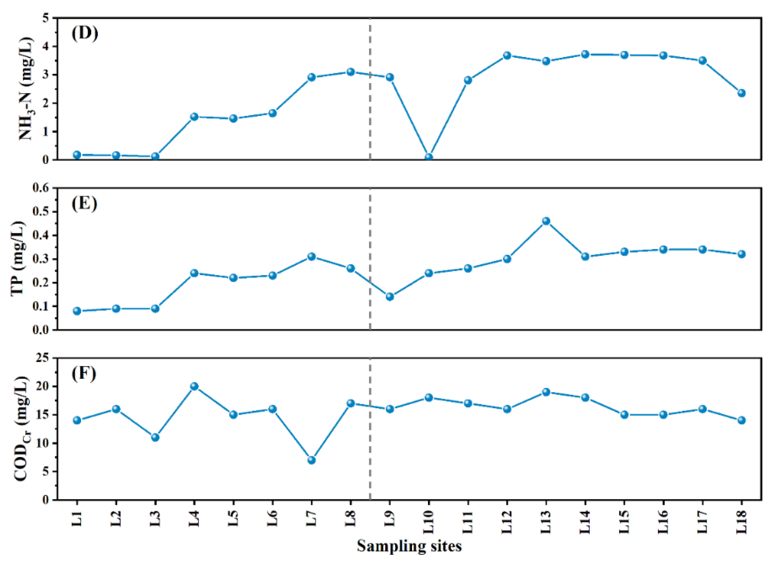
3.1. Distribution of Pollutants in the Shili River and the Lianxi River

The distribution of NH3-N, TP, and CODCr content at sampling sites along the pathway of the Shili River and the Lianxi River is illustrated in Figure 2A–F. As shown in Figure 2A,D, the average concentration of NH3-N in the Lianxi River (2.28 ± 1.35 mg/L) was significantly (p < 0.001) higher than that of the Shili River (0.66 ± 0.82 mg/L). Based on Table 1, the concentrations of sampling sites S18, S19, L4, L6–L9, and L11–L18 were above the limit. Moreover, taking the Dujiu Expressway as the boundary (Figure 1 and the gray dashed lines in Figure 2), the NH3-N concentrations in the northern section of the Shili River and the Lianxi River (1.11 ± 0.95 mg/L and 2.99 ± 1.07 mg/L) were significantly (p < 0.01 and p < 0.05) higher than those in the southern sections (0.21 ± 0.22 mg/L and 1.39 ± 1.11 mg/L). It is well acknowledged that NH3-N is an effective marker for domestic sewage [46,47]. Possibly, the significant difference in NH3-N distribution of the northern and southern sections might be related to the different sewage discharge routes. With the attempt to explain this phenomenon, we investigated the drainage network system of the Shili River and the Lianxi River catchment area. It turns out that the drainage system in the northern section related catchment is generally featured as a combined sewage system, while the system in the southern section is usually separate. It has been reported that, compared with the combined sewage system, the separated sewage system would significantly reduce water pollution discharged to rivers [25,48]. Thus, the severer pollution induced by the combined sewage system reported in these previous works might help explain the higher NH3-N pollution concentrations in the northern sections of the Shili River and the Lianxi River observed in this work.
As regards the TP content illustrated in Figure 2B,E, TP pollution in the Lianxi River (0.25 ± 0.10 mg/L) was a little heavier than that in the Shili River (0.19 ± 0.20 mg/L). According to the C ( F ) for TP (Table 1), the concentrations of sampling sites S20, S22–S26, L7, and L13–L18 were above the C ( F ) , indicating the existence of phosphorus pollution and higher possibilities of eutrophication [49]. Correspondingly, the TP concentrations in the northern section of the Shili River (0.31 ± 0.22 mg/L) and the Lianxi River (0.30 ± 0.08 mg/L) were significantly (p < 0.001 and p < 0.05) higher than those in the southern section (0.05 ± 0.03 mg/L and 0.19 ± 0.08 mg/L). The distribution of TP content was consistent with that of NH3-N content, which further confirms the potential influence of the difference in sewage system between the northern and southern sections. Moreover, there was a remarkable increase of NH3-N and TP content from sampling sites of S17 to S19 along the Shili River. Considering the higher content of pollutants in the Lianxi River as shown in Figure 2D,E, the increase in the Shili River might also be related to the imported pollution from the Lianxi River.
As shown in Figure 2C,F, the distribution of CODCr displayed different trends for the Shili River and the Lianxi River. In general, the average concentration of the Lianxi River (16 ± 3 mg/L) was not significantly different from that of the Shili River (14 ± 4 mg/L). Among 44 sampling sites, almost no sampling site exceeded the C ( F ) listed in Table 1, and only the concentration of sampling site S5 was above C ( F ) . Additionally, no significant difference was discovered between the southern and northern sections. These results suggest that organic pollution reflected by CODCr content is slight and indiscriminate. Only a few sampling sites were marked as polluted, which might be related to individual discharge or unpredicted incidents and requires further research.
Generally, according to the above WQM results, the spatial distribution of the three pollutants varied significantly both in the Shili River and the Lianxi River. Especially, the average NH3-N concentration in the Lianxi River was 3.5 times of that in the Shili River. Moreover, the NH3-N occurrence in the northern sections was much higher than that in the southern sections, i.e., 5.3 times and 2.2 times for the Shili River and the Lianxi River, respectively. Thus, it is of great need to further study the sampling sites geographically, which can help determine the possible pollution sources. Additionally, the C ( F ) exceeding the extent of the three parameters were different from each other, which makes it useful to investigate the monitoring parameters for the identification of pollution and its possible sources. Still, WQM of only one time is not adequate to represent the long-term variation of pollution. Therefore, the appropriate monitoring frequency can help reflect the variation of water quality maximally within limited times.

3.2. Results of Monitoring Objects

The determination of sampling sites is the basic and initial step for the WQM procedure. Water quality assessment results of 44 sampling sites using indexes SF (SF-TP, SF-NH3, and SF-CODCr), MPI, NPI, WQII (WQII-TP, WQII-NH3, and, WQII-CODCr), and WQLI (WQLI-TP, WQLI-NH3, and WQLI-CODCr) are listed in Table S1 in Supplementary Information (SI). Additionally, the water quality assessment index category of each sampling site is listed in Table 3. As shown in Table 3, the water quality of the sampling sites can be divided into six categories. It can be seen that the water quality results of the sampling sites using different methods are inconsistent, which is similar to previous studies about other water systems [50,51]. The AHP method has been regarded as an effective approach for decision making with complicated indexes, which is useful for water quality assessment [17]. Therefore, we applied the method of AHP to comprehensively assess the water quality of every sampling site. According to the criteria of AHP, SF-NH3-N, WQLI-NH3-N, WQII-NH3-N, and MPI were selected as most significant indexes, which could mostly fit the demand of emphasizing the pollution of NH3-N. The judgement matrix is listed in Table S2 (SI), whose consistency is determined as qualified (CR < 0.1). The calculated weights of all 11 indexes are listed in Table S3 (SI).
In a previous study, the researchers adopted the AHP method to evaluate the general pollution extent of the groundwater and determined the most polluted region in a Vietnamese province [52]. Similarly, in this work, according to the weight of all 11 indexes, the comprehensive pollution scores of each sampling site were calculated using the AHP method and the pollution levels of each section in the two rivers are illustrated in Figure 3. With the pollution scores increasing, the illustrated color of two rivers in the figure changes from green to yellow, and finally to red. As shown in Figure 3, there was a remarkable increase of the comprehensive pollution scores from sampling sites of S7 to S8 (by 84%), S15 to S19 (by 181%), and S22 to S24 (by 93%) along the Shili River and L3 to L4 (by 256%), L5 to L8 (by 62%), and L10 to L11 (by 186%) along the Lianxi River. For the investigation of the NH3-N pollution and the possible pollution sources, these sections should be given more attention. On the other hand, no significant variations were observed from sampling sites of S1 to S7 (average variation being 0.7%) and L1 to L3 (average variation being –4%) and the pollution scores remained low in these sections. Therefore, sampling sites in these sections could be cut down.
In general, with the combination of different water quality indexes and the method of AHP, pollution of the concerning pollutants can be emphasized using the comprehensive pollution scores of all sampling sites. Then, for the investigation of the possible pollution sources, sections with sharp decreases in water quality should be given more attention and more sampling sites are needed to be set along these sections. For river sections with little variation in the comprehensive pollution scores and for which the water quality remains satisfying, less WQM effort is needed. By optimizing the sampling sites, the WQM object could be more focused, which makes it possible to detect the crucial monitoring areas more cost-effectively.

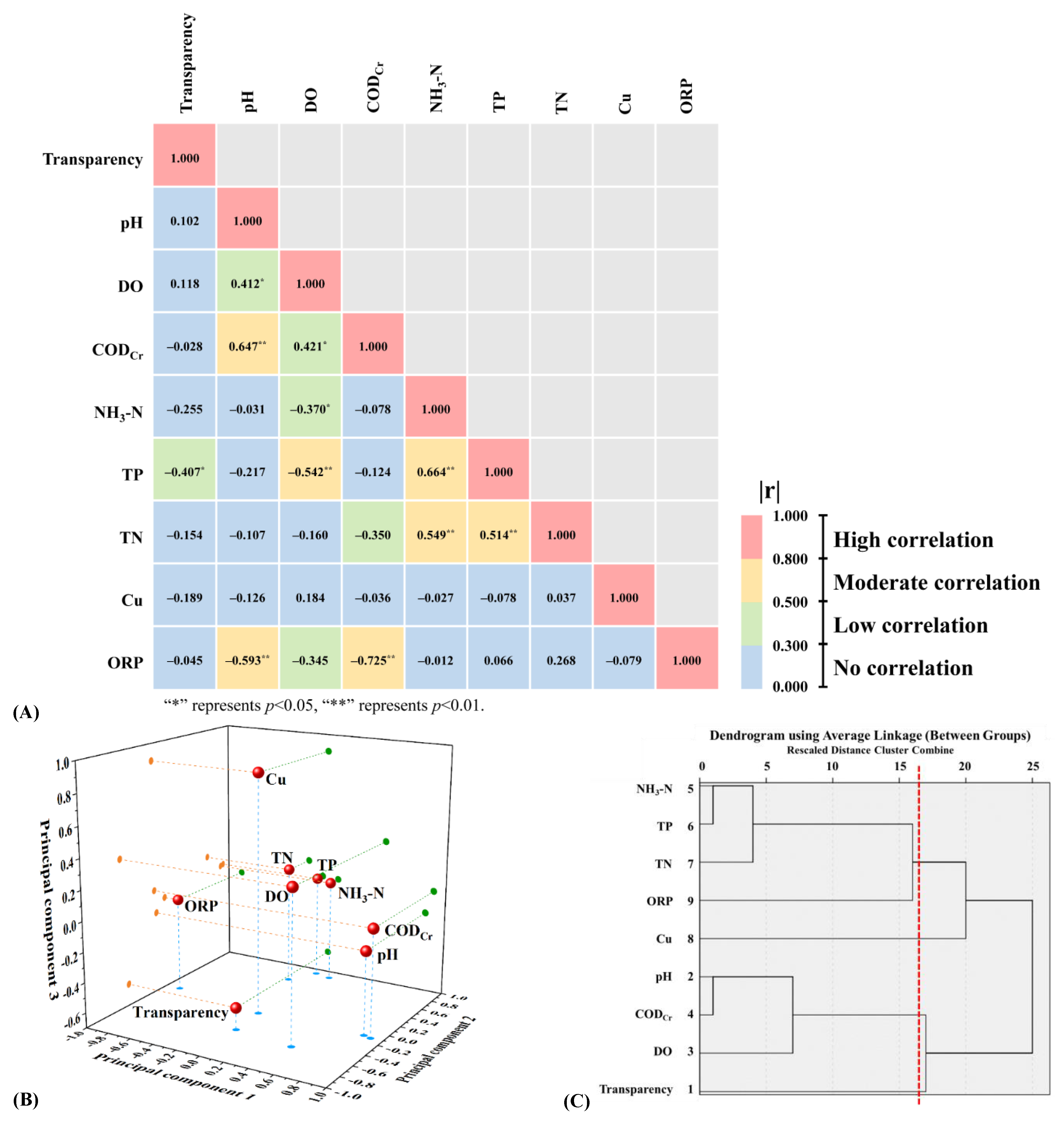
3.3. Results of Monitoring Parameters

Usually, for WQM, the monitoring parameters are large in quantity and complex in relationship. As a result, the accurate selection of monitoring parameters is crucial to increasing monitoring efficiency. Statistical relationships among different parameters could help identify the substitutable parameters for monitoring. As mentioned above, sampling sites S23 and S26 were chosen for the investigation of monitoring parameters due to the availability of multi-parameter WQM data from the local government. Statistical methods of correlation analysis, PCA, and cluster analysis were applied to identify the optimal parameters for WQM.
Pearson correlation coefficients between Transparency, pH, DO, CODCr, NH3-N, TP, TN, Cu, and ORP were calculated and illustrated in Figure 4A. Obviously, strong and significant correlations (p < 0.01) existed among parameters of CODCr, pH, and ORP, as well as among TP, DO, NH3-N, and TN, all with Pearson correlation coefficients exceeding 0.5. It is well admitted that the parameters with strong correlations can indicate similar pollution sources as reported previously [53,54,55]. For instance, a published work observed a strong correlation between TP and total organic carbon in a German river, which probably indicates the same pathway and source for these two pollutants [53]. Accordingly, the above-mentioned parameters with strong and significant correlations might come from the same situation. Other parameters without strong and significant correlations like Cu might come from some different sources.
Furthermore, the PCA was carried out to help reveal the relationships among various indexes. According to the PCA result with varimax rotated solution as shown in Figure 4B, there were a total of three principal components (total 70.047%, 34.861%, 21.697%, and 13.490% for Principal Components 1, 2, and 3, respectively) among all parameters. Generally, the results of PCA were consistent with those of correlation analysis. Principal component 1 was strongly correlated with pH, CODCr, and ORP. Meanwhile, significant correlations were observed among these three parameters. This suggests that these three parameters might have similar pollution sources, like waste water from the food industry or fiber glass plants as published previously [56]. Principal component 2 was strongly correlated with DO, NH3-N, TP, and TN, and these four parameters were significantly correlated with each other. It has been reported that typical domestic waste water is usually polluted with NH3-N, TP, and TN, and sometimes lacks oxygen [57]. This suggests that the parameters correlated with principal component 2 might originate from domestic waste water. Principal component 3 is strongly correlated with Transparency and Cu, also indicating their potentially different pollution sources as mentioned in the correlation analysis. Cu is speculated be related to certain industries and the incentive of Transparency is uncertain and requires further exploration.
As a useful tool, the cluster analysis has been applied in the identification of main pollution patterns among various and complex pollutant mixtures [58]. In that case, three major pollution patterns were determined with the assistance of the cluster analysis in a Chinese river, i.e., from wastewater treatment plants, from the confluence with other rivers, and from diffuse and random inputs. In our work, the cluster analysis of nine parameters was also carried out and the results are shown in Figure 4C. After comprehensively considering the statistical analysis results above-mentioned and the local pollution conditions, the nine parameters could be divided into four groups with the distance of ~17 (the red dashed line in Figure 4C) after the cluster analysis. The four groups were composed of group 1 (NH3-N, TP, TN, and ORP), group 2 (Cu), group 3 (pH, CODCr, and DO), and group 4 (Transparency).
Based on the above multiple statistical analyses, the results from the three analyses generally displayed satisfactory consistency. Combining these analytical results about the chosen representative sites, we could come up with some suggestive conclusions and speculations. For the water quality of the Shili River and the Lianxi River, parameters of NH3-N, TP, and TN could be classified as one group to represent domestic waste water pollution; parameters of CODCr and pH could be classified as one group to represent light industry waste water pollution; and the parameter of Cu could be classified as one group to represent heavy industry waste water pollution. For Transparency, its incentive might be varied and complicated, and more efforts should be made to elucidate the potential sources in future.
Therefore, the research about the monitoring parameters based on the representative sampling sites is of significance to future urban WQM. With the statistical methods like correlation analysis, PCA, and cluster analysis, etc., various parameters can be classified into a few groups. Furthermore, these groups can be optimized according to the possible pollution sources of the target rivers. Usually, parameters in the same group can be regarded as alternative parameters for each other. Under some conditions, such as when manpower and material resources are limited or the operation is inconvenient, certain parameters from each group can be used as the representative indicators for WQM. This can improve the efficiency of monitoring under the basic assurance of monitoring accuracy, which is important for the fair arrangement of resources in WQM.

3.4. Results of Monitoring Frequency

Monitoring frequency is of significance to the effective detection of pollution, especially in view of precipitation. It has been reported that the precipitation would have a remarkable impact on the water quality of urban rivers [59,60,61]. Thus, the appropriate monitoring frequency, especially like the conditions before and after precipitation, can contribute to the reasonable allocation of WQM programs.
After analyzing the water quality data of sampling site S26 before and after precipitation, the correlation between the concentrations of pollutants (NH3-N and CODCr) after precipitation and rainfall depth are illustrated in Figure 5. As shown in Figure 5A, the concentrations of NH3-N barely changed with the increase of rainfall depth in the storm type of light rain. With the storm type increasing to moderate rain, the NH3-N concentrations increased remarkably with the increase of rainfall depth (Figure 5B). Furthermore, the NH3-N concentrations decreased remarkably with the increase of rainfall depth in the storm type of heavy rain (Figure 5C). Similarly, as illustrated in Figure 5D–F, the concentrations of CODCr also displayed the trend of being nearly unchanging, increasing, and decreasing with the storm type changing from light to moderate, and to heavy. The consistent changing trends of NH3-N and CODCr concentrations can well reflect the influence of precipitation on pollutions, which is basically consistent with the published results [62,63,64]. It has been reported that large quantities of land surface pollutants can be transported into rivers by storm runoff [62]. Moreover, combined sewer overflows have been a threatening potential pollution source for urban water environments [63]. During the storm type of light rain, it is more likely that no significant runoff would take place and the interception measures in the sewer system would perform well as published previously [64]. Accordingly, the concentrations of pollutants show no significant change during light rain depth. Then, with the increase of rainfall depth, the land surface pollutant concentrations and the intensity to the interception system would rise gradually, which was also mentioned in the previous publication [65]. This may help explain the significant increase of pollutant concentrations with the increase of rainfall depth in the storm type of moderate rain observed in this work. Eventually, with the storm type increased to heavy rain, the pollution in the rivers might have been diluted by rain storms, which could help explain the decrease of pollutant concentrations with the increase of rainfall depth in the storm type of heavy rain (Figure 5C,F). The observed dilution effects of heavy rain on pollution were also in accordance with the previous publication [59]. Therefore, at the stages with sharp variations in pollutant concentration, like the NH3-N during the storm type of moderate and heavy as well as the CODCr during the heavy storm type, more attention should be paid during such periods. For Jiujiang City, the heavy storm type usually appears in late spring to early summer and, possibly, more WQM programs (i.e., higher sampling frequency) should be adopted to realize efficient monitoring.
The accurate prediction with modelling based on the existing data is a useful and convenient solution for efficient WQM, which is also a key means of smart water systems [66]. Therefore, a water quality-predicting model after precipitation was explored herein for effective monitoring as well as further possible applications in smart water systems. The model refers to the relation among the water quality and the rain depth fitted using the machine learning algorithm of Random Forest. By analyzing the pollutant concentrations before and after precipitation under different precipitation conditions, it was found that the pollutant concentration after precipitation showed a trend of increasing firstly and decreasing afterwards. This can be fitted by a quadratic function that monotonically increases and then decreases. The fitting results are displayed in Equations (7) and (8) for NH3-N and CODCr, respectively. Then, the fitting performance was evaluated through comparing the simulation results with the monitored results. As illustrated in Figure 6, the simulation results were quite consistent with the monitored values, showing good linear relationship with the Pearson correlation coefficients being 0.89 and 0.97 correspondingly, indicating the satisfactory accuracy and persuasive power of the established models. In published research, the predicted data of multiple pollutants (like COD and TP) have been generated with the Random Forest algorithm, which also showed satisfactory linearities with the observed data [19]. These results suggest the huge potential of Random Forest in predicting pollution, especially with poor knowledge of input and output relationships. Herein, based on the predicted data from Random Forest and the subsequent fitting models, the pollutant concentration after precipitation could be calculated using the concentration of pollutants before precipitation and the rainfall depth.
C NH 3 - N ,   after = C NH 3 - N ,   before ( 0 . 00179 rainfall 2 + 0 . 16178 rainfall + 0 . 03088 )
C COD Cr ,   after = C COD Cr ,   before ( 0 . 00337 rainfall 2 + 0 . 30619 rainfall 0 . 65692 )
where, C NH 3 - N ,   after and C COD Cr ,   after respectively represents the concentration of NH3-N and CODCr after precipitation, C NH 3 - N ,   before and C COD Cr ,   before respectively represents the concentration of NH3-N and CODCr before precipitation, and rainfall represents the rainfall depth.
In general, for the WQM frequency, it is suggested to firstly collect the long-term data of precipitation and water quality before precipitation at one representative sampling site. Using the fitting model, water quality after precipitation could be predicted. Based on both the measured and simulated water quality data, the periodic variation of water quality could be well estimated, e.g., the annual variation of the concentration of pollutants during the storm types of light, moderate, or heavy. Then, the WQM frequency could be designed according to the variation of water quality, which helps reflect the future water quality fluctuation to the furthest extent within limited times. Specifically, more WQM programs should be carried out during the period of large variation of water quality. The optimized WQM frequency is, consequently, of significance to the detection of pollution and even to the tracing of the pollution source. In addition, the construction of the water quality predicting model is also of significance for the development of smart water systems.

4. Conclusions

The current work was carried out to multi-dimensionally investigate and comprehensively analyze the water quality of two representative urban rivers. Generally, the distribution of the NH3-N, TP, and CODCr fluctuated significantly in both rivers. The assessment of water quality at 44 sampling sites with the AHP method can help optimize the monitoring object with the emphasis on the sections with a dramatic decrease of water quality. The substitutional relationship among different monitoring parameters was achieved through correlation analysis, principal component analysis, and cluster analysis, which can help determine the optimal monitoring parameters. Relationships among concentrations of pollutants after precipitation, rainfall depth, and concentrations before precipitation were constructed using statistical methods and machine learning algorithms. On this basis, sampling frequency could be optimized with the prediction of pollutant concentrations after precipitation, and more sampling programs should be carried out during the period of large variations in water quality. In a word, this work can suggest an innovative and multi-dimensional solution for water quality investigation and assessment as well as the optimization of the existing WQM strategy, which is of significance to realize efficient water quality monitoring, sustainable water source management, and smart water system construction in urban water environments.

Supplementary Materials

The following supporting information can be downloaded at: https://www.mdpi.com/article/10.3390/su14074174/s1, Table S1: Water quality assessment results of different sampling sites using five indexes; Table S2: Judgement matrix of 11 water quality assessment indexes; Table S3: Weight of 11 water quality assessment indexes; Table S4: Range with the permissible values of three parameters at 44 sampling sites along the two rivers during the sampling campaign on December, 2020; Table S5: Range with the permissible values of four parameters at sampling sites S23 and S26 along the Shili river from January 2020 to March 2021.

Author Contributions

Conceptualization, methodology, investigation, writing—original draft preparation, X.J.; project administration, funding acquisition, J.C.; supervision, writing—review and editing, Y.G. All authors have read and agreed to the published version of the manuscript.

Funding

This research was funded by the Research Project of China Three Gorges Corporation (Research on Key Technology of Urban Water Environment Monitoring System and Pollution Traceability), grant number [202003134].

Institutional Review Board Statement

Not applicable.

Informed Consent Statement

Not applicable.

Data Availability Statement

Not applicable.

Acknowledgments

We thank Jin Wei and Hang Yang for their support in this work. We thank the anonymous reviewers, editor for their constructive comments on the manuscript.

Conflicts of Interest

The authors declare no conflict of interest.

References

  1. Hobbie, S.E.; Finlay, J.C.; Janke, B.D.; Nidzgorski, D.A.; Millet, D.B.; Baker, L.A. Contrasting nitrogen and phosphorus budgets in urban watersheds and implications for managing urban water pollution. Proc. Nat. Acad. Sci. USA 2017, 114, 4177–4182. [Google Scholar] [CrossRef] [PubMed] [Green Version]
  2. Puckett, L.J. Identifying the major sources of nutrient water pollution. Environ. Sci. Technol. 1995, 29, 408A–414A. [Google Scholar] [CrossRef]
  3. Xia, J.; Zhang, Y.; Xiong, L.; He, S.; Wang, L.; Yu, Z. Opportunities and challenges of the Sponge City construction related to urban water issues in China. Sci. China Earth Sci. 2017, 60, 652–658. [Google Scholar] [CrossRef]
  4. Wang, H.; Wu, M.; Deng, Y.; Tang, C.; Yang, R. Surface water quality monitoring site optimization for Poyang Lake, the largest freshwater lake in China. Int. J. Environ. Res. Public Health 2014, 11, 11833–11845. [Google Scholar] [CrossRef] [PubMed] [Green Version]
  5. Mantzafleri, N.; Psilovikos, A.; Blanta, A. Water quality monitoring and modeling in Lake Kastoria, using GIS. Assessment and management of pollution sources. Water Resour. Manage. 2009, 23, 3221–3254. [Google Scholar] [CrossRef]
  6. Ahuja, S. Monitoring Water Quality: Pollution Assessment, Analysis, and Remediation; Elsevier: Amsterdam, The Netherlands, 2013. [Google Scholar]
  7. Guzinski, R.; Kass, S.; Huber, S.; Bauer-Gottwein, P.; Jensen, I.H.; Naeimi, V.; Doubkova, M.; Walli, A.; Tottrup, C. Enabling the use of earth observation data for integrated water resource management in Africa with the water observation and information system. Remote Sens. 2014, 6, 7819–7839. [Google Scholar] [CrossRef] [Green Version]
  8. Yu, W.; Ma, L. External government performance evaluation in China: Evaluating the evaluations. Public Perform. Manage. 2015, 39, 144–171. [Google Scholar] [CrossRef]
  9. Canter, L.W. River Water Quality Monitoring; CRC Press: Boca Raton, FL, USA, 1985. [Google Scholar]
  10. Bartram, J.; Ballance, R. Water Quality Monitoring: A Practical Guide to the Design and Implementation of Freshwater Quality Studies and Monitoring Programmes; CRC Press: Boca Raton, FL, USA, 1996. [Google Scholar]
  11. Gray, N. Water technology: An introduction for environmental scientists and engineers, 3rd ed.; Taylor & Francis: Oxford, UK, 2010. [Google Scholar]
  12. Dong, J.; Wang, G.; Yan, H.; Xu, J.; Zhang, X. A survey of smart water quality monitoring system. Environ. Sci. Pollut. Res. 2015, 22, 4893–4906. [Google Scholar] [CrossRef]
  13. Behmel, S.; Damour, M.; Ludwig, R.; Rodriguez, M.J. Water quality monitoring strategies—a review and future perspectives. Sci. Total Environ. 2016, 571, 1312–1329. [Google Scholar] [CrossRef] [PubMed]
  14. Geological Survey (US); Office of Water Data Coordination. National Handbook of Recommended Methods for Water-Data Acquisition; US Government Printing Office: Reston, VA, USA, 1977.
  15. Ouyang, Y. Evaluation of river water quality monitoring stations by principal component analysis. Water Res. 2005, 39, 2621–2635. [Google Scholar] [CrossRef]
  16. Khalil, B.; Ouarda, T.B.M.J.; St-Hilaire, A.; Chebana, F. A statistical approach for the rationalization of water quality indicators in surface water quality monitoring networks. J. Hydrol. 2010, 386, 173–185. [Google Scholar] [CrossRef]
  17. Karamouz, M.; Kerachian, R.; Akhbari, M.; Hafez, B. Design of river water quality monitoring networks: A case study. Environ. Model Assess. 2008, 14, 705. [Google Scholar] [CrossRef]
  18. Chen, K.; Chen, H.; Zhou, C.; Huang, Y.; Qi, X.; Shen, R.; Liu, F.; Zuo, M.; Zou, X.; Wang, J.; et al. Comparative analysis of surface water quality prediction performance and identification of key water parameters using different machine learning models based on big data. Water Res. 2020, 171, 115454. [Google Scholar] [CrossRef] [PubMed]
  19. Jeung, M.; Baek, S.; Beom, J.; Cho, K.H.; Her, Y.; Yoon, K. Evaluation of random forest and regression tree methods for estimation of mass first flush ratio in urban catchments. J. Hydrol. 2019, 575, 1099–1110. [Google Scholar] [CrossRef]
  20. Wang, F.; Wang, Y.; Zhang, K.; Hu, M.; Weng, Q.; Zhang, H. Spatial heterogeneity modeling of water quality based on random forest regression and model interpretation. Environ. Res. 2021, 202, 111660. [Google Scholar] [CrossRef] [PubMed]
  21. Qiu, J. Yangtze finless porpoises in peril. Nature 2012. [Google Scholar] [CrossRef]
  22. Yang, W.; Zhao, Y.; Wang, D.; Wu, H.; Lin, A.; He, L. Using principal components analysis and IDW interpolation to determine spatial and temporal changes of surface water quality of Xin’anjiang River in Huangshan, China. Int. J. Environ. Res. Public Health 2020, 17, 2942. [Google Scholar] [CrossRef] [PubMed]
  23. Xu, Z.; Xu, J.; Yin, H.; Jin, W.; Li, H.; He, Z. Urban river pollution control in developing countries. Nat. Sustain. 2019, 2, 158–160. [Google Scholar] [CrossRef]
  24. Vásquez, C.; Calva, J.; Morocho, R.; Donoso, D.A.; Benítez, Á. Bryophyte communities along a tropical urban river respond to heavy metal and arsenic pollution. Water 2019, 11, 813. [Google Scholar] [CrossRef] [Green Version]
  25. Ouattara, N.K.; Garcia-Armisen, T.; Anzil, A.; Brion, N.; Servais, P. Impact of wastewater release on the faecal contamination of a small urban river: The Zenne River in Brussels (Belgium). Water Air Soil. Pollut. 2014, 225, 2043. [Google Scholar] [CrossRef]
  26. Riechel, M.; Matzinger, A.; Pawlowsky-Reusing, E.; Sonnenberg, H.; Uldack, M.; Heinzmann, B.; Caradot, N.; Seggern, D. Impacts of combined sewer overflows on a large urban river–understanding the effect of different management strategies. Water Res. 2016, 105, 264–273. [Google Scholar] [CrossRef] [PubMed]
  27. Ministry of Ecology and Environment of the People’s Republic of China. Technical Specifications Requirements for Monitoring of Surface Water and Waste Water (HJ/T 91—2002); China Environmental Science Press: Beijing, China, 2002. (In Chinese)
  28. Ministry of Ecology and Environment of the People’s Republic of China. Methods of Analysis for Water and Wastewater Monitoring, 4th ed.; China Environmental Science Press: Beijing, China, 2002. (In Chinese)
  29. Chinese Government Procurement. The First Phase of the Comprehensive Treatment of the Water Environment System in the Downtown Area of Jiujiang—PPP Project Contract. Available online: http://www.ccgp.gov.cn/cggg/dfgg/qtgg/201901/t20190107_11475588.htm (accessed on 2 March 2022). (In Chinese)
  30. Murphy, J.; Riley, J.P. A modified single solution method for the determination of phosphate in natural waters. Anal. Chim. Acta 1962, 27, 31–36. [Google Scholar] [CrossRef]
  31. Ji, X.; Liu, C.; Pan, G. Interfacial oxygen nanobubbles reduce methylmercury production ability of sediments in eutrophic waters. Ecotox. Environ. Safe. 2020, 188, 109888. [Google Scholar] [CrossRef] [PubMed]
  32. American Public Health Association; American Water Works Association; Water Environment Federation. Standard Methods for the Examination of Water and Wastewater, 20th ed.; Clesceri, L.S., Greenberg, A.E., Eaton, A.D., Eds.; American Public Health Association: Washington, DC, USA, 1999. [Google Scholar]
  33. Ren, J.; Li, N.; Wei, H.; Li, A.; Yang, H. Efficient removal of phosphorus from turbid water using chemical sedimentation by FeCl3 in conjunction with a starch-based flocculant. Water Res. 2020, 170, 115361. [Google Scholar] [CrossRef] [PubMed]
  34. Ministry of Ecology and Environment of the People’s Republic of China. Water Quality—Determination of Total Phosphorus—Ammonium Molybdate Spectrophotometric Method (GB/T 11893—1989); China Environmental Science Press: Beijing, China, 1989. (In Chinese)
  35. Ministry of Ecology and Environment of the People’s Republic of China. Water Quality—Determination of Ammonia Nitrogen—Nessler’s Reagent Spectrophotometry (HJ 535—2009); China Environmental Science Press: Beijing, China, 2009. (In Chinese)
  36. Ministry of Ecology and Environment of the People’s Republic of China. Water Quality—Determination of the Chemical Oxygen Demand—Dichromate Method (HJ 828—2017); China Environmental Science Press: Beijing, China, 2017. (In Chinese)
  37. Ministry of Ecology and Environment of the People’s Republic of China; General Administration of Quality Supervision, Inspection and Quarantine of the People’s Republic of China. Environmental Quality Standards for Surface Water (GB 3838—2002); China Environmental Science Press: Beijing, China, 2002. (In Chinese)
  38. Brady, J.P.; Ayoko, G.A.; Martens, W.N.; Goonetilleke, A. Development of a hybrid pollution index for heavy metals in marine and estuarine sediments. Environ. Monit. Assess. 2015, 187, 306. [Google Scholar] [CrossRef] [PubMed] [Green Version]
  39. Xu, Z. Comprehensive water quality identification index for environmental quality assessment of surface water. J. Tongji Univ. (Nat. Sci.) 2005, 33, 482–488. (In Chinese) [Google Scholar]
  40. Deng, J. Water Quality Level Index (WLI) and its application in water quality assessment and early warning in coastal areas of southern Guangxi. Yangtze River 2021, 52, 18–24. (In Chinese) [Google Scholar]
  41. Karimi, A.R.; Mehrdadi, N.; Hashemian, S.J.; Bidhendi, G.R.N.; Moghaddam, R.T. Selection of wastewater treatment process based on the analytical hierarchy process and fuzzy analytical hierarchy process methods. Int. J. Environ. Sci. Technol. 2011, 8, 267–280. [Google Scholar] [CrossRef] [Green Version]
  42. Saaty, T.L. The Analytic Hierarchy Process; Mcgrew-Hill: New York, NY, USA, 1980. [Google Scholar]
  43. Jiujiang Ecological Environment Bureau. Monitoring Data of Black and Odorous Water Bodies in Urban Built-Up Areas of Jiujiang City. Available online: http://sthjj.jiujiang.gov.cn/zwgk_215/zdly/hjzljc/hjzkgb/ (accessed on 2 March 2022). (In Chinese)
  44. Lu, C.; Xu, Z.; Dong, B.; Zhang, Y.; Wang, M.; Zeng, Y.; Zhang, C. Machine learning for the prediction of heavy metal removal by chitosan-based flocculants. Carbohyd. Polym. 2022, 285, 119240. [Google Scholar] [CrossRef]
  45. Breiman, L. Random Forests. Mach. Learn. 2001, 45, 5–32. [Google Scholar] [CrossRef] [Green Version]
  46. Been, F.; Rossi, L.; Ort, C.; Rudaz, S.; Delémont, O.; Esseiva, P. Population normalization with ammonium in wastewater-based epidemiology: Application to illicit drug monitoring. Environ. Sci. Technol. 2014, 48, 8162–8169. [Google Scholar] [CrossRef] [PubMed]
  47. Zheng, Q.D.; Lin, J.G.; Pei, W.; Guo, M.X.; Wang, Z.; Wang, D.G. Estimating nicotine consumption in eight cities using sewage epidemiology based on ammonia nitrogen equivalent population. Sci. Total Environ. 2017, 590–591, 226–232. [Google Scholar] [CrossRef] [PubMed]
  48. Huang, D.; Liu, X.; Jiang, S.; Wang, H.; Wang, J.; Zhang, Y. Current state and future perspectives of sewer networks in urban China. Front. Environ. Sci. Eng. 2018, 12, 2. [Google Scholar] [CrossRef]
  49. Jarvie, H.P.; Neal, C.; Withers, P.J.A. Sewage-effluent phosphorus: A greater risk to river eutrophication than agricultural phosphorus? Sci. Total Environ. 2006, 360, 246–253. [Google Scholar] [CrossRef]
  50. Adimalla, N. Application of the Entropy weighted water quality index (EWQI) and the pollution index of groundwater (PIG) to assess groundwater quality for drinking purposes: A case study in a rural area of Telangana State, India. Arch. Environ. Con. Tox. 2021, 80, 31–40. [Google Scholar] [CrossRef] [PubMed]
  51. Yin, H.L.; Xu, Z.X. Comparative study on typical river comprehensive water quality assessment methods. Resour. Environ. Yangtze Basin 2008, 17, 729–733. (In Chinese) [Google Scholar]
  52. Minh, H.V.T.; Avtar, R.; Kumar, P.; Tran, D.Q.; Ty, T.V.; Behera, H.C.; Kurasaki, M. Groundwater quality assessment using fuzzy-AHP in An Giang Province of Vietnam. Geosciences 2019, 9, 330. [Google Scholar] [CrossRef] [Green Version]
  53. Meyer, A.M.; Klein, C.; Fünfrocken, E.; Kautenburger, R.; Beck, H.P. Real-time monitoring of water quality to identify pollution pathways in small and middle scale rivers. Sci. Total Environ. 2019, 651, 2323–2333. [Google Scholar] [CrossRef] [PubMed]
  54. Putri, M.S.A.; Lou, C.H.; Syai’in, M.; Ou, S.H.; Wang, Y.C. Long-term river water quality trends and pollution source apportionment in Taiwan. Water 2018, 10, 1394. [Google Scholar] [CrossRef] [Green Version]
  55. Duan, W.; He, B.; Nover, D.; Yang, G.; Chen, W.; Meng, H.; Zou, S.; Liu, C. Water quality assessment and pollution source identification of the eastern Poyang Lake basin using multivariate statistical methods. Sustainability 2016, 8, 133. [Google Scholar] [CrossRef] [Green Version]
  56. Melchiors, M.S.; Piovesan, M.; Becegato, V.R.; Becegato, V.A.; Tambourgi, E.B.; Paulino, A.T. Treatment of wastewater from the dairy industry using electroflocculation and solid whey recovery. J. Environ. Manage. 2016, 182, 574–580. [Google Scholar] [CrossRef]
  57. Xu, Z.; Wang, L.; Yin, H.; Li, H.; Schwegler, B.R. Source apportionment of non-storm water entries into storm drains using marker species: Modeling approach and verification. Ecol. Indic. 2016, 61, 546–557. [Google Scholar] [CrossRef]
  58. Beckers, L.M.; Brack, W.; Dann, J.P.; Krauss, M.; Müller, E.; Schulze, T. Unraveling longitudinal pollution patterns of organic micropollutants in a river by non-target screening and cluster analysis. Sci. Total Environ. 2020, 727, 138388. [Google Scholar] [CrossRef]
  59. Yang, L.; Li, J.; Zhou, K.; Feng, P.; Dong, L. The effects of surface pollution on urban river water quality under rainfall events in Wuqing district, Tianjin, China. J. Clean. Prod. 2021, 293, 126136. [Google Scholar] [CrossRef]
  60. Xu, Z.; Xiong, L.; Li, H.; Liao, Z.; Yin, H.; Wu, J.; Xu, J.; Chen, H. Influences of rainfall variables and antecedent discharge on urban effluent concentrations and loads in wet weather. Water Sci. Technol. 2017, 75, 1584–1598. [Google Scholar] [CrossRef] [Green Version]
  61. Walsh, C.J.; Roy, A.H.; Feminella, J.W.; Cottingham, P.D.; Groffman, P.M.; Morgan, R.P. The urban stream syndrome: Current knowledge and the search for a cure. J. N. Am. Benthol. Soc. 2005, 24, 706–723. [Google Scholar] [CrossRef]
  62. Hiki, K.; Nakajima, F.; Tobino, T. Causes of highway road dust toxicity to an estuarine amphipod: Evaluating the effects of nicotine. Chemosphere 2017, 168, 1365–1374. [Google Scholar] [CrossRef] [PubMed]
  63. Kay, P.; Hughes, S.R.; Ault, J.R.; Ashcroft, A.E.; Brown, L.E. Widespread, routine occurrence of pharmaceuticals in sewage effluent, combined sewer overflows and receiving waters. Environ. Pollut. 2017, 220, 1447–1455. [Google Scholar] [CrossRef] [Green Version]
  64. Peng, H.Q.; Liu, Y.; Wang, H.W.; Gao, X.L.; Ma, L.M. Event mean concentration and first flush effect from different drainage systems and functional areas during storms. Environ. Sci. Pollut. Res. 2016, 23, 5390–5398. [Google Scholar] [CrossRef]
  65. Li, T.; Tan, Q.; Zhu, S. Characteristics of combined sewer overflows in Shanghai and selection of drainage systems. Water Environ. J. 2010, 24, 74–82. [Google Scholar] [CrossRef]
  66. Liu, P.; Wang, J.; Sangaiah, A.K.; Xie, Y.; Yin, X. Analysis and prediction of water quality using LSTM deep neural networks in IoT environment. Sustainability 2019, 11, 2058. [Google Scholar] [CrossRef] [Green Version]
Figure 1. Sampling sites along the Shili River and the Lianxi River in Jiujiang City, Jiangxi Province, China.
Sustainability 14 04174 g001
Figure 2. Distribution of concentrations of (A) NH3-N, (B) TP, and (C) CODCr in the Shili River and (D) NH3-N, (E) TP, and (F) CODCr in the Lianxi River. The gray dashed line represents the boundary of the northern and southern sections of these two rivers.
Sustainability 14 04174 g002aSustainability 14 04174 g002b
Figure 3. Distribution of comprehensive pollution scores along the Shili River and the Lianxi River.
Sustainability 14 04174 g003
Figure 4. Analytical results of (A) Pearson correlation coefficient, (B) rotated principal component analysis, and (C) cluster analysis among each WQM parameter. The red dashed line represents the distance for cluster analysis.
Sustainability 14 04174 g004
Figure 5. Correlation between NH3-N concentrations with rainfall depths in the storm types of (A) light rain, (B) moderate rain, and (C) heavy rain; CODCr concentrations with rainfall depths in the storm types of (D) light rain, (E) moderate rain, and (F) heavy rain.
Sustainability 14 04174 g005aSustainability 14 04174 g005b
Figure 6. Comparison results of the simulation result and the measured result of concentrations of (A) NH3-N and (B) CODCr.
Sustainability 14 04174 g006
Table 1. Limit concentration of the Shili River and the Lianxi River according to the local regulatory standard [29].
ParameterLimit Concentration (mg/L)
Southern SectionNorthern Section
NH3-N1.52.0
TP0.3
CODCr30
Table 2. The threshold value of each index to represent different water quality categories [37,38,39,40].
Quality of WaterSingle
Factor (SF)
Comprehensive Pollution Index (CPI)Water Quality
Identification Index (WQII)
Water Quality Level Index (WQLI)
Mean Pollution Index (MPI)Nemerow Pollution Index (NPI)
Unpolluted 1 0 . 20 1 1 . 0     X ( 1 ) . X ( 2 )     2 . 0 0     WQLI     1
Slightly polluted > 1 0 . 20   <   MPI     0 . 40 1   <   NPI     2 2 . 0   <   X ( 1 ) . X ( 2 )     3 . 0 1   <   WQLI     2
Moderately polluted 0 . 40   <   MPI     0 . 70 2   <   NPI     3 3 . 0   <   X ( 1 ) . X ( 2 )     4 . 0 2   <   WQLI     3
Polluted 0 . 70   <   MPI     1 . 00 4 . 0   <   X ( 1 ) . X ( 2 )     5 . 0 3   <   WQLI     4
Strongly polluted 1 . 00   <   MPI     2 . 00 3   <   NPI   5 5 . 0   <   X ( 1 ) . X ( 2 )     6 . 0 4   <   WQLI     5
Extremely polluted > 2 . 00 > 5 X ( 1 ) . X ( 2 )   >   6 . 0 WQLI   >   5
Table 3. Water quality assessment index category of different sampling sites using five indexes.
Water QualitySFMPINPIWQIIWQLI
TPNH3-NCODCrTPNH3-NCODCrTPNH3-NCODCr
UnpollutedS1–S19, S21, L1–L6, L8–L12S1–S17, S20–S28, L1–L5, L10S1–S4, S6–S28, L1–L18S3–S4, S6S1–S17, S21, S27–S28, L1–L6, L10S27S3, S5–S7, S10, S22–S23, S27–S28, L2–L3, L10S1–S4, S6–S18, S24–S25, S27–S28, L1, L3, L5, L7, L15, L16, L18S27S3, S5–S7, S10, S22–S23, S27–S28, L3, L10S1–S4, S6–S18, S24–S25, S27–S28, L1, L3, L5, L7, L15–L16, L18
Slightly pollutedS20, S22–S26, L7, L13–L18S18, S19, L4, L6–L9, L11–L18S5S1–S2, S5, S7–S15, L1–L3S18–S20, S22–S24, S26, L7–L9, L11–L18S1–S9, S11–S15, S17, S28, L1–L3S1–S2, S4, S8–S9, S13, S20, L1/S1–S9, S11–S15, S17, S28, L1–L3S1–S2, S4, S8–S9, S13, S20, L1–L2/
Moderately pollutedS16–S17, S20, S22, L10S26S10, S16, L9S11–S12, S14–S15, S25–S26S19–S23, S26, L2, L4, L6, L8–L14, L17S10, S16, L9S11–S12, S14–S15, S25–S26S19–S23, S26, L2, L4, L6, L8–L14, L17
PollutedS18, S21, S23, S26; L4–L6, L9, L11, L18S18–S19, S21, L4–L6, L8, L10–L12S16, S21, S24, L4–L5/S18–S19, S21, L4–L6, L8, L10–L12S16, S21, S24, L5/
Strongly pollutedS19, S24–S25, L7–L8, L12–L17/S20, S22, L7, L14–L18S17, L6S5S20, S22, L7, L14–L18S17, L4, L6S5
Extremely polluted//S23–S26, L13S18–S19, L7–L9, L11–L18/S23–S26, L13S18–S19, L7–L9, L11–L18/
Publisher’s Note: MDPI stays neutral with regard to jurisdictional claims in published maps and institutional affiliations.

