A Critical Review of Short-Term Water Demand Forecasting Tools—What Method Should I Use?

Abstract

The challenge for city authorities goes beyond managing growing cities, since as cities develop, their exposure to climate change effects also increases. In this scenario, urban water supply is under unprecedented pressure, and the sustainable management of the water demand, in terms of practices including economic, social, environmental, production, and other fields, is becoming a must for utility managers and policy makers. To help tackle these challenges, this paper presents a well-timed review of predictive methods for short-term water demand. For this purpose, over 100 articles were selected from the articles published in water demand forecasting from 2010 to 2021 and classified upon the methods they use. In principle, the results show that traditional time series methods and artificial neural networks are among the most widely used methods in the literature, used in 25% and 20% of the articles in this review. However, the ultimate goal of the current work goes further, providing a comprehensive guideline for engineers and practitioners on selecting a forecasting method to use among the plethora of available options. The overall document results in an innovative reference tool, ready to support demand-informed decision making for disruptive technologies such as those coming from the Internet of Things and cyber–physical systems, as well as from the use of digital twin models of water infrastructure. On top of this, this paper includes a thorough review of how sustainable management objectives have evolved in a new era of technological developments, transforming data acquisition and treatment.

1. Introduction

Water is a vital resource and an essential need for the survival of habitats and the continuation of human life [1]. Sustainable management for water supply is key to meeting needs regarding the health and wellbeing of society today in rural and urban environments, having a pivotal importance in health, economy, food production, irrigation, and energy balance [2]. In recent years, factors such as climate change, population growth, increasing urbanisation rates, and industrial development have had a significant impact on increasing water consumption while reducing the available water resources [1,3]. It is even predicted that due to the increasing trend of water consumption and scarcity of resources, even international conflicts may occur to gain control of water resources [4]. This water stress scenario urges the need for accurate tools for the sustainable management of the balance between the demand and resources of drinking water.

To this end, the forecasting of future water demand leads to a better operation and management of the urban water supply. The simplest and most traditional means of forecasting future water demand has been to estimate the current per capita water consumption. This works with aiding to ensure the provision of water in a continuous way and with sufficient quality and pressure [5]. In other words, water demand forecasting is straightforwardly related to a supply service with reduced operating costs, such as the electric energy required for pumping [6]. To perform this task optimally, several components must be considered that relate to the concept of water demand forecasting. Figure 1 shows a summary of the relationships of the main concepts that appear in the literature review developed herein. With central hubs at keywords such as “models” and “water demand”, it is possible to observe a number of clusters arising between their related concepts. The violet cluster in Figure 1 deals with water supply operations and management (e.g., water demand, systems, efficiency, resources, and management). The red cluster in Figure 1 shows topics related to environmental factors that have proven to be most important in the development of water demand forecasting methods (this group includes keywords such as sustainability, climate change, temperature, rainfall, pollution, and water quality). Still in Figure 1, the yellow, green, and blue clusters represent the main methodologies found in the literature (artificial neural network, time series, regression, machine learning, and genetic algorithms, among others).

In the short-term scope, predictive models of urban water demand play an important role in the optimal performance of pumps, wells, and reservoirs, as well as in informing decision makers about the balance and allocation of water resources when it is necessary [7,8]. Furthermore, short-term water demand forecasting can be used in water pressure management, leakage control, pumping operations, or system operations, among others [9]. On the other side, long-term forecasting of water demand plays an important role in designing structures, developing strategies, and the planning and management of water supply [8,10,11,12].

Revisiting the topic of predictive models for urban water demand forecasting is timely and of interest for both the urban water management community and more general urban analytics research. Methods traditionally designed for sustainable urban water management, maintenance, and operation now have an expanded scope as urban water systems turn into smart infrastructure where there is a convergence between the physical and critical water supply system and the digital infrastructure associated with a cyber–physical system, encompassing advanced metering infrastructure, sensors, and actuators on the physical assets.

This paper proposes a literature review of methods and validation measures for urban water demand forecasting and its sustainable management. This opens an avenue for critical discussion on new challenges and approaches on the topic that have also been addressed throughout the paper. Among them, they highlight the role of the time-period to look further, the technology available for the methodology selection, or the role of predictive models for anomaly detection. While predictive methods for water demand have historically been essential for efficient urban water operation and management, the paradigm now is in a continuous expansion towards the development of innovative tools for the near-real-time, intelligent operation and management of a smart and adaptive water distribution system infrastructure.

The literature review has been conducted in a systematic way, including works published from 2010 onward. The aim of using 2010 as the starting date for the review of papers is to focus only on the most recent research. However, outstanding work dates from before 2010. To mention a few, Alvisi et al. [5] proposed a time-series analysis framework for the forecasting of short-term water demand. The paper of Bougadis et al. [6] integrates the prediction of peaks on the water demand time series into infrastructure management and operations using neural networks, which was also applied as a predictive method in Jain et al. [7]. Other papers before 2010 focused on the use of autoregressive moving average—ARIMA—models [8]. It was in 2010 when Herrera et al. [9] made a comparison of a selection of machine learning-based methods for short-term prediction of water demand.

The most-used methods in the urban water demand forecasting literature are neural networks, support vector machines, traditional time series, regression models, random forests, and dynamic systems (see Section 3). Despite the high productivity of this research area, there has not yet been proposed a general model that can be successfully applied to all water distribution systems [10,11]. This is since there is not a consensus on which method performs better than others and/or under which circumstances. However, what the literature agrees on is the need to not only use a method but adapt to it to the operational and/or managerial objective for which the predictions should be useful. There is also an overall agreement on the need to use all the information available and as well as to design an adequate experiment for sampling and collecting data to analyse further. To both ends, the forecasting time scope and the intent of such a predictive model should be as clear as possible.

The rest of the paper is organised as follows: Section 2 provides a brief overview of the systematic approach followed in this literature review. Section 3 reviews the methods and models found in the literature to predict water demand. This section also introduces the main indicators used to evaluate the model forecasting accuracy. Section 4 proposes a critical view of future research directions in water demand forecasting. Section 5 closes the paper by introducing a discussion on the state-of-the-art research aiming to support a series of conclusions that position the main work of the paper. Note that the use of predictive models and forecasting models will be interchangeable throughout most of this paper. Forecasting models are predictive models that are based on historical data with a focus on future events (demand in this case). Predictive models for water demand meet both criteria. Still, a difference may remain in terms of the model explainability, usually associated with forecasting models, that predictive models in this paper may not have.

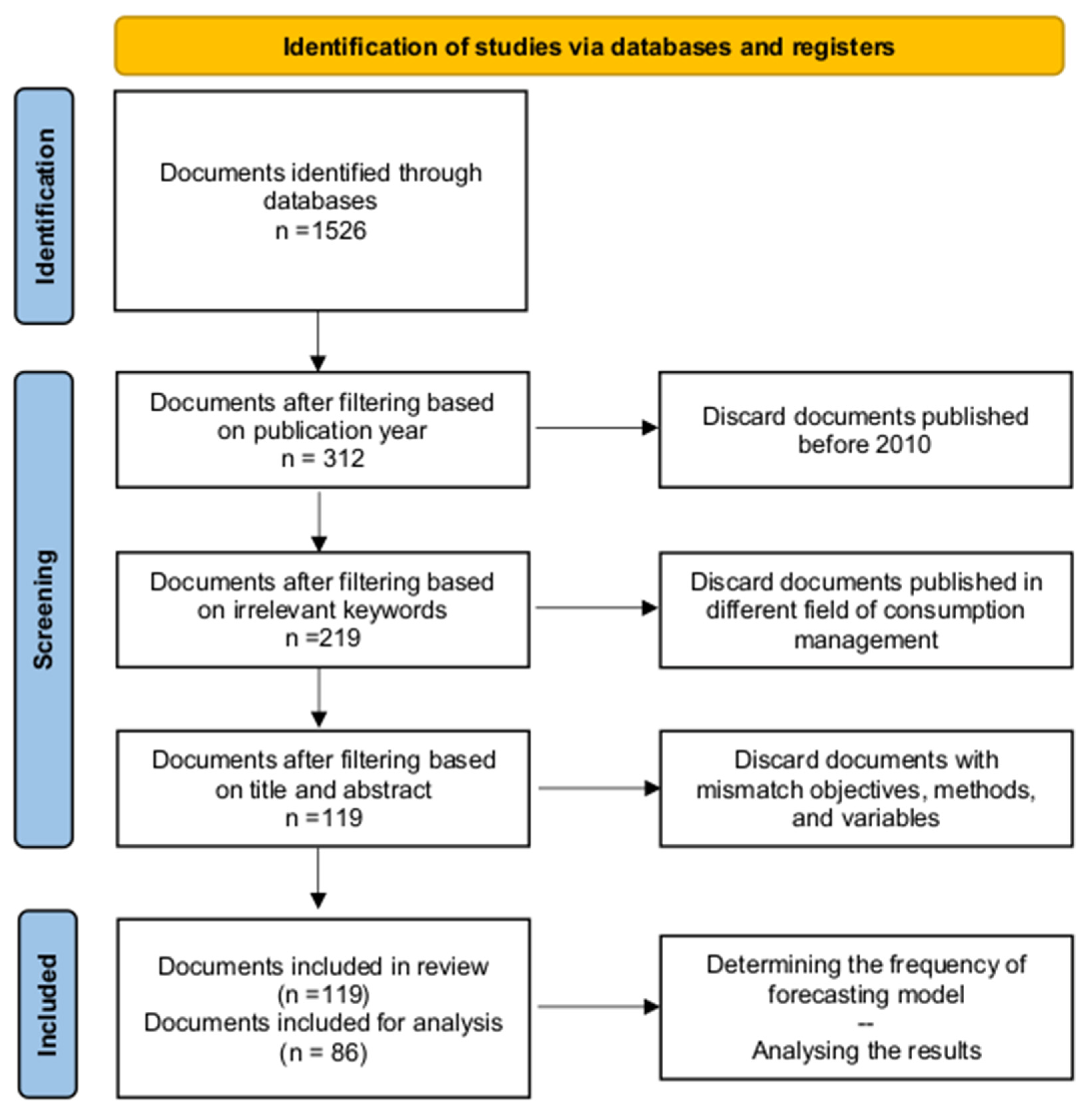
2. Systematic Literature Review: Methodology

This section describes the process of conducting this research, including how articles were collected, filtered, and analysed. Accordingly, the process of conducting this research included three stages: collecting related research from various databases; evaluating and selecting research in accordance with the objectives of this study; and presenting the results of the review and analysis. Figure 2 shows the scheme of the systematic literature review process followed in this paper.

The first stage of the systematic literature review involved the definition of keywords and databases to seek related papers. The keywords were selected in accordance with the objectives of this study. Those comprised of urban water, water supply, water demand, water consumption, demand prediction, predictive methods, predictive models, forecasting, and short-term, among others. The databases used for this search were Web of Science, Scopus, ProQuest, GoogleScholar.com, Google.com, Science Direct, IEEE Xplore, MDPI.com, and ACM Digital Library. The search was performed on these databases by combining multiple keywords with Boolean operators “AND”, “OR”, and “AND NOT” in the title, abstract, and keywords. Only publications post-2010 and in English were eligible within the search.

The second stage shows how the irrelevant articles were deleted. First, to identify the most updated publications, all the articles published before 2010 were discarded. Then, articles were filtered based on irrelevant keywords. For example, articles related to groundwater or articles related to the repair and maintenance of water supply networks were excluded. Finally, the articles were skimmed through their title and abstract to see whether the variables and forecasting methods used in them were in accordance with the objectives of this study.

Table 1. Top 10 journals cited in the current literature review.

Journal Name	References	Publisher	Impact Factor (5 year)	Best Quartile
Procedia Engineering	[12]	Elsevier	-	-
Water Resources Planning and Mgmt.	[11]	ASCE	3.563	Q2
Water	[8]	MDPI	3.229	Q2
Environmental Modelling & Software	[7]	Elsevier	6.036	Q1
Hydrology	[6]	Elsevier	6.033	Q1
Water Resources Management	[4]	Springer	3.868	Q2
Water Supply	[3]	IWA Publishing	1.152	Q4
Water Resources Research	[2]	Wiley	6.006	Q1
Desalination	[2]	Elsevier	9.189	Q1
Sustainable Cities and Society	[2]	Elsevier	7.308	Q1

introduces the top 10 journals in which the articles used in this literature review were published. It is also worth mentioning the wide international representation of case studies that came as a result of this literature review. In this regard, the top 5 countries that appeared more often in the review were the following: Canada (13% of the total of papers in the literature review), Spain (10%), Brazil, China, and UK (each of them at 8%). Tables 2 and 3 provide particular information about the location of the study areas used in part of this literature review.

The third stage discussed the methods and validation indicators that were used in the studied articles. In addition, this stage included a definition and classification of water demand forecasting methods, since the purpose of this paper is providing guidance to researchers and practitioners. Beyond just conducting the systematic literature review, the document provides a critical view of the current and future challenges for water demand. This is of vital importance for water utilities seeking to leverage the emergence of new smart technologies for the operation and management of urban water infrastructure.

3. Predictive Methods and Validation

Most of the literature working on predictive models for water demand forecasting encompassed comparisons between multiple methodologies and an assessment about which performs better for the case studies the authors may have introduced [2,9,12,13]. This section reviews the methods and models used for water demand forecasting during the years 2010–2021, in addition to providing information on validation methods used to check the goodness of fit, or, in other words, to calculate the difference between the observed values and predicted values of any model as well as with their comparison and selection. Previously to enumerate and describe the different predictive methods found in the literature, it is worth mentioning the common factors that all these methods will have, as they need to consider the peculiarities associated with urban water demand. These revolve around the exogenous factors affecting the historical time series data of water demand.

3.1. Impact of Exogenous Factors in Water Demand Models

This section provides an overview of exogenous factors, or covariables, having an impact on predictive models of urban water demand. Such factors range from weather conditions to the geographic locations of the study areas. Economic, socio-demographic, physical, and technological covariables were also shown to be relevant actors in the development of methods for the prediction of urban water demand. According to the classification provided by Bich-Ngoc and Teller [14], the factors having an influence in predicting water demand are classified into six groups. These include climatic or weather, economic, socio-demographic, household properties, technological, and location or geographic factors. A factor that is not included in the aforementioned categories is the calendar variable: weekdays, weekends, holidays, and special events. The descriptions of such factors are the following:

• Climatic or weather conditions (e.g., temperature, humidity, and precipitation): There is almost an evident correlation between weather and water use, and often this is co-founded to customer behaviour and a general seasonality effect on outdoor activity. However, the exposure to severe weather periods will also have a significant impact on the water demand. Climatic variables are among the most used, along with historical past water consumption, and they have been considered in many studies. For example, Brentan et al. [15] examined the correlation between weather factors with water demand and showed that three factors, temperature, relative humidity, and hour of the day, are the most relevant variables for forecasting water demand. Moreover, Hu et al. [16] used temperatures, dew point, humidity, wind speed, and atmospheric pressure as input variables in the water demand forecasting model.
• Economic inputs (e.g., water price, billing, and income): One of the reasons why economic factors, such as price, can be naturally considered for water demand forecasting is due to the fact that a higher price may lead to lower consumption [14]. In some studies, these factors have been considered too. For example, de Maria André and Carvalho [17] showed that some factors, including water price and household income, have a positive effect on water demand, since an increase in these variables will increase water demand.
• Social-demographic situation (e.g., population, household size, and occupants’ ages) and other household properties (e.g., house type and property value): In this regard, Hussien et al. [18] investigated the effect of social-demographic factors, such as the number of children, adult male members, adult female members, and elderly household occupation, as well as some physical property factors, such as household size, household type, the total built-up area of all floors, garden area per household, number of rooms, and number of floors, on per capita water consumption. Additionally, Bennett et al. [19] has introduced the number of adults, children, and teenagers in a household as independent variables for a model based on neural networks.
• Geographical factors (e.g., urban density, and type of location): In the literature, geographical factors have been shown to have an impact on forecasting water demand, and they should be considered further for efficient water supply planning and management [20]. One of the main examples including geographical factors for water demand forecasting is the work of Bao and Chen [21]. They used spatial econometric models to analyse the influencing factors in water consumption efficiency and found that urbanisation level is one of the most important covariables affecting water consumption among the socio-economic and eco-environmental indicators. Among the more relevant works that include GFs in the methodology development for water demand forecasting, Benítez et al. [22] considered the type of location, including the city centre site, the production site (industrial), and the residential site (suburb) to develop predictive models for water demand.
• Technological factors (e.g., smart meters, sensors, and data loggers): Smart meters are the most widely used technological factor among the others. Hence, they have been included in multiple research endeavours on water demand forecasting models. In these studies, users’ consumption information is collected hourly or even instantaneously through such smart meters and used as consumption input data in the forecasting models [13,23]. Other technology factors, such as high-efficiency fixtures and appliances [24] or alarming display monitors [25], have been shown to also have an impact on water consumption. However, such factors have rarely been used in water demand forecasting models.
• Calendar variables (weekdays, weekends, holidays, and special events): Although calendar information is inherently present in other factors, such as weather, socio-demographic, and geographic factors, it is a good practice to specifically consider its effect on water demand models. Calendar variables can be considered as information at a finer granularity than other related factors, having the potential to increase the accuracy of any predictive method. Among the studies that have specifically considered calendar factors, we highlight the works of Pesantez et al. [13]; Benítez et al. [22]; Antunes et al. [12]; Hu et al. [16]; Brentan et al. [15]; Liu et al. [26]; and Herrera et al. [9].

All the aforementioned factors need to be considered as inputs of the predictive methods. The particularities on using these factors will affect the way in which a predictive model is adapted from its general version. An additional challenge is not only using such factors individually but also considering their interactions, for instance how weather variables and population impact water demand in holidays destinations [27]. At a short-term level, water demand will depend on any important social event live or on TV. Last, but not least, water demand is noticeable depending on policies such as the recent worldwide lockdown, with the COVID-19 crisis that kept people at home, and their consequent variation in the water demand profile [28].

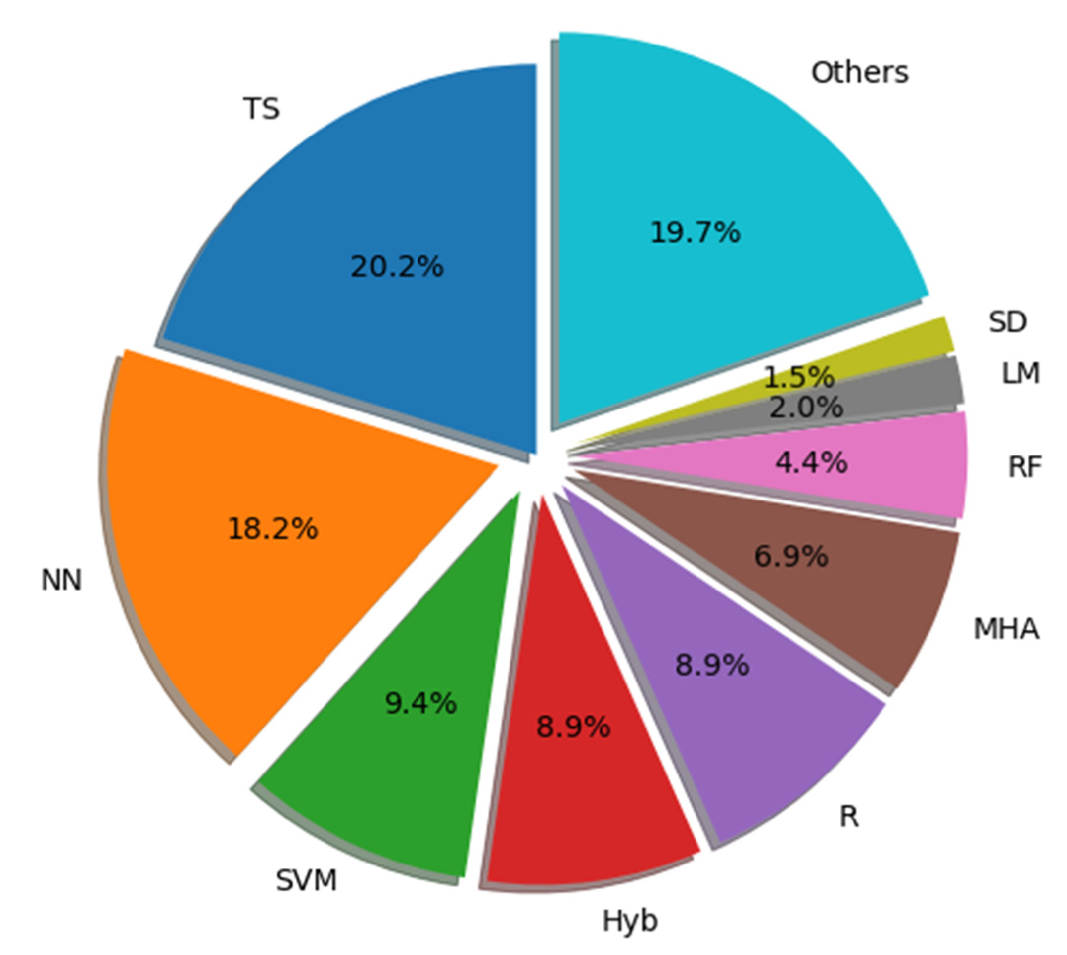
3.2. Predictive Methods for Forecasting Urban Water Demand

There is a plethora of published research in forecasting methods for urban water demand.

Table 2. Summary of factors affecting water consumption and short-term water demand forecasting models. The symbol ‘*’ means that the column feature is included in the revised literature (in rows).

Authors (Year)	Study Area	Measures of Accuracy	Time Periods				Methods
			Hourly and Less	Daily	Weekly	Monthly	TS	NN	R / RF	Hyb	SVM	MHA	LM	SD	Others
Shirkouhi et al. [29]	Canada	RRMSE, MAPE, and NSE	*					*		*		*			*
Koo et al. [30]	Korea	RMSE, NRMSE, NSE, r, and Residual	*				*	*							*
Pandey et al. [31]	Spain and India	RMSE, MAE, and MAPE	*			*	*			*					*
Rezaali et al. [32]	Iran	RMSE, r, NSE, MAE, and MARE	*					*	*		*		*
Du et al. [33]	China	MAPE, MAPE of peaks, r, and explain variance score (EVS)		*				*
Hu et al. [34]	China	MAE, RMSE, NSE, and r	*					*			*
Al-Ghamdi [35]	Saudi Arabian	RMSE		*				*
Salloom et al. [36]	China	MAPE	*					*
Pesantez et al. [13]	United States	RMSE	*				*	*	*		*
Bata et al. [37]	Canada	MAPE and NRMSE	*	*			*		*	*
Xenochristou et al. [38]	UK	MAPE, MSE, and R2		*					*
Yousefi et al. [39]	Canada	CC, RMSE, and MAE	*	*					*			*			*
Pacchin et al. [40]	Italy	MAE and RMSE	*					*							*
Villarin and Rodriguez-Galiano [41]	Spain	R2 and RMSE		*					*
Perea et al. [42]	Spain	SEP and R2		*				*		*		*			*
Maruyama and Yamamoto [43]	Japan	ARE		*		*			*
Gharabaghi et al. [44]	Canada	MAPE, R2, VAF, AICc, and UI & UII		*			*			*					*
Banihabib and Mousavi-Mirkalaei [45]	Iran	RMSE, MARE, MaxRE, MBE, and R2		*			*	*
Benítez et al. [22]	Spain	MAPE, RMSE, and FOB		*			*								*
Candelieri et al. [46]	Italy	MAPE	*				*			*	*
Hu et al. [16]	Not mentioned	MAE and MAPE		*	*			*							*
Kozłowski et al. [11]	Poland	R2		*			*
Antunes et al. [12]	Portugal	RMSE and NSE		*				*	*		*	*
Vijai and Sivakumar [2]	EU	RMSE, R2, MSE, and MAE	*	*				*	*		*		*
Brentan et al. [47]	Brazil	SDe		*			*		*
Sardinha-Lourenço et al. [48]	Portugal	R2 and MAPE	*				*								*
Shabani et al. [49]	Canada	MAE, RMSE, R2, and MAPE	*				*			*		*
Pacchin et al. [50]	Italy	RMSE and MAE	*												*
Oliveira et al. [51]	Brazil	MAPE and RMSE		*			*			*		*
Gagliardi et al. [52]	UK	NSE	*					*							*
Brentan et al. [15]	Brazil	RMSE, MAE, and R2	*				*			*	*
Candelieri [23]	Italy	MAPE	*				*				*
Tiwari et al. [3]	Canada	R2, RMSE, Pdv, MAE, and PI		*				*					*
Arandia et al. [53]	Ireland	RMSE, NRMSE, and MAPE		*	*		*
Walker et al. [54]	Greece	CC and Sde	*					*		*		*
Candelieri et al. [55]	Italy	MAPE	*				*				*
Hutton and Kapelan [56]	UK	MAPE	*				*
Al-Zahrani and Abo-Monasar [57]	Saudi Arabia	MAPE and R2		*			*	*
Vijayalaksmi and Babu [58]	India	RMSE, MAPE, and CC		*				*
Tiwari and Adamowski [59]	Canada	R2, RMSE, Pdv, MAE, and PI			*	*		*		*					*
Bakker et al. [60]	Netherlands	RE, MAPE, and R2		*			*		*						*
Romano and Kapelan [61]	UK	MAPE and MSE	*				*	*
Okeya et al. [62]	UK	MAE	*				*								*
Bai et al. [63]	China	NRMSE, CC, and MAPE		*			*		*			*
Candelieri and Archetti [64]	Italy	MAPE	*				*				*
Chen and Boccelli [65]	Not mentioned	AARE	*				*
Alvisi and Franchini [66]	Italy	NSE and RMSE	*					*		*					*
Sampathirao et al. [67]	Spain	Average PMSE24, Average PRMSE24, and Number of Parameters	*				*	*		*	*				*
Bennett et al. [19]	Australia	R2, ARE, AAE, RMSE, Mann–Whitney, Wilcoxon (MW), and p-value		*			*
Liu et al. [26]	China	AARE	*								*
Khan et al. [68]	Australia	Ac		*				*	*		*
Adamowski et al. [69]	Canada	R2, RMSE, RRMSE, and E		*			*	*	*						*
Azadeh et al. [70]	Iran	MAPE		*				*	*						*
Odan and Reis [71]	Brazil	MAE and r	*				*	*
Herrera et al. [72]	Spain	RMSE and MAE	*				*	*		*
Herrera et al. [9]	Spain	RMSE and MAE	*				*	*	*		*
Adamowski and Karapataki [73]	Cyprus	R2, RMSE, AARE, and MaxARE			*			*	*
Caiado [74]	Spain	MSE		*			*
Wu and Yan [75]	United Kingdom	MSE, RMSE, MRE, and MaxRE		*								*

and

Table 3. Summary of factors affecting water consumption and medium-term and long-term water demand forecasting models. The ‘*’ symbol means that the column feature is included in the revised literature (in rows).

Authors (Year)	Study Area	Measures of Accuracy	Time Periods			Methods
			Monthly	Quarterly	Yearly	TS	ANN	R/RF	Hyb	SVM	MHA	LM	SD	Others
Shuang and Zhao [76]	China	MSE–MAE-R2			*			*		*				*
Ristow et al. [77]	Brazil	MAPE	*			*
Karamaziotis et al. [78]	Greece	MAE, MASE, RMSE, and MAPE	*			*
Sanchez et al. [79]	United States	ST			*			*						*
Guo et al. [80]	China	B, RE, and MRE			*						*
Rasifaghihi et al. [81]	Canada	Silhouette coefficient			*	*		*						*
Duerr et al. [82]	United States	RMSE, GINI, AWPI, ECPI, and NOIS	*			*		*				*
Sharvelle et al. [83]	United States	MRE, bias fraction (BIAS), and NSE	*											*
Haque et al. [84]	Brazil	R2, RMSE, MARE, and NSE	*					*
Shabani et al. [85]	Canada	R2 and RMSE	*							*
Yousefi et al. [86]	Canada	R2, RMSE, and MAE	*								*
Nassery et al. [87]	Iran	ME, MAE, MAPE, and RMSE	*	*									*
Altunkaynak and Nigussie [88]	Turkey	RMSE and NSE	*			*	*		*
Vani [89]	India	-			*								*
Fullerton Jr et al. [90]	United States	B and ST	*			*
Peña-Guzmán et al. [91]	Colombia	RMSE, AARE, and R2	*				*			*
Shabani et al. [92]	Canada	R2, MAE, RMSE, and NSE	*							*	*
Shabri et al. [93]	Malaysia	RMSE, MAE, and CC	*				*			*
Kofinas et al. [94]	Greece	R2, MAPE, RMSE, and MAE	*			*	*		*
de Maria André and Carvalho [17]	Brazil	LM, Moran-I test, and R2	*	*		*								*
Yang et al. [95]	Not mentioned	-			*								*
Almutaz et al. [96]	Saudi Arabia	SDe	*											*
Nasseri et al. [97]	Iran	B, NMSE, and R2	*			*			*		*			*
Qi and Chang [98]	United States	Compared with Real-world water demand data			*								*
Firat et al. [99]	Turkey	AARE, NRMSE, and Ts	*			*	*
Varahrami [100]	Iran	RMSE, MAE, and MAPE	*				*		*		*
Mohamed and Al-Mualla [101]	Emirates	AARE, ARE, and SDARE	*		*									*

summarise the validation indicators and predictive methods used for short- and long-term demand prediction. These methods and indicators are further classified, reviewed, and discussed.

Figure 3 shows a classification of the main works based on the frequency of their use in the reviewed articles in Table 2 and Table 3 and the type of method used in these articles. The most widely used methods, presented below, include diverse types of artificial neural networks (ANN), traditional time series (TS), regression (R), support vector machines (SVM), hybrid models (Hyb), metaheuristic algorithms (MHA), machine learning (ML), and system dynamics (SD).

The classification above is based on basic models that are also extended to particular approaches. For instance, methods based on neural networks encompass long short-term memory [33], radial basis function ANN [30], and gated recurrent units [36], all of them included in the ANN class. Methods based on time series encompassing probabilistically exploratory TS [56] and exponential smoothing state-space models [77] were included in the TS class. The classification of other methods, such as SVM, Hyb., and others, was similarly performed. Of course, other methods fall out of the main classifications and are consequently included in the class “others”. Among these methods, it is worth highlighting the homogeneous and non-homogeneous Markov chains [52] and the nonlinear local approximation method [39].

3.2.1. Artificial Neural Networks

Artificial neural networks (ANNs) are machine learning models for clustering, classification, and prediction. The simplicity in their overall design, and a high performance level, made them into one of the most widely used predictive methods in water demand. ANNs are inspired by how the human brain and nervous system work. An ANN is, then, an interconnected assembly of artificial neurons, arranged in a series of layers in which the elements from one layer are fully connected to the elements of the other. The data is presented to the ANN at the so-called input layer, transmitted to a hidden layer, where it is transformed, and again forwarded to compute an outcome (prediction in this case) at the output layer. At the output layer, an estimation error is computed, and the ANN method uses a back-propagation process to learn how to optimally adjust the interconnections weights [9]. This is an iterative feed-forward training plus back-propagation validation process until convergence. In the literature, it is possible to find a myriad of combinations and choices for the creation of different families of ANNs and combinations with other machine learning and statistical processes.

One of the benefits of using ANNs is their accurate predictions with little or no prior knowledge of the problem. However, ANNs’ performance is significantly superior after their adaptation to a specific problem to solve and to the data available, rather than directly using the standard procedure. Such an adaptation may require bringing knowledge to the input layer in terms of historical data at relevant time-series lags and information of covariables such as climate and calendar information. On the downside, ANNs face issues related to their lack of explainability, the large quantity of data often needed for their training and validation, and the risk of having a lack in generalisation of the findings out of the range of the observed data [10].

Salloom et al. [36] used a new machine learning method named Gated Recurrent Unit (GRU) as a basic model for forecasting hourly water demand in Changzhou, China. The gated recurrent unit (GRU) is an effective chained deep learning model that considers the previous information and is suitable for sequence data analysis. It has a reset gate and updates gate phases to avoid vanishing and exploding gradient problems, and it can determine what information should be passed to the output. The results of their study showed that this new method reduces the complexity of the prediction model six times than that achieved in the literature while conserving the same accuracy. Hu et al. [34] also applied the GRU for forecasting the hourly water demand of District Metering Areas (DMA) in Shanghai, China. They compared the result of the GRU with SVM and traditional ANN and showed that the GRU-based models are more accurate than the two other models.

3.2.2. Support Vector Machines

Support vector machine (SVM) methods were introduced as a classification method in the mid 90 s, firstly as an innovative approach for solving a single perceptron problem associated with an ANN. SVM gained generalisation power by working with kernel functions, enabling it to perform at least at the same accuracy level as an ANN for classification [85] and regression and support vector regression (SVR). The way in which such kernels (similarity function of the input space data) work for SVMs is by a mapping of the problem domain with complex, non-linear relationships into a high dimensional space in which the computations needed to solve such a problem are easier and, ultimately, of a linear nature [102].

Several studies have shown the excellent performance of SVR in water demand forecasting. This is the case of Liu et al. [26] who used a set of SVR models to forecast daily demand patterns and to infer the factors of higher influence. Herrera et al. [103] worked with a multiple kernel regression for which single kernels were computed per each different type of input data and combined into a single, multi-kernel regression model [104]. Similarly, Shabani et al. [85] predicted the monthly water demand via SVM using a polynomial kernel function. In their study, several combinations of SVM models were tested to assess the impact of lag time in the inputs data and compare the performance of these models. Based on the results, it was found that different combinations of input variables affect the performance of the SVM model for forecasting. Candelieri and Archetti [64] and Candelieri et al. [55] introduced a two-stage framework for hourly water demand forecasting. First, the demand pattern was characterised through a time series clustering. Second, they ran an SVR model to predict the water demand at each cluster previously found. They showed that by using this two-stage framework, it is possible to make a reliable forecast of water demand and the consequent optimisation of water supply operation and management. In a further work, Candelieri et al. [46] developed a parallel global optimisation process for tuning the SVR hyperparameters to significantly reduce the forecasting errors of the final predictive model.

There are multiple works about SVMs in combination with other machine learning methods. Despite that the current paper has a dedicated subsection to hybrid methodologies, we emphasise here the relevance of such combinations in the application of SVM and SVR in urban water forecasting models. Shabri et al. [93] applied a combination of an empirical mode decomposition (EMD) and a least square support vector machine (LSSVM) model to the problem of monthly water demand forecasting. The proposed EMD-LSSVM model outperformed the EMD-ANN as well as the LSSVM and ANN models. Another example is the work of Peña-Guzmán et al. [91], in which the author used LSSVM to predict residential, industrial, and commercial monthly water demand. They proved that the LSSVM model was superior to an ANN model in terms of accuracy. Brentan et al. [15] applied an SVR model for hourly water demand forecasting. They added a Fourier time series process over the SVR model to improve the base prediction and to make it responsive to near-real-time predictions. They showed that this procedure reduces the near-real-time prediction errors as well as any biases developed over time, common for fixed regression structures.

3.2.3. Traditional Time Series Analysis

Time series (TS) models are broadly defined as those methods based on the analysis of historical data. Most of the demand forecasting methods fall into this category. In the following, we use the term TS analysis to refer to the more traditional procedures to work in this topic. Those imply an analysis by the decomposition of their main statistical elements, namely level, trend, seasonality, and noise. Traditional TS analyses do not reach the high accuracy levels that many of the machine learning-based models may bring, due to traditional TS struggle to capture nonlinear relationships for demand forecasting. However, a clear advantage of traditional TS relies on their great explainability. This cannot be overviewed, since one of the aims of the forecasting process is often related to obtaining a proper model explanation, fostering model confidence, and an overall better-informed decision-making process.

The autoregressive integrated moving average (ARIMA) models are methods widely used in traditional TS analysis and forecasting. Several developments come associated with ARIMA models by adding certain parameters. To mention a few, SARIMA considers a stational component of the time series, and ARIMAX adds exogenous covariables. In the case of water demand forecasting, ARIMAX models are of main importance since they can include covariables such as weather factors and social demographic factors that showed to be key for the predictive performance of the models [105].

In the literature on urban water demand, there are multiple works that use traditional TS as the main forecasting method. Chen and Boccelli [65] developed an integrated TS forecasting framework for hourly/quarter-hourly demands of a medium-size water supply system. The models used in their research were a fixed and an adaptive seasonal autoregressive model, and both were suitable for use in water utilities running SCADA. Okeya et al. [62] used a TS model to forecast water demands at 15-minute intervals in a water distribution system. They used two data assimilation (DA) methods including a Kalman filter, a linear quadratic estimation in principle designed to control sources of uncertainty in TS forecasting, and an ensemble Kalman filter. Their aim was to improve the real-time of water demand prediction and the estimation of hydraulic system states. Arandia et al. [53] used a Kalman filter, as a DA, combined with a SARIMA model to predict water demand both for online and offline modes. They predicted quarterly, hourly, and daily demands analysing the output in a variety of time resolutions.

The use of ARIMA for water demand was key in the works of Banihabib and Mousavi-Mirkalaei [45], who proposed ARIMA and nonlinear auto regressive exogenous models for daily urban water consumption forecasting. Karamaziotis et al. [78] examined several methodologies, including ARIMA, exponential smoothing, and multilayer perceptrons. Fullerton Jr et al. [90] used a developed time series model named linear transfer function ARIMA to simulate the monthly frequency of water demand. They showed that the model performs well in predicting customers’ demand but falls in predicting consumption growth, since the model may need regular updates to address such a bias.

Ristow et al. [77] developed two models based on time series for predicting monthly water demand of the four consumption categories, including residential, commercial, industrial, and public, as well as total consumption, in the city of Joinville, Brazil. One of the employed models was the exponential smoothing state-space models (ETS), and the other was performed through the Box–Jenkins methodology (ARIMA models). The result of their study showed that the seasonal ARIMA method (namely SARIMA) is performed more adequately to predict water consumption in these categories, except that in the residential category, and it can be applied to monthly urban water consumption forecasts.

3.2.4. Metaheuristic Algorithms

Metaheuristic or evolutionary algorithms (e.g., genetic and swarm-based algorithms) are a group of decentralised intelligence methods whose operations are inspired by natural phenomena, usually through mimicking a collective behaviour of a system or organism. Such a system behaviour brings intelligence and adaptation for the total of any system, which cannot be reached by the mere addition of its single parts. Metaheuristic algorithms search the solution space and often find near-optimal solutions to non-deterministic polynomial time problems [106], normally used for the design and optimisation of water distribution systems. The main advantages of using metaheuristic algorithms are the ability (i) to search the entire solution space and thus find excellent quality solutions with a high probability; (ii) to link to and combine with other methods; and (iii) to reach high flexibility to solve multi-objective problems related water systems operation and management [107].

In water demand forecasting, Romano and Kapelan [61] directly used metaheuristic algorithms to estimate water demand for the next 24 h period. They particularly used evolutionary artificial neural networks. However, metaheuristic algorithms are often found in combination with other machine learning methods, such as ANN or SVM, to adjust their hyperparameters [102]. Varahrami [100] presented two types of neural networks tuned with a GA to predict the monthly water demand. Wu and Yan [75] applied two genetic programming (GP) approaches, including tree-based genetic programming (TGP) and gene expression programming (GEP) for daily demand forecasting in a district metered area of a water distribution system. Nasseri et al. [97] predicted the monthly water demand using a method consisting of GP and an extended Kalman filter (EKF). They used EKF to infer latent variables in a forecasting model that was formulated using GP. Shabani et al. [49] proposed an approach based on a two-stage learning process that couples GEP with time-series clustering for short-term water demand forecasting. In the proposed a two-stage approach, time-series clustering is used to organize daily water demand patterns with gene expression programming to model the demand of such clusters. The results proved that GEP can provide a high accuracy while coupled with unsupervised learning algorithms.

Bai et al. [63] proposed a model based on wavelet transformations to train a relevance-vector regression for predicting urban water demand at different scales, multiscale relevance-vector regression (MSRVR). Then, they used an adaptation of a particle swarm optimization (PSO) algorithm to optimise the parameters combination of such a model. The proposed MSRVR-PSO had better performance in predicting water demand than variations of ANN models specifically tailored for regression analysis.

3.2.5. Regression

Regression models estimate how changes in a group of independent variables may have an impact on the dependent variable, which is usually of interest. These models are suitable for predicting future demand, although such predictions should remain under a certain time stretch to keep their validity. This is due to the fact that the predictions are mainly extrapolations out of the regression input domain where the structural stability of the independent variables is of the main importance. That is to say, the assumption for which the relationship between the variables involved in the regression and their impact into the dependent variable is still the same as in the range of observed data. The use of regression methods is, hence, common for short-term demand forecasting.

Bakker et al. [60] studied a multiple linear regression (MLR) model along with an adaptive heuristic algorithm searching to optimise a transfer function-noise (TFN) model (taking the independent variables at different time lags). The authors used these methods for the water demand forecasting of a benchmark of district metered areas for water utilities. The results showed a higher accuracy for the combined heuristic-TFN model than MLR at forecasting the one-day lead water demand. The interest of this outcome lies on the possibility to increase the predictive power without a loss of model explainability. Maruyama and Yamamoto [43] also used MLR-based models for better management of the daily water supply. Rasifaghihi et al. [81] used a Bayesian regression to forecast the daily urban water consumption. In a Bayesian framework, the regression model is similar in structure to the frequentist, least-squares regression analysis. However, the Bayesian model parameters have a certain probability distribution, and they are updated in the actual regression process by the likelihood of the observations.

Haque et al. [84] applied the independent component regression (ICR). This is a method that brings to the analysis the capacity of separation of the input domain into additive parts able to reconstruct the variable of interest (dependent variable) in a way in which it can be used for regression analysis. The authors used ICR as a main method for urban water demand forecasting. They compared the performance of ICR to two other regression methods: principal component regression (PCR, that is, MLR with the principal components covariables as input) and MLR. The results showed ICR having the best performance in comparison to PCR and MLR.

Among the multiple options for regression analysis in forecasting, SVR and random forest (RF) are the two methods of great success in the water demand literature. Having above a subsection specifically dedicated to SVR, it is necessary to introduce RF now. RF is an ensemble of decision tree (DT) models which split, in a recursive manner, the input space into a tree-like hierarchy of subsets. This partitioning process creates the so-called leaves of the tree in which it takes place a subset classification or regression. An RF makes an ensemble of many DTs, each one computed after a random selection of independent variables. It has been proven that in many classification and regression tasks, RFs are outstanding predictive models [9].

Like many other forecasting methods, this technique has also been used to predict water demand, and its performance has often been compared to other forecasting methods. Brentan et al. [47] proposed an approach to distribution network modelling and water demand forecasting, using RFs to investigate the relationship between climatic variables. As a result, they showed that this artificial dataset can be used as input data for addressing hydraulic analysis further. Interestingly, Antunes et al. [12] and Pesantez et al. [13] developed an RF-based technique combined with other methods. They showed that a mixed technique presents a high level of efficiency and accuracy. However, Vijai and Sivakumar [2] showed that ANNs had a better performance than other methods, including simple RF and other RF-based methods.

3.2.6. Hybrid Methods

A hybrid method integrates various models (e.g., artificial neural networks and traditional time-series models; several regression methods; and metaheuristic algorithms and artificial neural networks) to use the advantage of each of these techniques as they are used simultaneously. Actually, theoretical and empirical results from various research works have shown that a combination of methods can effectively improve the accuracy of a predictive model [48] and, in general, outperform the methods used separately. For example, Herrera et al. [72] proposed a hybrid method based on a traditional ARIMA time-series approach and ANNs to predict the municipal water demand. They used ARIMA to analyse the linear part of the problem as the basis of water demand time series, while the ANN modelled their residuals. The proposed hybrid model could predict demand more accurately than the ANN and the ARIMA models used separately. An added advantage of the use of this combination of ARIMA + ANN is that ARIMA will supply a suitable explanation for the linear part of the resulting model. Equivalent results were also found by Kofinas et al. [94], who estimated monthly urban water demand.

Oliveira et al. [51] applied a double SARIMA model to predict water demand and used the Harmony Search (HS) algorithm to estimate the parameters of the SARIMA model, where HS had an effective role in improving the performance of the predictive model. Sardinha-Lourenço et al. [48] showed that a parallel combination of the heuristic model with an ARIMA model, and an efficient weighting calculation method, improved the performance of the predictive model. With respect to hybrid methods in which ANN is involved, Odan and Reis [71] presented two models, ANN-H and DAN2-H, made by combination of a Fourier series with an ANN and with a dynamic ANN, respectively. They found that the dynamic ANN combination had the best performance for hourly demand forecasting. Azadeh et al. [70] proposed a hybrid model to predict daily water consumption for warm and cold days. They combined an ANN, a fuzzy linear regression (FLR), and an analysis of variance (ANOVA) to construct a hybrid model. They showed that the hybrid approach was suitable to predict demand under nonlinearity and uncertainty conditions. Another example is the work of Perea et al. [42], who successfully introduced a Bayesian framework for a hybrid model made by a combination of a dynamic ANN and a GA.

Other actors for the hybrid method were those proposed by Bata et al. [37], who worked in a model that consists of a regression tree (RT) over self-organizing maps (SOM). In this model, the SOM method was used to group the water outflow input data into clusters, and the RT method predicted the water demand considering such groups. The output of the SOM clustering method was the input for RT. The outputs coming from the use of SOM significantly improved the performance of the standalone RT and SARIMA models.

Additionally, Shirkouhi et al. [29] proposed a hybrid method for short-term urban water demand prediction in two cities of the Quebec province (Canada). They used the Genetic algorithm (GA) for the optimization of the ANN model’s hyperparameters and compared the performance of this model with the ARIMA model and a pattern-based model named the fully adaptive forecasting (FAF) model. Based on the results, it was determined that the optimization of the hyperparameters of this ANN model with the Genetic algorithm can improve the accuracy of the prediction.

Pandey et al. [31] improved two hybrid models for forecasting hourly and monthly water demands. The first model was combined the ensemble empirical mode decomposition (EEMD) and difference pattern sequence forecasting (DPSF) methods, and the second was based on the combination of EEMD and DPSF, as well as ARIMA. They used two data sets, including the hourly water consumption of a city in southeastern Spain and monthly water consumption of Nagpur, India, for evaluating the performance of these two models. They compared the results of these two methods with the predictions obtained from a number of available models, including PSF, ARIMA, DPSF, and ANN models. The results showed that the EEMD-DPSF method is performed better than the other methods in terms of prediction accuracy.

3.3. Model Validation

Validation indicators calculate the forecast error rate that is the difference between the forecast value and the actual value. Such indicators play, then, a key role in the validation and selection of the forecasting method. Table 2 and Table 3 summarise and classify the validation indices more often used in the literature (Figure 4).

Figure 4 shows that the highest percentage of use of validation indicators are related to the root mean squared error (RMSE), coefficient of determination (R²), mean absolute percentage error (MAPE), mean absolute error (MAE), and Nash–Sutcliffe efficiency (NSE) indices. The lower the RMSE, the better the fit of the model to the observed data. Note that RMSE is scale dependent and it is suitable, in principle, just to compare models using the same dataset. The R² is a non-dimensional number between 0 and 1, being the proportion of the observed variability explained by the predictive model. Hence, the closer R² is to 1, the better the model performance. MAPE considers the error in terms of proportions or percentages, also being a non-dimensional measure. The lower the MAPE value, the better the forecast. The MAE criterion is similar to RMSE but considering the absolute value. Hence, MAE will be more tolerant than RMSE to individual errors in the summation since their values are not squared. NSE represents the gain of using the model vs. using the mean. NSE = 1 is associated with a perfect fit. NSE = 0 indicates that the model has a similar performance as the mean of the historical time series. Abbreviations includes a full list of the validation indicators in the literature.

3.4. Peaks of Water Demand

On a regular basis, both predictive and validation methods address the development of models by focusing on predictions for the mean or median. Being useful in most of the cases, this approach falls short when the management or operation issue is near or on the peaks of the water demand profile [59]. This is due to the fact that the mean-/median-based methods naturally tend to make predictions smoother at the peaks. At the same time, validation indicators usually refer to the mean/median, rather than to another, more-extreme quantile, as the loss function to minimise in a method that calls for such a validation. Nevertheless, the quantile regression approach is an underexplored methodology in the literature of water demand. Quantile regression is a generalisation of the least-squares regression conditioned on every quantile of the dependent variable, rather than conditional to the mean as happens in the classical regression models [108].

Depending on the time scale, peaks are related to factors such as climate/weather (rainfall, summer, or warm periods). Adamowski and Karapati [73] compared MLR and ANN for estimating the peak of hourly urban water demand and its correlation to extreme weather events such as rainfall occurrence. Other works, as the article by Vonk et al. [27], focused on climate variables and on socio-demographic information (garden area and number of residents), including calendar variables that may explain, for instance, periods of the year in which the city may receive/export tourism.

Peak demand forecasts have been shown in the literature to be key for the cost-effective management of water distribution systems, for instance by the optimisation of water pumping schedules [109]. With a focus on the time-series frequencies, another article about peak water demand is the work of Kozłowski et al. [11]. They proposed TS models based on trend and harmonic analysis to predict water consumption in a supply water system. Using these models, they predicted daily water demand, as well as compared water consumption on different days of the week and consumption at different hours of the day, to determine peak days and peak hours of consumption. They evaluated these models with the statistical tests and concluded that they can effectively be used in water demand forecasting and to design controllers for water supply pumps.

4. Future Directions for Short-Term Water Demand Forecasting

There are multiple challenges coming for the sustainable management of water demand. Some of them are associated with the technologies available today, and some others are coming due to the surge of climate change and the more-frequent-than-ever extreme weather conditions happening worldwide. In all the cases, there is an urgent need for the development of efficient and accurate methodologies aiding utility managers and policy makers in their decision-making process. If the output of water demand forecasting models is accurate, practical applications of these results in the decision-making process can be used. For instance, the expected outcomes of these models will inform an optimal water supply pumping schedule that comes associated with a certain level of necessary precision for the models that is different to the requirements of models addressing predictive models for household water consumption. Examples of other related problems for which a water demand prediction output is necessary as an input are water tank filling, leakage detection, smart metering, and billing. The problem also varies in its statistical objectives, since they vary from average to peak water demand, and from future prediction to data loss interpolation. This section discusses these aspects further.

4.1. Upcoming Challenges for Water Demand Forecasting

Methodologies related to water demand forecasting need to be adapted to new social, economic, environmental, and technological challenges. Hence, the social, economic, and hydraulic goals for which traditionally water demand forecasting has been developed need to be extended to be a main part in a digital and automated framework for the operations and management of water utilities today. There are a few main upcoming characteristics for the latest trends in the water demand management. One is the presence of highly interconnected cyber–physical systems (CPSs), made of smart meters, sensors, and actuators for the monitoring and control of the physical assets in the urban water infrastructure at near real-time. The paradigm shifts in the time-period factor presented in Section 3, since now there is an even shorter period than the hourly basis demand prediction. This change is fundamental to understanding new challenges for water demand forecasting methods that now also become an essential part for tasks such as anomaly detection to complement any intelligent control and predictive maintenance policies that water utilities may already have in place. Furthermore, CPSs come also associated with a network of data sources, coming from such sensors and smart meters, that requires not only a shift in the time-period but also the development of methods able to count on the complete information available in a multivariate stream of time-series signals and data.

Near-real-time models for water demand: CPSs endow water supply with features of a proper smart system, that is, using near-real-time data for the operation of variable speed pumps and dynamic control of valves, as well as reservoirs and water tanks. This will make it possible to have optimal water demand balance, minimise overpressure, and, consequently, achieve water and energy savings. The benefits of a CPS expand to an online knowledge of the hydraulic state and asset condition, both being essential for optimal water supply performance.

Data stream forecasting for water demand: Data streams procedures to deal with water demand are a quite unexplored topic in the literature. However, there is an important research avenue, for instance, by exploring the benefits of multiple models for water demand considering simultaneously time-series data per each of the district metered area (DMA) in which a water distribution system may be partitioned. In addition to modelling the interrelationship between such time series, other research could also be targeted in future. This is the case of the development of transfer learning models considering that patterns demands can be learned by one DMA from another of similar characteristics.

Anomaly detection is a challenge suitable to be addressed by both near-real-time and data-stream models. Related to water demand forecasting, anomaly detection procedures may discover patterns in the time-series data that lead to better operation and management for paradigms ranging from leakage detection to the replacement of malfunctioning valves and to even deal with new threats that represent cyberattacks.

Water demand management is in constant adaptation to meet both the most traditional challenges from a hydraulic point of view for an efficient water supply and the surge of big databases of decentralised time-series data available in streaming. Given this scenario of current and future outstanding challenges for water demand, there comes the question of the relative lack of success so far on the use of deep learning methods for predictive methods of water demand. There are several reasons to answer this point. First, the accuracy shown so far by deep neural networks did not overcome sufficiently the results coming from shallow methods such as ANNs, RFs, or SVR, to mention a few. A second reason is about the huge quantity of data usually required for the proper use of deep neural networks that has not been used in practice so far. Furthermore, deep neural networks were initially designed to approach complex tasks that often do not match with the simplicity of working with water demand management in the traditional manner mentioned above. The surge of working with a digital twin of the real infrastructure and the CPSs management, along with their associated big and interconnected data analyses, should give a boost to deep neural networks in the future. On top of this, the transition to 5G will make the data transmission speed sufficient to use more ambitious methods such as those based in deep learning algorithms.

4.2. So, What Method Should I Use?

There is not a universal response to the question of what method to use. However, the method to use can be selected among those showing better performance with respect to the data available for each case and the (operation and management) objectives to deal with. Only answering the questions of the temporal scope needed and the exogenous factors considered in the database will help to narrow down the general forecasting method to use and, consequently, how this may be adapted to the specific working scenario. Additional questions will continue helping the selection of a suitable forecasting methodology, that is, to answer the question of targeting the development of a model suitable for average or for peak water demand. Other questions to take into account are whether the objective is to create predictive models for water demand forecasting, or whether it is to have an anomaly detection model able to aid any predictive maintenance process for the water supply infrastructure. Other aspects to take into account are those related to the technology available since it is possible to have near-real-time data and/or data coming from multiple water meters. Technology conditions are an opportunity to address more ambitious objectives of the forecasting methods, which should be efficient (in the case of near-real-time work) and should allow parallel computation and learning from other models in a collaborative manner (in the case of data streams). The following bullet points summarise the steps discussed in this paragraph:

• Identification of the temporal scope and (exogenous) factors of influence at each particular use case.
• Objective of the analysis: average vs. peak demand and anomaly detection vs. future prediction.
• Technology available: Requirement of near-real-time models. Solutions for multidimensional data streams.

Table 4. Advantages and disadvantages of the main categories for predictive methods in water demand forecasting.

Method	Data Requirements	Accuracy	Interpretability	Efficiency	Adaptability
ANN-like	High	High	Low	Low	Medium
SVR-like	High	High	Medium	Low	Medium
ARIMA(X)	Low	Low	High	High	Low
Metaheuristics	High	Medium	Low	Low	Low
Regression	Low	Medium	High	High	Low
Hybrid	High	High	Medium	Medium	High

shows a summary comparison of the main methods used for water demand forecasting in terms of the data requirements for the methods to run, accuracy, interpretability of the model, computational efficiency of the algorithm implementation, and adaptability to sudden changes in the water demand. Note that it is the view of the authors after being processed the results of the current literature review. Furthermore, some of the methods are classified in broad categories and it may be that some of the methods of these categories are not being well represented by the summary features of Table 4. This is the case, for instance, of an RF, classified as a regression method, and often providing “high”-accuracy predictive models.

4.3. Recommended Software: R, Python, Julia

After the open discussion on “what model should I use?”, the other main question remaining for researchers and practitioners is about software. The authors of the current literature review paper firmly believe that the decision about the model to use is also related directly to the software of choice. There is a plethora of choices of software on the market. However, in the following bullet points, we only mention the main open-source options, namely those based on R, Python, and Julia.

• The R environment for statistical computing is a free software platform used for statistics and data mining [110]. R is widely used for time-series analysis and forecasting; such is the case of the development of predictive models for water demand. The R community is active in providing programming support and in the number and up-to-date quality of the so-called R packages, which are software libraries developed to run specific methods and data analysis. Among them, they highlight the package “neuralnet” to work with ANN [111], “e1071” to work with SVR [112], or “randomForest” to work with RF [113]. An additional advantage of R working with water demand comes thanks to matching data analyses to the Epanet-toolkit R packages “epanetReader” [114] and “epanet2toolkit” [115].
• Python is an interpreted, general-purpose programming language that can provide a multiplatform solution for scientific computing [116]. This is thanks to Python libraries such as “pandas” and “numpy” for data manipulation and basic analysis and “scikit-learn” [117] for machine and statistical learning software development (including functions to work with ANN, SVR, RF, and many more). Python also has the backup of a huge community supporting up-to-date libraries, creating an ideal framework for research and software development. Importantly, there is a Python library to run the Epanet toolkit called “Epanettools” and a library called “WNTR” that is an Epanet-compatible Python library for the simulation and analysis of water distribution systems resilience, developed by the Sandia National Laboratories and the US Environmental Protection Agency (EPA) [118].
• Julia is a high-level programming language that naturally supports concurrent, parallel, and distributed computing [119]. This means that, although Julia is a general-purpose language, it was originally designed for machine learning and statistical programming. Julia is a quite new language, and it is still far from the popularity of R or Python. However, there is foreseen a brilliant future for Julia given its properties of speed, using just-in-time compilers making it as fast as low-level compiled languages such as C. In addition, Julia can be executed in R, Latex, Python, and C, while Julia can also wrap R and Python code, thanks to the libraries “RCall” and “PyCall”, respectively.

There is not a best choice among these software options. This should depend mostly on what software the researcher or practitioner may feel more comfortable and secure working with and using to develop water demand forecasting tools eventually, along with their wrap for applications in water supply operation and management.

5. Conclusions

Regarding water demand forecasting methods used in the literature, it is not clear which one performs better than others. However, there are several straightforward points that may aid in a method selection process since a common point for any method is the need to adapt both to the available data and to the problem to be solved. A first question is about the temporal scope that the predictive model should target. Then, it is necessary to check the data available, including the exogenous information and covariables to add to the purely historical time-series demand. The method selected also varies with whether the focus is on the peak or average water demand estimations. Different predictive model objectives may also lead to a different method needed for their accomplishment. Hence, anomaly detection comes associated with different main procedures than forecasting for better operation performance. Last but not least, the technology available also plays a fundamental role in water demand forecasting, primarily in a working objective selection and, consequently, in the predictive method to be used.

An interesting finding that emerges from the literature review is the success in using interpretable methods as predictive models of water demand. For the years in which the literature review was addressed, approximately 30% of the papers based their analysis on traditional time-series (e.g., ARIMA models) and regression models (including multivariate regression, decision trees, and random forests). The reason for their success is having a sufficient predictive ability for a range of the operations in water supply management, such as pumping schedule. Furthermore, companies and water utilities are naturally keen in including interpretable models in their decision-making process given their explainability. Table 4 classifies these methods as having high computational efficiency and low data requirements; consequently, they can also be used in near-real-time analysis and predictive models embedded on the edge.

Overall, the most widely (and successfully) models used in the water demand forecasting literature are those based on variations of artificial neural networks and on regression methods (such as support vector and random forest regression). Hybrid models are less frequently used although they clearly perform better than any single methodology. It is foreseen that hybrid models’ development is a research avenue in the years to come, since much more work is expected to be developed. The literature also shows that methods that use a parameter tuning phase with metaheuristic algorithms often provide a superior accuracy and final performance than those skipping such a parameter tuning (or working with a limited set of values to perform it). A last conclusion coming out of this review is about the remarkable scarcity of works using deep learning (deep neural networks) in the water demand forecasting literature. This might be since these methods have a high computational requirement and the overall performance from other alternatives is enough for many of the usual needs of water supply operations and management (Table 4). As discussed in Section 4, there is foreseen a research avenue in deep neural networks development as a main water demand forecasting methodology, coming from the surge of innovative technologies such as IoT, cyber–physical systems, and digital twin models.

References

1. Leitão, J.; Simões, N.; Sá Marques, J.A.; Gil, P.; Ribeiro, B.; Cardoso, A. Detecting urban water consumption patterns: A time-series clustering approach. Water Supply 2019, 19, 2323–2329. [Google Scholar] [CrossRef]
2. Vijai, P.; Sivakumar, P.B. Performance comparison of techniques for water demand forecasting. Procedia Comput. Sci. 2018, 143, 258–266. [Google Scholar] [CrossRef]
3. Tiwari, M.; Adamowski, J.; Adamowski, K. Water demand forecasting using extreme learning machines. J. Water Land Dev. 2016, 28, 37–52. [Google Scholar] [CrossRef] [Green Version]
4. Koohbanani, H.; Barati, R.; Yazdani, M.; Sakhdari, S.; Jomemanzari, R. Groundwater recharge by selection of suitable sites for underground dams using a GIS-based fuzzy approach in semi-arid regions. In Progress in River Engineering & Hydraulic Structures; International Energy and Environment Foundation: Najaf, Iraq, 2018; pp. 11–32. [Google Scholar]
5. Alvisi, S.; Franchini, M.; Marinelli, A. A short-term, pattern-based model for water-demand forecasting. J. Hydroinform. 2007, 9, 39–50. [Google Scholar] [CrossRef] [Green Version]
6. Bougadis, J.; Adamowski, K.; Diduch, R. Short-term municipal water demand forecasting. Hydrol. Process. Int. J. 2005, 19, 137–148. [Google Scholar] [CrossRef]
7. Jain, A.; Varshney, A.K.; Joshi, U.C. Short-term water demand forecast modelling at IIT Kanpur using artificial neural networks. Water Resour. Manag. 2001, 15, 299–321. [Google Scholar] [CrossRef]
8. Kim, S.; Koo, J.; Kim, H.; Choi, Y. Optimization of pumping schedule based on forecasting the hourly water demand in Seoul. Water Sci. Technol. Water Supply 2007, 7, 85–93. [Google Scholar] [CrossRef]
9. Herrera, M.; Torgo, L.; Izquierdo, J.; Pérez-García, R. Predictive models for forecasting hourly urban water demand. J. Hydrol. 2010, 387, 141–150. [Google Scholar] [CrossRef]
10. de Souza Groppo, G.; Costa, M.A.; Libânio, M. Predicting water demand: A review of the methods employed and future possibilities. Water Supply 2019, 19, 2179–2198. [Google Scholar] [CrossRef]
11. Kozłowski, E.; Kowalska, B.; Kowalski, D.; Mazurkiewicz, D. Water demand forecasting by trend and harmonic analysis. Arch. Civ. Mech. Eng. 2018, 18, 140–148. [Google Scholar] [CrossRef]
12. Antunes, A.; Andrade-Campos, A.; Sardinha-Lourenço, A.; Oliveira, M. Short-term water demand forecasting using machine learning techniques. J. Hydroinform. 2018, 20, 1343–1366. [Google Scholar] [CrossRef] [Green Version]
13. Pesantez, J.E.; Berglund, E.Z.; Kaza, N. Smart meters data for modeling and forecasting water demand at the user-level. Environ. Model. Softw. 2020, 125, 104633. [Google Scholar] [CrossRef]
14. Bich-Ngoc, N.; Teller, J. A review of residential water consumption determinants. In Proceedings of the International Conference on Computational Science and Its Applications, Melbourne, VIC, Australia, 2–5 July 2018; pp. 685–696. [Google Scholar]
15. Brentan, B.M.; Luvizotto, E., Jr.; Herrera, M.; Izquierdo, J.; Pérez-García, R. Hybrid regression model for near real-time urban water demand forecasting. J. Comput. Appl. Math. 2017, 309, 532–541. [Google Scholar] [CrossRef]
16. Hu, P.; Tong, J.; Wang, J.; Yang, Y.; de Oliveira Turci, L. A hybrid model based on CNN and Bi-LSTM for urban water demand prediction. In Proceedings of the 2019 IEEE Congress on Evolutionary Computation (CEC), Wellington, New Zealand, 10–13 June 2019; pp. 1088–1094. [Google Scholar]
17. André, D.D.M.; Carvalho, J.R. Spatial determinants of urban residential water demand in Fortaleza, Brazil. Water Resour. Manag. 2014, 28, 2401–2414. [Google Scholar] [CrossRef]
18. Hussien, W.A.; Memon, F.A.; Savic, D.A. Assessing and modelling the influence of household characteristics on per capita water consumption. Water Resour. Manag. 2016, 30, 2931–2955. [Google Scholar] [CrossRef] [Green Version]
19. Bennett, C.; Stewart, R.A.; Beal, C.D. ANN-based residential water end-use demand forecasting model. Expert Syst. Appl. 2013, 40, 1014–1023. [Google Scholar] [CrossRef] [Green Version]
20. Franczyk, J.; Chang, H. Spatial analysis of water use in Oregon, USA, 1985–2005. Water Resour. Manag. 2009, 23, 755–774. [Google Scholar] [CrossRef]
21. Bao, C.; Chen, X. Spatial econometric analysis on influencing factors of water consumption efficiency in urbanizing China. J. Geogr. Sci. 2017, 27, 1450–1462. [Google Scholar] [CrossRef] [Green Version]
22. Benítez, R.; Ortiz-Caraballo, C.; Preciado, J.C.; Conejero, J.M.; Figueroa, F.S.; Rubio-Largo, A. A short-term data based water consumption prediction approach. Energies 2019, 12, 2359. [Google Scholar] [CrossRef] [Green Version]
23. Candelieri, A. Clustering and support vector regression for water demand forecasting and anomaly detection. Water 2017, 9, 224. [Google Scholar] [CrossRef]
24. Willis, R.M.; Stewart, R.A.; Giurco, D.P.; Talebpour, M.R.; Mousavinejad, A. End use water consumption in households: Impact of socio-demographic factors and efficient devices. J. Clean. Prod. 2013, 60, 107–115. [Google Scholar] [CrossRef] [Green Version]
25. Willis, R.M.; Stewart, R.A.; Panuwatwanich, K.; Jones, S.; Kyriakides, A. Alarming visual display monitors affecting shower end use water and energy conservation in Australian residential households. Resour. Conserv. Recycl. 2010, 54, 1117–1127. [Google Scholar] [CrossRef] [Green Version]
26. Liu, J.-Q.; Cheng, W.-P.; Zhang, T.-Q. Principal factor analysis for forecasting diurnal water-demand pattern using combined rough-set and fuzzy-clustering technique. J. Water Resour. Plan. Manag. 2013, 139, 23–33. [Google Scholar] [CrossRef]
27. Vonk, E.; Cirkel, D.G.; Blokker, M. Estimating peak daily water demand under different climate change and vacation scenarios. Water 2019, 11, 1874. [Google Scholar] [CrossRef] [Green Version]
28. Abu-Bakar, H.; Williams, L.; Hallett, S.H. Quantifying the impact of the COVID-19 lockdown on household water consumption patterns in England. NPJ Clean Water 2021, 4, 1–9. [Google Scholar] [CrossRef]
29. Shirkoohi, M.G.; Doghri, M.; Duchesne, S. Short-term water demand predictions coupling an artificial neural network model and a genetic algorithm. Water Supply 2021, 21, 2374–2386. [Google Scholar] [CrossRef]
30. Koo, K.-M.; Han, K.-H.; Jun, K.-S.; Lee, G.; Kim, J.-S.; Yum, K.-T. Performance assessment for short-term water demand forecasting models on distinctive water uses in Korea. Sustainability 2021, 13, 6056. [Google Scholar] [CrossRef]
31. Pandey, P.; Bokde, N.D.; Dongre, S.; Gupta, R. Hybrid models for water demand forecasting. J. Water Resour. Plan. Manag. 2021, 147, 04020106. [Google Scholar] [CrossRef]
32. Rezaali, M.; Quilty, J.; Karimi, A. Probabilistic urban water demand forecasting using wavelet-based machine learning models. J. Hydrol. 2021, 600, 126358. [Google Scholar] [CrossRef]
33. Du, B.; Zhou, Q.; Guo, J.; Guo, S.; Wang, L. Deep learning with long short-term memory neural networks combining wavelet transform and principal component analysis for daily urban water demand forecasting. Expert Syst. Appl. 2021, 171, 114571. [Google Scholar] [CrossRef]
34. Hu, S.; Gao, J.; Zhong, D.; Deng, L.; Ou, C.; Xin, P. An innovative hourly water demand forecasting preprocessing framework with local outlier correction and adaptive decomposition techniques. Water 2021, 13, 582. [Google Scholar] [CrossRef]
35. Al-Ghamdi, A.-B.; Kamel, S.; Khayyat, M. Evaluation of artificial neural networks performance using various normalization methods for water demand forecasting. In Proceedings of the 2021 National Computing Colleges Conference (NCCC), Taif, Saudi Arabia, 27–28 March 2021; pp. 1–6. [Google Scholar]
36. Salloom, T.; Kaynak, O.; He, W. A novel deep neural network architecture for real-time water demand forecasting. J. Hydrol. 2021, 599, 126353. [Google Scholar] [CrossRef]
37. Bata, M.H.; Carriveau, R.; Ting, D.S.-K. Short-term water demand forecasting using hybrid supervised and unsupervised machine learning model. Smart Water 2020, 5, 1–18. [Google Scholar] [CrossRef]
38. Xenochristou, M.; Hutton, C.; Hofman, J.; Kapelan, Z. Water demand forecasting accuracy and influencing factors at different spatial scales using a gradient boosting machine. Water Resour. Res. 2020, 56, e2019WR026304. [Google Scholar] [CrossRef]
39. Yousefi, P.; Courtice, G.; Naser, G.; Mohammadi, H. Nonlinear dynamic modeling of urban water consumption using chaotic approach (Case study: City of Kelowna). Water 2020, 12, 753. [Google Scholar] [CrossRef] [Green Version]
40. Pacchin, E.; Gagliardi, F.; Alvisi, S.; Franchini, M. A comparison of short-term water demand forecasting models. Water Resour. Manag. 2019, 33, 1481–1497. [Google Scholar] [CrossRef]
41. Villarin, M.C.; Rodriguez-Galiano, V.F. Machine learning for modeling water demand. J. Water Resour. Plan. Manag. 2019, 145, 04019017. [Google Scholar] [CrossRef]
42. Perea, R.G.; Poyato, E.C.; Montesinos, P.; Díaz, J.A.R. Optimisation of water demand forecasting by artificial intelligence with short data sets. Biosyst. Eng. 2019, 177, 59–66. [Google Scholar] [CrossRef]
43. Maruyama, Y.; Yamamoto, H. A study of statistical forecasting method concerning water demand. Procedia Manuf. 2019, 39, 1801–1808. [Google Scholar] [CrossRef]
44. Gharabaghi, S.; Stahl, E.; Bonakdari, H. Integrated nonlinear daily water demand forecast model (Case study: City of Guelph, Canada). J. Hydrol. 2019, 579, 124182. [Google Scholar] [CrossRef]
45. Banihabib, M.E.; Mousavi-Mirkalaei, P. Extended linear and non-linear auto-regressive models for forecasting the urban water consumption of a fast-growing city in an arid region. Sustain. Cities Soc. 2019, 48, 101585. [Google Scholar] [CrossRef]
46. Candelieri, A.; Giordani, I.; Archetti, F.; Barkalov, K.; Meyerov, I.; Polovinkin, A.; Sysoyev, A.; Zolotykh, N. Tuning hyperparameters of a SVM-based water demand forecasting system through parallel global optimization. Comput. Oper. Res. 2019, 106, 202–209. [Google Scholar] [CrossRef]
47. Brentan, B.M.; Meirelles, G.L.; Manzi, D.; Luvizotto, E. Water demand time series generation for distribution network modeling and water demand forecasting. Urban Water J. 2018, 15, 150–158. [Google Scholar] [CrossRef]
48. Sardinha-Lourenço, A.; Andrade-Campos, A.; Antunes, A.; Oliveira, M. Increased performance in the short-term water demand forecasting through the use of a parallel adaptive weighting strategy. J. Hydrol. 2018, 558, 392–404. [Google Scholar] [CrossRef]
49. Shabani, S.; Candelieri, A.; Archetti, F.; Naser, G. Gene expression programming coupled with unsupervised learning: A two-stage learning process in multi-scale, short-term water demand forecasts. Water 2018, 10, 142. [Google Scholar] [CrossRef] [Green Version]
50. Pacchin, E.; Alvisi, S.; Franchini, M. A short-term water demand forecasting model using a moving window on previously observed data. Water 2017, 9, 172. [Google Scholar] [CrossRef]
51. Oliveira, P.J.; Steffen, J.L.; Cheung, P. Parameter estimation of seasonal ARIMA models for water demand forecasting using the Harmony Search Algorithm. Procedia Eng. 2017, 186, 177–185. [Google Scholar] [CrossRef]
52. Gagliardi, F.; Alvisi, S.; Kapelan, Z.; Franchini, M. A probabilistic short-term water demand forecasting model based on the Markov Chain. Water 2017, 9, 507. [Google Scholar] [CrossRef]
53. Arandia, E.; Ba, A.; Eck, B.; McKenna, S. Tailoring seasonal time series models to forecast short-term water demand. J. Water Resour. Plan. Manag. 2016, 142, 04015067. [Google Scholar] [CrossRef] [Green Version]
54. Walker, D.; Creaco, E.; Vamvakeridou-Lyroudia, L.; Farmani, R.; Kapelan, Z.; Savić, D. Forecasting domestic water consumption from smart meter readings using statistical methods and artificial neural networks. Procedia Eng. 2015, 119, 1419–1428. [Google Scholar] [CrossRef] [Green Version]
55. Candelieri, A.; Soldi, D.; Archetti, F. Short-term forecasting of hourly water consumption by using automatic metering readers data. Procedia Eng. 2015, 119, 844–853. [Google Scholar] [CrossRef]
56. Hutton, C.J.; Kapelan, Z. A probabilistic methodology for quantifying, diagnosing and reducing model structural and predictive errors in short term water demand forecasting. Environ. Model. Softw. 2015, 66, 87–97. [Google Scholar] [CrossRef]
57. Al-Zahrani, M.A.; Abo-Monasar, A. Urban residential water demand prediction based on artificial neural networks and time series models. Water Resour. Manag. 2015, 29, 3651–3662. [Google Scholar] [CrossRef]
58. Vijayalaksmi, D.; Babu, K.J. Water supply system demand forecasting using adaptive neuro-fuzzy inference system. Aquat. Procedia 2015, 4, 950–956. [Google Scholar] [CrossRef]
59. Tiwari, M.K.; Adamowski, J.F. Medium-term urban water demand forecasting with limited data using an ensemble wavelet–bootstrap machine-learning approach. J. Water Resour. Plan. Manag. 2015, 141, 04014053. [Google Scholar] [CrossRef] [Green Version]
60. Bakker, M.; Van Duist, H.; Van Schagen, K.; Vreeburg, J.; Rietveld, L. Improving the performance of water demand forecasting models by using weather input. Procedia Eng. 2014, 70, 93–102. [Google Scholar] [CrossRef] [Green Version]
61. Romano, M.; Kapelan, Z. Adaptive water demand forecasting for near real-time management of smart water distribution systems. Environ. Model. Softw. 2014, 60, 265–276. [Google Scholar] [CrossRef] [Green Version]
62. Okeya, I.; Kapelan, Z.; Hutton, C.; Naga, D. Online modelling of water distribution system using data assimilation. Procedia Eng. 2014, 70, 1261–1270. [Google Scholar] [CrossRef] [Green Version]
63. Bai, Y.; Wang, P.; Li, C.; Xie, J.; Wang, Y. A multi-scale relevance vector regression approach for daily urban water demand forecasting. J. Hydrol. 2014, 517, 236–245. [Google Scholar] [CrossRef]
64. Candelieri, A.; Archetti, F. Identifying typical urban water demand patterns for a reliable short-term forecasting—The icewater project approach. Procedia Eng. 2014, 89, 1004–1012. [Google Scholar] [CrossRef] [Green Version]
65. Chen, J.; Boccelli, D. Demand forecasting for water distribution systems. Procedia Eng. 2014, 70, 339–342. [Google Scholar] [CrossRef] [Green Version]
66. Alvisi, S.; Franchini, M. Assessment of the predictive uncertainty within the framework of water demand forecasting by using the model conditional processor. Procedia Eng. 2014, 89, 893–900. [Google Scholar] [CrossRef] [Green Version]
67. Sampathirao, A.K.; Grosso, J.M.; Sopasakis, P.; Ocampo-Martinez, C.; Bemporad, A.; Puig, V. Water demand forecasting for the optimal operation of large-scale drinking water networks: The Barcelona case study. IFAC Proc. Vol. 2014, 47, 10457–10462. [Google Scholar] [CrossRef] [Green Version]
68. Khan, M.A.; Islam, M.Z.; Hafeez, M. Evaluating the performance of several data mining methods for predicting irrigation water requirement. In Proceedings of the Tenth Australasian Data Mining Conference, Darlinghurst, Australia, 5–7 December 2012; Volume 134, pp. 199–207. [Google Scholar]
69. Adamowski, J.; Chan, H.F.; Prasher, S.O.; Ozga-Zielinski, B.; Sliusarieva, A. Comparison of multiple linear and nonlinear regression, autoregressive integrated moving average, artificial neural network, and wavelet artificial neural network methods for urban water demand forecasting in Montreal, Canada. Water Resour. Res. 2012, 48, W01528. [Google Scholar] [CrossRef]
70. Azadeh, A.; Neshat, N.; Hamidipour, H. Hybrid fuzzy regression—Artificial neural network for improvement of short-term water consumption estimation and forecasting in uncertain and complex environments: Case of a large metropolitan city. J. Water Resour. Plan. Manag. 2012, 138, 71–75. [Google Scholar] [CrossRef]
71. Odan, F.K.; Reis, L.F.R. Hybrid water demand forecasting model associating artificial neural network with Fourier series. J. Water Resour. Plan. Manag. 2012, 138, 245–256. [Google Scholar] [CrossRef] [Green Version]
72. Herrera, M.; García-Díaz, J.C.; Izquierdo, J.; Pérez-García, R. Municipal water demand forecasting: Tools for intervention time series. Stoch. Anal. Appl. 2011, 29, 998–1007. [Google Scholar] [CrossRef]
73. Adamowski, J.; Karapataki, C. Comparison of multivariate regression and artificial neural networks for peak urban water-demand forecasting: Evaluation of different ANN learning algorithms. J. Hydrol. Eng. 2010, 15, 729–743. [Google Scholar] [CrossRef] [Green Version]
74. Caiado, J. Performance of combined double seasonal univariate time series models for forecasting water demand. J. Hydrol. Eng. 2010, 15, 215–222. [Google Scholar] [CrossRef] [Green Version]
75. Wu, Z.Y.; Yan, X. Applying genetic programming approaches to short-term water demand forecast for district water system. In Water Distribution Systems Analysis 2010; American Society of Civil Engineers: Reston, VA, USA, 2011; pp. 1498–1506. [Google Scholar]
76. Shuang, Q.; Zhao, R.T. Water demand prediction using machine learning methods: A case study of the Beijing–Tianjin–Hebei region in China. Water 2021, 13, 310. [Google Scholar] [CrossRef]
77. Ristow, D.C.; Henning, E.; Kalbusch, A.; Petersen, C.E. Models for forecasting water demand using time series analysis: A case study in Southern Brazil. J. Water Sanit. Hyg. Dev. 2021, 11, 231–240. [Google Scholar] [CrossRef]
78. Karamaziotis, P.I.; Raptis, A.; Nikolopoulos, K.; Litsiou, K.; Assimakopoulos, V. An empirical investigation of water consumption forecasting methods. Int. J. Forecast. 2020, 36, 588–606. [Google Scholar] [CrossRef]
79. Sanchez, G.M.; Terando, A.; Smith, J.W.; García, A.M.; Wagner, C.R.; Meentemeyer, R.K. Forecasting water demand across a rapidly urbanizing region. Sci. Total Environ. 2020, 730, 139050. [Google Scholar] [CrossRef]
80. Guo, W.; Liu, T.; Dai, F.; Xu, P. An improved whale optimization algorithm for forecasting water resources demand. Appl. Soft Comput. 2020, 86, 105925. [Google Scholar] [CrossRef]
81. Rasifaghihi, N.; Li, S.; Haghighat, F. Forecast of urban water consumption under the impact of climate change. Sustain. Cities Soc. 2020, 52, 101848. [Google Scholar] [CrossRef]
82. Duerr, I.; Merrill, H.R.; Wang, C.; Bai, R.; Boyer, M.; Dukes, M.D.; Bliznyuk, N. Forecasting urban household water demand with statistical and machine learning methods using large space-time data: A comparative study. Environ. Model. Softw. 2018, 102, 29–38. [Google Scholar] [CrossRef]
83. Sharvelle, S.; Dozier, A.; Arabi, M.; Reichel, B. A geospatially-enabled web tool for urban water demand forecasting and assessment of alternative urban water management strategies. Environ. Model. Softw. 2017, 97, 213–228. [Google Scholar] [CrossRef]
84. Haque, M.M.; de Souza, A.; Rahman, A. Water demand modelling using independent component regression technique. Water Resour. Manag. 2017, 31, 299–312. [Google Scholar] [CrossRef]
85. Shabani, S.; Yousefi, P.; Naser, G. Support vector machines in urban water demand forecasting using phase space reconstruction. Procedia Eng. 2017, 186, 537–543. [Google Scholar] [CrossRef]
86. Yousefi, P.; Shabani, S.; Mohammadi, H.; Naser, G. Gene expression programing in long term water demand forecasts using wavelet decomposition. Procedia Eng. 2017, 186, 544–550. [Google Scholar] [CrossRef]
87. Nassery, H.R.; Adinehvand, R.; Salavitabar, A.; Barati, R. Water management using system dynamics modeling in semi-arid regions. Civ. Eng. J. 2017, 3, 766–778. [Google Scholar] [CrossRef] [Green Version]
88. Altunkaynak, A.; Nigussie, T.A. Monthly water consumption prediction using season algorithm and wavelet transform-based models. J. Water Resour. Plan. Manag. 2017, 143, 04017011. [Google Scholar] [CrossRef]
89. Vani, G. Estimation of urban water demand using system dynamics modeling for madurai city. Int. J. Res. Eng. Technol. 2017, 6, 106–113. [Google Scholar]
90. Fullerton, T.M., Jr.; Ceballos, A.; Walke, A.G. Short-term forecasting analysis for municipal water demand. J. Am. Water Work. Assoc. 2016, 108, E27–E38. [Google Scholar] [CrossRef]
91. Peña-Guzmán, C.; Melgarejo, J.; Prats, D. Forecasting water demand in residential, commercial, and industrial zones in Bogotá, Colombia, using least-squares support vector machines. Math. Probl. Eng. 2016, 2016, 1–10. [Google Scholar] [CrossRef] [Green Version]
92. Shabani, S.; Yousefi, P.; Adamowski, J.; Naser, G.; Rahman, I. Intelligent soft computing models in water demand forecasting. In Water Stress in Plants; IntechOpen: London, UK, 2016; pp. 99–117. [Google Scholar]
93. Shabri, A.; Samsudin, R.; Teknologi, U. Empirical mode decomposition—Least squares support vector machine based for water demand forecasting. Int. J. Adv. Soft Comput. Its Appl. 2015, 7, 38–53. [Google Scholar]
94. Kofinas, D.; Mellios, N.; Papageorgiou, E.; Laspidou, C. Urban water demand forecasting for the island of Skiathos. Procedia Eng. 2014, 89, 1023–1030. [Google Scholar] [CrossRef] [Green Version]
95. Yang, S.N.; Guo, H.; Li, Y.; Liu, J.L. The application of system dynamics model of city water demand forecasting. Appl. Mech. Mater. 2014, 535, 440–445. [Google Scholar] [CrossRef]
96. Almutaz, I.; Ajbar, A.; Khalid, Y.; Ali, E. A probabilistic forecast of water demand for a tourist and desalination dependent city: Case of Mecca, Saudi Arabia. Desalination 2012, 294, 53–59. [Google Scholar] [CrossRef]
97. Nasseri, M.; Moeini, A.; Tabesh, M. Forecasting monthly urban water demand using extended Kalman filter and genetic programming. Expert Syst. Appl. 2011, 38, 7387–7395. [Google Scholar] [CrossRef]
98. Qi, C.; Chang, N.-B. System dynamics modeling for municipal water demand estimation in an urban region under uncertain economic impacts. J. Environ. Manag. 2011, 92, 1628–1641. [Google Scholar] [CrossRef]
99. Firat, M.; Turan, M.E.; Yurdusev, M.A. Comparative analysis of neural network techniques for predicting water consumption time series. J. Hydrol. 2010, 384, 46–51. [Google Scholar] [CrossRef]
100. Varahrami, V. Application of genetic algorithm to neural network forecasting of short-term water demand. In Proceedings of the International Conference on Applied Economics—ICOAE, Athens, Greece, 26–28 August 2010. [Google Scholar]
101. Mohamed, M.M.; Al-Mualla, A.A. Water demand forecasting in Umm Al-Quwain using the constant rate model. Desalination 2010, 259, 161–168. [Google Scholar] [CrossRef]
102. Ghalehkhondabi, I.; Ardjmand, E.; Young, W.A.; Weckman, G.R. Water demand forecasting: Review of soft computing methods. Environ. Monit. Assess. 2017, 189, 1–13. [Google Scholar] [CrossRef]
103. Herrera, M.; Izquierdo, J.; Pérez-Garćıa, R.; Ayala-Cabrera, D. On-line learning of predictive kernel models for urban water demand in a smart city. Procedia Eng. 2014, 70, 791–799. [Google Scholar] [CrossRef]
104. Herrera, M.; Guglielmetti, A.; Xiao, M.; Coelho, R.F. Metamodel-assisted optimization based on multiple kernel regression for mixed variables. Struct. Multidiscip. Optim. 2014, 49, 979–991. [Google Scholar] [CrossRef]
105. Donkor, E.A.; Mazzuchi, T.A.; Soyer, R.; Roberson, J.A. Urban water demand forecasting: Review of methods and models. J. Water Resour. Plan. Manag. 2014, 140, 146–159. [Google Scholar] [CrossRef]
106. Oyebode, O.; Babatunde, D.E.; Monyei, C.G.; Babatunde, O.M. Water demand modelling using evolutionary computation techniques: Integrating water equity and justice for realization of the sustainable development goals. Heliyon 2019, 5, e02796. [Google Scholar] [CrossRef] [Green Version]
107. Bi, W.; Maier, H.R.; Dandy, G.C. Impact of starting position and searching mechanism on the evolutionary algorithm convergence rate. J. Water Resour. Plan. Manag. 2016, 142, 04016026. [Google Scholar] [CrossRef]
108. Davino, C.; Furno, M.; Vistocco, D. Quantile Regression: Theory and Applications; John Wiley & Sons: Chichester, UK, 2013; Volume 988. [Google Scholar]
109. Beal, C.D.; Stewart, R.A. Identifying residential water end uses underpinning peak day and peak hour demand. J. Water Resour. Plan. Manag. 2014, 140, 04014008. [Google Scholar] [CrossRef] [Green Version]
110. R Core Team. R: A Language and Environment for Statistical Computing; R Foundation for Statistical Computing: Vienna, Austria, 2013. [Google Scholar]
111. Fritsch, S.; Guenther, F.; Suling, M.; Mueller, S. Package ‘Neuralnet’. Training of Neural Networks, R Package Version; R Foundation for Statistical Computing: Vienna, Austria, 2019; p. 1. [Google Scholar]
112. Meyer, D.; Dimitriadou, E.; Hornik, K.; Weingessel, A.; Leisch, F.; Chang, C.-C.; Lin, C.-C.; Meyer, M.D. Package ‘e1071’. R J. 2019, 1–66. [Google Scholar]
113. Breiman, L. Breiman and Cutler’s Random Forests for Classification and Regression, R package version; R Foundation for Statistical Computing: Vienna, Austria, 2012; p. 2. [Google Scholar]
114. Eck, B.J. An R package for reading EPANET files. Environ. Model. Softw. 2016, 84, 149–154. [Google Scholar] [CrossRef]
115. Arandia, E.; Eck, B.J. An R package for EPANET simulations. Environ. Model. Softw. 2018, 107, 59–63. [Google Scholar] [CrossRef]
116. Van Rossum, G.; Drake, F. Python 3 Reference Manual; CreateSpace: Scotts Valley, CA, USA, 2009. [Google Scholar]
117. Pedregosa, F.; Varoquaux, G.; Gramfort, A.; Michel, V.; Thirion, B.; Grisel, O.; Blondel, M.; Prettenhofer, P.; Weiss, R.; Dubourg, V. Scikit-learn: Machine learning in Python. J. Mach. Learn. Res. 2011, 12, 2825–2830. [Google Scholar]
118. Klise, K.A.; Hart, D.; Moriarty, D.M.; Bynum, M.L.; Murray, R.; Burkhardt, J.; Haxton, T. Water Network Tool for Resilience (WNTR) User Manual; Sandia National Lab.(SNL-NM): Albuquerque, NM, USA, 2017. [Google Scholar]
119. Bezanson, J.; Edelman, A.; Karpinski, S.; Shah, V.B. Julia: A fresh approach to numerical computing. SIAM Rev. 2017, 59, 65–98. [Google Scholar] [CrossRef] [Green Version]
Figure 1. Co-occurrence network of keywords related to predictive models for urban water demand.
Sustainability 14 05412 g001
Figure 2. Scheme of the systematic review process and analyses considered.
Sustainability 14 05412 g002
Figure 3. Main methodologies used in water demand forecasting models and their frequency of use in the literature.
Sustainability 14 05412 g003
Figure 4. Frequency of the validation indicators found in the literature on water demand forecasting.
Sustainability 14 05412 g004