Influence of Rainfall Events and Surface Inclination on Overland and Subsurface Runoff Formation on Low-Permeable Soil

Abstract

This paper presents the results of laboratory tests that allowed us to determine the effect of the soil surface inclination and its initial moisture content on the formation of overland and subsurface runoff. The experiments were carried out for the soil that is commonly present in the southern part of Poland, including the Outer Carpathians. The results of these measurements served as a reference for overland runoff calculations using the Richards model, simplified Green–Ampt model, and the empirical model (MSME). The results of the measurements showed that, for low-permeable soil, overland runoff is the dominant form. It was shown that a slope in the range of 2.5–5.0% does not have a significant effect on the amount of overland runoff, but affects its dynamics. The measurements also showed that the starting time and amount of overland runoff are strictly associated with the initial soil moisture content. High soil moisture content in the period preceding the onset of rainfall causes faster generation and an increase in overland runoff, which is caused by the saturation of the surface layer of the soil. This mechanism was confirmed by the results of calculations using the Richards model and measurements of the electrical resistance of the soil. Theoretical calculations showed that the results of the runoff calculations using the Richards and Green–Ampt models are strongly dependent on the hydraulic properties of the soil adopted for the analysis. It was also demonstrated that the modified MSME model satisfactorily estimates the amount of overland and subsurface runoff, but requires parameter calibration based on existing hydrological data.

1. Introduction

Rainfall–runoff modeling has been developed over many decades. Despite the relatively simple theoretical basis, the models are still commonly used in hydrological applications worldwide. Values of the model parameters are estimated using recorded rainfall–runoff episodes. In many parts of the world, rainfall and runoff data are seldom adequate to determine a unit hydrograph for a catchment or a watershed. In the absence of rainfall–runoff data, unit hydrographs can be derived by synthetic means [1,2].

One of the crucial problems with the practical use of rainfall–runoff models is the uncertainty of the net or excess rainfall estimation. Many rainfall–runoff models are capable of assessing direct runoff, which can be interpreted as Hortonian overland flow or overland saturated flow and subsurface flow (throughflow or interflow) [3].

Examples of rainfall–runoff models that can be used for direct runoff assessing include synthetic unit hydrographs (Snyder, SCS-UH, Clark-UH) [4,5] or conceptual models based on the cascade of Nash linear tanks, or double cascade of tanks (Wackermann model) [6]. An alternative to the rainfall–runoff models used so far may be the recently developed “Event-based Approach for Small and Ungauged Basins” (EBA4SUB) model. It allows for estimating the magnitude of the peak flow along with the characteristics of the design hydrograph [7,8,9] or new modification, named COSMO4SUB (“Continous Simulation Model for Small and Ungauged Basins”) for continuous simulation of runoff [10]. All of the mentioned models are common tools used in hydrological studies to design hydraulic structures like culverts, reservoirs, and flood areas.

Depending on the catchment conditions, runoff can be dominated by overland runoff or subsurface drainage. In natural catchments, direct runoff can be dominated by subsurface runoff, which may also occur outside the immediate vicinity of watercourses [11]. Many commonly used empirical models, like the Soil Conservation Service Curve Number (SSC-CN) described by the Natural Resources Conservation Service [4], are only able to assess overland runoff. Yuan et al. [12] modified the SCS-CN method to calculate subsurface runoff by defining CN values for drainage flow for five poorly drained sites in east-central Illinois, USA. Wałęga et al. [13] proposed a modification of the SCS-CN method, named the MSME model, to predict overland and subsurface runoff from a small, forested watershed in North Carolina, USA. They modified the Sahu–Mishra–Eldo (SME) approach [14] by including a component to assess the depth of subsurface runoff. The key role here was played by the “a” parameter—that is, the factor determining the proportion of saturated area in the whole catchment. The method was successfully tested on a flat, coastal forested watershed in the South Carolina Atlantic Coastal Plain, USA. The method, however, has not yet been tested in catchments with higher slope inclination and less permeable soils. Based on the literature review, it is clear that there is a lack of studies that would describe simple rainfall–runoff models, including overland and subsurface runoff. The first stage of studies comprises experiments on runoff formation, including infiltration processes and soil properties. A novelty of the presented studies was that the MSME model was tested for its ability to estimate the overland and subsurface runoff in slopes with low-permeable soils and varied runoff surface inclinations. The MSME model was tested in laboratory conditions, which allowed us to show the relationship between the soil parameters and the model parameters; this method can be used to analyze in detail the formation of overland flow [15,16,17,18].

Deterministic models of water flow in unsaturated soil can also be used for surface and subsurface runoff calculations. The most popular physical infiltration model is that of Richards [19], which is an extension of Darcy’s law for the unsaturated medium. The model requires information on the soil retention and hydraulic conductivity functions, so its use in hydrology can be impractical or can make hydrological calculations complicated. Therefore, simplified physical models are a good alternative to Richards’. One of the most popular physical-based infiltration models used for calculation overland flow is the Green–Ampt model [20]. This model assumes the uniform distribution of water content with the soil profile, constant value of suction pressure in the unsaturated zone, and permeability coefficient of soil. These assumptions ensure that the model is not too sophisticated and does not have a significant impact on the accuracy of the calculation results. So, the model is often used not only in hydrology [21,22,23,24] but also in slope stability analysis [25,26,27]. The most reliable results of surface and subsurface runoff studies are provided by field and laboratory measurements. In most cases, research on experimental plots focuses on determining the impact of plot use or dimensions on the runoff [28,29,30,31,32,33], but the infiltration process is rarely monitored on them [34,35,36]. On the other hand, the best way to select soil conditions, control the intensity of rainfall, or choose the instrumentation of the measuring model is based on laboratory measurements. Poesen [37] described a laboratory experiment with the aid of simulated runoff, illustrating that the surface slope inclination is negatively correlated to the Hortonian overland runoff, while the infiltration rate is dependent not only on the soil properties but also on relief parameters such as the surface slope inclination. Laboratory tests by Chu et al. [17] showed that surface microrelief, soil type, initial soil moisture content, and rainfall characteristics affect the overland flow generation. Nassif and Wilson [38] show that, for soils of low permeability, there is little effect of rainfall intensity on infiltration. Similar results were provided by Wang et al. [16], who revealed that an increase in the inclination of soil surface increases overland flow and decreases infiltration.

The formation of overland and subsurface runoff significantly affects the dynamics of floods. In Poland and other countries, this problem mainly concerns sealed surfaces, i.e., urbanized areas [11,39,40,41,42,43], as well as mountain areas [44,45,46,47]. The sealing of the area causes an increase in the number of floods with a rapid course of a flood wave, but of short duration. The formation of such floods is heightened by climate change and other human activities, which causes an imbalance between precipitation and the processes of runoff, infiltration, and transpiration. As a result of this disturbance, the volume of water infiltrating the soil decreases and overland runoff develops.

In southern Poland, including mountainous areas of the Outer Carpathians, the natural substrate is relatively often formed by silty (loesses) and clay soils of medium and low water permeability. These soils are the product of weathering of shales and sandstones that were formed in the Tetyda Ocean and lifted during Alpine orogenesis. The presence of this type of formation and the high inclination of slopes favor the formation of overland runoff. Another factor contributing to the increase in overland runoff in this region is human activity related to changes in land use, i.e., deforestation, sealing, and the development and reconstruction of transport networks. All kinds of earthworks accompanying human activities remove vegetation, permanently or temporarily exposing the soil, which becomes more susceptible to the formation of overland runoff [48,49,50].

Still common in practical calculations of runoff are simple empirical models based on a hydrological approach. In comparison to physical-based models like the Green–Ampt or Richards, the hydrological approach uses many simplification, mainly for the description of runoff formation. In this study we tested following hypothesis: the modified SCS-CN method, name MSME model, gives similar results of runoff to compare to the commonly using Green–Ampt and Richards models.

The aim of this study was to assess the influence of the slope inclination, the initial moisture content of the soil on the formation of overland, and subsurface runoff. In addition, the usefulness of the MSME method for estimating overland and subsurface runoff formed on a slope with low-permeable soils was determined. The results from the MSME model were compared to commonly used models of water infiltration in the soil, e.g., the one-dimensional Green–Ampt model and the two-dimensional model described by the Richards equation. In the tests, the infiltration process was monitored using the electric impedance spectrometry (EIS) method.

2. Materials and Methods

The tests were carried out in laboratory conditions on a runoff simulator for silty soil collected from the vicinity of Kraków, Poland. The Kraków region is located on the border of several large tectonic units, which gives it a complicated and varied geological structure [51]. The northern part of the city and the part south of the Vistula River are located in the Carpathian Foredeep zone. The southern part of the city is located in the Flysch Carpathians. The eastern part of Kraków is located in the Sandomierz Basin, where the river sediments of the Vistula and its tributaries predominate. In turn, the western part of Kraków is the area of the Krakowska Gate, which is made of a limestone framework separated by narrow tectonic ditches [52]. According to the Detailed Geological Map of Poland, Part: Kraków [53], in the northern part of Kraków, where the soil samples were taken, the surface formations are represented by loesses, and their presence is also noted in the southern zone, where they cover flysch formations. Loesses in the vicinity of Krakow are characterized by a varied content of the clay fraction (5–13%) [54], which allows them to be classified as silt and silty loams according to geotechnical standards [55].

The total annual rainfall in Kraków (Poland) is approximately 700 mm [56]. Some of this rainfall is intense, causing rapid increases in water levels in watercourses and local flooding. The scale of this phenomenon can be proved by the data from the Institute of Meteorology and Water Management–National Research Institute [57]. In May–June 2021, the Hydrological Forecasting Office in Kraków issued almost 50 hydrological warnings indicating the occurrence of storms, including urbanized catchments located in southeastern Poland.

2.1. Research on Geotechnical Properties

The scope of the research included the determination of the particle size distribution, bulk density, consistency limits, compaction parameters, and the filtration coefficient. The grain size composition was determined by the combined method, i.e., wet sieve analysis for grains larger than 0.063 mm and the hydrometric method for particles smaller than 0.063 mm [55,58]. The liquidity limit was determined by the Casagrande method [59] as the moisture content at which a fine-grained soil no longer flows like a liquid. The plasticity limit was determined by the rolling method [59], as the moisture content at which a fine-grained soil can no longer be remolded without cracking. The compaction parameters (optimum moisture content and maximum dry density) were determined in the Proctor apparatus at a compaction energy of 0.59 J·cm⁻³ [60]. The compaction characteristics of a soil can be assessed by means of standard laboratory tests. In the Proctor test, the volume of the mold is 1 dm³ and the soil is compacted by a rammer consisting of a 2.5 kg mass falling freely through 320 mm. The soil is compacted in three equal layers, with each layer receiving 25 blows with the rammer for at least five soil samples. After compaction, the bulk density and water content of the soil are determined and the dry density calculated.

The filtration coefficient was determined in an oedometer on samples of 7 cm in diameter and 1.9 cm high, formed in the ring of the apparatus at the optimum moisture to obtain a compaction index of I_S = 0.88, 0.92, 0.95, or 1.00, which corresponds to a soil porosity n = 0.40, 0.38, 0.35, or 0.32, respectively. The determination of the filtration coefficient was also carried out with the use of a Saturo infiltrometer (dual head) (METER Group, Pullman, DC, USA) (Figure 1). In this case, the tests were performed on samples formed in the cylinder of a medium-sized Proctor apparatus (Wille Geotechnik, Germany) with a diameter of 25 cm and a height of 20 cm at a moisture content of 10% until a compaction index of I_S = 0.88 (n = 0.40) was obtained. The filtration coefficient from the infiltrometer tests was determined using a ring with a diameter of 14.4 cm stuck into the soil sample to a depth of 5 cm. The test was performed in duplicate with two and three measurement cycles.

Oedometer tests were carried out in a laboratory under saturated conditions. The direction of water through the soil was from bottom to top of a soil sample and the hydraulic gradient during the test was variable. A Saturo infiltrometer was used to measure the infiltration rate of the water through soil pore spaces under field conditions. The measurement took place within a single ring that was pushed into the soil. The tests were carried out at the two values of ponding head, which enabled us to reduce the impact of lateral flow on the measured infiltration rate.

2.2. Surface and Subsurface Runoff Studies

The physical model was prepared in a runoff simulator (Figure 2a), which enables the simulation of rainfall with a predetermined intensity for any soil or material used for the construction of communication pavements. The basic elements of the simulator include the water reservoir, the main bed in which the soil sample is formed and the reservoirs of feed water, and water flowing out of the bed in the form of surface and subsurface runoff. The active height of the main bed of the simulator is 0.216 m, with cross section dimensions of 0.64 m × 1.54 m. On one side of the bed, there are channels collecting water flowing down the ground surface and water draining from the soil (subsurface runoff) (Figure 2b). At 0.5 m above the main channel, there is a water tank with 372 holes (nozzles) from which water falls onto the sample surface. The hydraulic flow of water supplied to the reservoir is regulated, and for the purposes of this research it was related to the bed (soil) surface and converted into the intensity of precipitation. Before starting the tests, the pump dosing the precipitation to the soil sample was calibrated.

Two series of tests were carried out, in which the inclination of the sample (soil) surface was 2.5% and 5.0%. Both samples were formed at the same compaction, directly in the simulator’s main bed, in five layers. The soil was compacted at 10% moisture to obtain a volumetric density of 1.75 g·cm⁻³, which allowed us to obtain a soil compaction index of I_S = 0.87. This index corresponds to a soil porosity of n = 0.40, which falls within the range of silty soil porosity given by Kaczyński [61] for upland and mountain areas of southern Poland. For each series, three precipitation simulations were performed, during which the simulator operated for 40 min. As part of the research, 30 mm rainfall was generated for a duration of 40 min, which corresponds to a rainfall intensity of 0.75 mm·min⁻¹. According to Lambor [62], for an area with an annual precipitation of 700 mm, this intensity is characterized by a probability of about 5–10%, which corresponds to the probability for which road drainage devices are designed [63]. According to the Institute of Meteorology and Water Management–National Research Institute [64], rainfall of 30 mm is considered critical, leading to rising water in water courses and the start of surface runoff.

Runoff measurements were conducted during each rainfall episode every 2 min, and continued for 10–40 min thereafter, depending on the dynamics of the recorded runoff. Before the research was started and after the end of each episode, the soil moisture content was controlled by taking soil samples from two extreme points of the model.

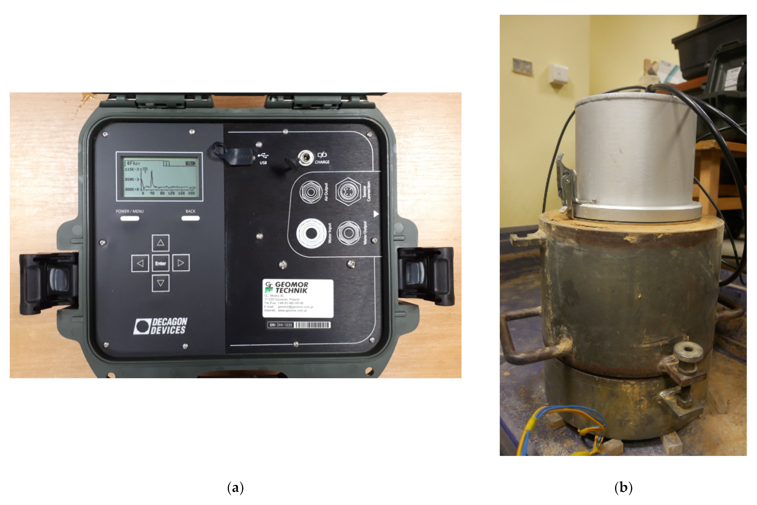
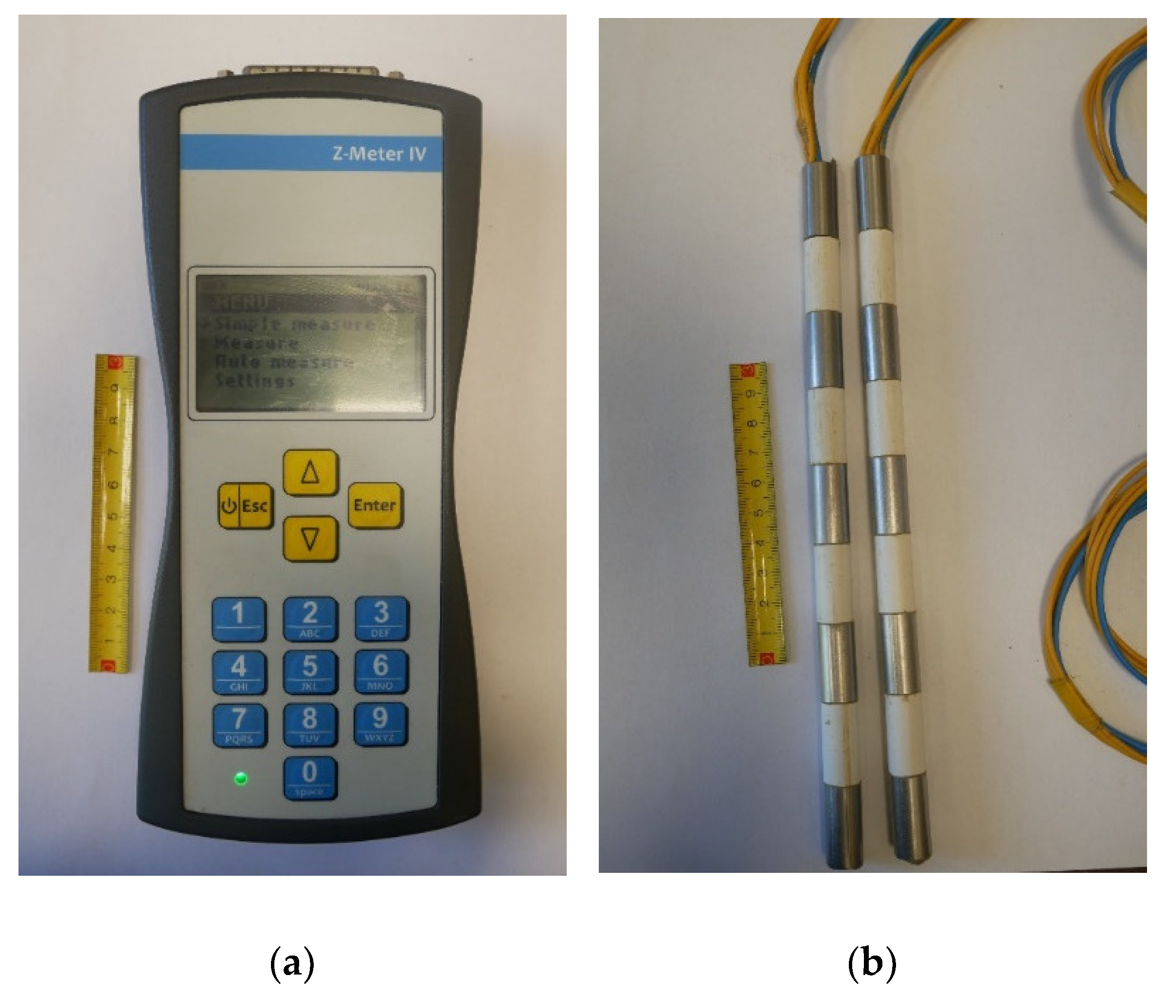
2.3. Monitoring of the Infiltration Process Using the EIS Method

The EIS method used in this study was applied to measure the electrical characteristics of the soil in a complex form, i.e., the resistance Rx (electrical resistance) and reactance X in the frequency range of the supply signal. Resistance is the actual (active) resistance in an electrical circuit and is the so-called electrical resistance, which depends on the soil type and the water content in its pores. On the other hand, reactance is the imaginary part of the impedance. A nonzero value of reactance causes a phase shift (phase difference) between the intensity and voltage of the electric current in the circuit. Reactance characterizes the changes in the soil caused by variations in its grain size or porosity [65].

The resistance measurements of the soil built into the model were carried out with two five-channel EIS measuring electrodes with a total length of 22.5 cm (Figure 3b) at a signal frequency of 2050 Hz. The electrodes were placed in the central part of the sample with a spacing of 20 cm. The measuring electrodes were paired up to a measuring probe with five vertical measuring segments (channels), 2.5 cm high each (current-conducting sections), spaced vertically every 2.5 cm. Due to the height of the soil sample, four measurement channels were used in the experiment. A Z-Meter (GEOtest, Brno, Czech Republic) was used to record the electrical resistance of the soil embedded in the model during water infiltration (Figure 3a). The device uses a measurement method that consists of comparing the measured impedance Z with normal resistance Rx with a known value of electrical resistance. The measurement results were recorded in a Microsoft Excel spreadsheet.

2.4. Calculations of Overland and Subsurface Runoff with the Use of Models Taking into Account the Infiltration Process

The obtained results of overland and subsurface runoff measurements were compared with the results of calculations carried out using the one-dimensional Green–Ampt model and the two-dimensional soil model developed in the GeoStudio 2020 software (Seequent, a Bentley Company, Broomfield, CO, USA), in which the Richards [19] equation was adopted to calculate the flow of water in the soil:

$$\frac{\partial \theta }{\partial t}=\frac{\partial }{\partial x}\left[k_x\frac{\partial H}{\partial x}\right]+\frac{\partial }{\partial z}\left[k_z\frac{\partial H}{\partial z}\right]+Q,$$

(1)

where θ (-) is the volumetric water content, t (s) is time, k_x (m·s⁻¹) is the hydraulic conductivity of the soil in the x-direction, k_z (m·s⁻¹) is the hydraulic conductivity of the soil in the z-direction, H (m) is the water total head, and Q (m·s⁻¹) is the boundary flux.

The calculation of the infiltration by the Green–Ampt method [20] consists of determining the soil capacity rate (potential infiltration rate):

$$f=k_s·i=k_s·\frac{z_f+{\psi }_f+H_p}{z_f}\left[\mathrm{m}·{\mathrm{s}}^{-1}\right]$$

(2)

where k_s (m·s⁻¹) is the hydraulic conductivity of a soil, given as half of the value of the soil coefficient of permeability [66]; i (-) is the hydraulic gradient; H_p (m) is the height of ponding, often assumed to be equal to 0, because surface ponding triggers overland runoff; z_f (m) is the depth of the wetting front location; and ψ_f (m) is the weight of soil suction pressure at the base of the wetting front.

The height of the soil suction pressure at the base of the wetting front can be determined in various ways [3,67]. In this study, the formula given by Maidmend [3] was used, as shown in Equation (3):

$$\begin{gathered} {\psi }_f=0.01·\left[6.53-7.326·n+0.00158C{l}^2+3.809·n^2+0.000344·Sa·Cl-0.04989·Sa·n+0.0016 \\ ·S{a}^2·n^2+0.0016·C{l}^2·n^2-0.0000136·S{a}^2·Cl-0.00348·C{l}^2·n-0.000799·S{a}^2 \\ ·n\right] \left[\mathrm{cm}\right] \end{gathered}$$

(3)

where n (-) is the soil porosity, S_a (%) is the sand fraction content, and Cl (%) is the clay fraction content. The equation is easy to calculate and there is no need for information on the soil water characteristic curve (retention curve).

The above equation assumes that the value of the suction pressure at the base of the wetting front is independent of the soil moisture content. Therefore, for the purposes of the analyses, Equation (3) was modified to take into account the soil moisture content:

$${\psi }_{fm}=\left(1-S_r\right)·{\psi }_f [\mathrm{cm}],$$

(4)

where S_r (-) is the degree of soil saturation.

In the calculations, the infiltration capacity is compared with the intensity of precipitation, assuming that, until the values of both parameters are equal, the total amount of rainwater infiltrates the soil profile. This is referred to as the surface flooding time (t_p). After this, the overland runoff begins, and the amount of water accumulated (F) in the soil profile can be calculated from the following relationship:

$$F=F_p+k_s·\left(t-t_p\right)+\left({\theta }_s-{\theta }_i\right)·{\psi }_{fm}·ln\left|\frac{\left({\theta }_s-{\theta }_i\right)·{\psi }_{fm}+F}{\left({\theta }_s-{\theta }_i\right)·{\psi }_{fm}+F_p}\right|,$$

(5)

where F_p (mm) is the accumulation of rainwater in the soil at the moment of ponding of the soil surface, θ_s (-) is the soil moisture content at full saturation, and θ_i (-) is the soil moisture content before rainfall.

The solution to Equation (5) was found by using the iterative method in Microsoft Excel. The values of initial soil moisture before the first rainfall episode were determined on the basis of the soil porosity and mass moisture, while for the next two episodes the balance of water infiltrating the soil and the amount of overland and subsurface runoff were taken into consideration.

The second method of calculating overland runoff was based on numerical calculations using the physical Richards equation [19] of water flow in the zone of incomplete saturation. The calculations were conducted in the SEEP/W module (Seequent, a Bentley Company, Broomfield, CO, USA) for the two-dimensional model of the plot (Figure 4), assuming that the outflow of water from the ground occurs in the lower part of one of the walls. On the other hand, the amount of rainfall, its duration, and the periods between individual rainfall episodes were the same as in the actual studies. As a result of the calculations, the volume of water stored and drained from the soil was obtained, and the amount of overland runoff was calculated as the difference between the rainfall and the amount of water infiltrating the soil:

$$OF=R-S,$$

(6)

where OF (mm) is the overland runoff, R (mm) is the rainfall, and S (mm) is the height of the water column stored in the ground.

For the purpose of calculating the coefficient of permeability of soil, values of (2 ÷ 5) × 10⁻⁶ m·s⁻¹ were adopted from the Saturo infiltrometer tests, and the retention characteristics were determined using the retention parameters proposed by the SEEP/W program for silty soils.

2.5. Estimation of Overland and Subsurface Runoff Using the MSME Model

The concept of the model was introduced by Wałęga and Amatya [68] for a flat coastal watershed. The method is based on a common SCS-CN method used to calculate direct runoff. In the present study, the concept was slightly modified. In the MSME model, the direct runoff was estimated for every event using the following equations:

$$Q=\frac{\left(P-I_a\right)·\left(P-I_a+M\right)}{P-I_a+S} if P>I_a;$$

(7)

Supposing $Q=0$ then:

$$I_a=\lambda ·\left(S-M\right),$$

(8)

where S is the maximum retention capacity, and P (mm) is the sum of the precipitation during the event.

In Equation (7), the higher the antecedent moisture (M), the lower the initial abstraction (I_a), and vice versa. The antecedent moisture content is given as follows:

$$M=\beta \left[\frac{\left(P5-\lambda S\right)\lambda S}{\left(P5-\lambda S\right)+S}\right] for P5>S$$

(9)

$$M=0 for P5<S,$$

(10)

where β (-) and λ (-) are parameters that are optimized, and P5 is the amount of water that infiltrated during the previous five-day period.

Subsurface runoff (MSME_Qsubs) was calculated using the following equations:

$$MSM{E}_{Qsubs}=\frac{\left(P-I_{a1}\right)·\left(P-I_{a1}+M\right)}{\left(P-I_{a1}+S_a\right)} if P>I_{a1}$$

(11)

$$I_{a1}=a·\left(PET5+\left(S_a-M\right)\right)$$

(12)

$$MSM{E}_{Qsubs}=0 if P<I_{a1}$$

(13)

$$M=\beta ·\frac{\left(P5-PET5\right)·S_a}{\left(P5-PET5\right)+S_a}$$

(14)

$$S_a=a\left(\frac{25400}{CN}-254\right),$$

(15)

where I_a1 (mm) is the initial abstraction for subsurface runoff, PET5 (mm) is the sum of five days’ potential evapotranspiration computed using the Penman–Monteith method, S_a (mm) is the maximum potential retention for the area where subsurface runoff occurs, and a (-) is the coefficient for the proportion of area with saturated soil.

Overland runoff (MSME_Qsurf) was calculated using the following equations:

$$MSM{E}_{Qsurf}=\frac{\left(P-I_{a2}\right)·\left(P-I_{a2}\right)}{P-I_{a2}+S_b} if P>I_{a2}$$

(16)

$$I_{a2}=\left(1-a\right)·\left(PET5+S_b\right)$$

(17)

$$MSM{E}_{Qsurf}=0 if P<I_{a2}$$

(18)

$$S_b=\left(1-a\right)·\left(\frac{25400}{100-CN}-254\right),$$

(19)

where I_a2 (mm) is the initial abstraction for overland runoff, S_b (mm) is the maximum potential retention for the area where overland runoff occurs, and CN (-) is the curve number (CN) parameter.

Total runoff was calculated as the sum of overland and subsurface runoff:

$$MSM{E}_{tot}=MSM{E}_{Qsurf}+MSM{E}_{Qsubs}.$$

(20)

In the initial phase of rainfall, when the soil is dry with a large soil water deficit (storage), it is assumed that runoff does not occur. In the case of highly impermeable soil, after the first soil saturation threshold is exceeded, overland runoff begins. The factor determining the proportion of saturated area is parameter “a”, which is calibrated based on the observed rainfall and runoff from the laboratory model. If the soil is almost fully saturated ($S_r\cong 1.0$), subsurface runoff may occur after overland runoff because the wetting front is moving in the soil profile and saturation increases. If the rainfall continues, the soil will continue to be saturated, achieving the second threshold and resulting in subsurface runoff. To perform runoff calculations for these conditions, we assumed that the CN parameter from the original SCS-CN method can be used to test these hypotheses.

The calculations were carried out using the following procedure: in the first case, CN was determined for each of the rainfall–overland runoff events based on the equations given by Wałęga et al. [69] and parameters α, λ, and β were optimized using the Nash–Sutcliffe coefficient as an objective function. In addition, the results of depth of runoff were compared with the one-dimensional Green–Ampt model and two-dimensional Richards’ equation.

The root mean square error (RMSE) and the Nash–Sutcliffe modeling efficiency (EF) [70] were used as goodness-of-fit measures to assess and compare the performance of the models:

$$RMSE=\sqrt{\frac{1}{N}·{\displaystyle \sum }_{i=1}^N{\left(Q_{obs,i}-Q_{calc,i}\right)}^2}\left[-\right]$$

(21)

$$EF=1-\frac{{{\displaystyle \sum }}_{i=1}^N{\left(Q_{obs,i}-Q_{calc,i}\right)}^2}{{{\displaystyle \sum }}_{i=1}^N{\left(Q_{obs,i}-{\overline{Q}}_{obs,i}\right)}^2}-,$$

(22)

where Q_obs,i (mm) is the observed direct runoff, Q_calc,i (mm) is the calculated direct runoff, ${\overline{Q}}_{obs,i}$ (mm) is the mean value of the observed direct runoff values, and N (-) is the number of observations.

Equation (21) was used as an objective function during the calibration processes. Optimum values of these parameters were obtained when EF reached the maximum values. The calibration processes were performed using the Solver tool in Microsoft Excel, where a GRG nonlinear method was used.

Ritter and Muñoz-Carpena [71] criteria were used to evaluate the model performance, where EF < 0.65 was deemed the lower threshold for unsatisfactory performance. The other model performance ratings were as follows: acceptable (0.65 ≤ EF < 0.80), good (0.80 ≤ EF < 0.90), and very good (EF > 0.90).

Results of tests were visualized using the Python (Python Software Foundation License) libraries Matplotlib [72] and Seaborn [73], and prepared using Google Colaboratory (Google Research, Mountain View, CA, USA) notebook.

3. Results of Studies

3.1. Geotechnical Properties of Soil

In terms of geotechnical properties, the examined soil corresponded to multifraction coarse clay silt (clCSi). The particle size distribution was dominated by the silt fraction, the share of which was 73%; the sand fraction was 18.3%, the clay fraction 8.5%, and the gravel fraction 0.2% (Figure 5). The plasticity limit of the soil was 15.7%, and the liquid limit was 26.1%, which allowed us to conclude that the tested soil was in a compact state during the formation of the sample in the precipitation simulator. The study of compaction parameters showed that the maximum dry density of the soil was 1.83 g·cm⁻³ at the optimum moisture content of 13.4%.

The process of water infiltration into cohesive soil is limited, so the subsurface runoff formation will be slightly delayed. It should also be pointed out that, in the case of cohesive soils, internally bound water is very viscous, has low liquidity, and is not subject to gravity. Although water bound in the pores of cohesive soils makes up a significant part of the pore volume, it cannot generate and transmit the pressure of the pore water and cannot cause seepage [74]. Therefore, the determination of the coefficient of permeability for proper numerical modeling of overland and subsurface runoff is important.

The laboratory tests conducted on the soil permeability coefficient showed that its values decreased along with the increase of the compaction index from I_S = 0.88 to 0.99 (decreased porosity from 0.41 to 0.32), and ranged from 4.31 × 10⁻⁷ to 1.11 × 10⁻⁸ m·s⁻¹, respectively (Figure 6). On the other hand, the coarse clay silt coefficient of permeability determined with the Saturo infiltrometer (Figure 7), when the porosity value is 0.41, corresponding to the compaction index of I_S = 0.88, was on average 4.92 × 10⁻⁶ m·s⁻¹. The obtained values indicate that the tested soil may be classified as poorly or semipermeable [75].

The comparison of the value of the filtration coefficient at the compaction index I_S = 0.88, obtained from the oedometer and infiltrometer tests, showed that the oedometer value was an order of magnitude lower than that obtained from the infiltrometer tests. These differences may be due to the size of the samples and the test method. Taking into account the different values of the coefficient of permeability (filtration), calculations of the overland and subsurface runoff were conducted for four values of this coefficient. One of them (the lowest) was the average value of the oedometer tests for the sample with a compaction index of I_S = 0.88, so the porosity was n = 0.40 (k = 5.0 × 10⁻⁷ m·s⁻¹). The next two values (k = 4.0 × 10⁻⁶ and 2.0 × 10⁻⁶ m·s⁻¹) were adopted from the Saturo infiltrometer tests. These values corresponded to the range of values of the infiltration rate when tests were approaching the end. The last value of the coefficient of permeability (k = 1.0 × 10⁻⁶ m·s⁻¹) was adopted as a geometric mean of the parameter derived from the two methods used.

3.2. Overland and Subsurface Runoff

Table 1. Test conditions in the precipitation simulator.

Runoff Slope (%)	Rainfall Episode	Precipitation			Soil Moisture Content (1) before Rainfall (%)	Volumetric Soil Moisture Content (2) before/after the Examination (-)	Runoff Record
		Height (mm)	Duration (min)	Intensity (mm·min−1)			Overland	Subsurface
2.5	1	30	40	0.75	10.0	0.39/0.72	yes	no
	2				24.2	0.72/0.92	yes	yes
	3				26.4	0.81/0.94	yes	yes
5.0	1				10.0	0.39/0.71	yes	no
	2				21.5	0.71/0.90	yes	no
	3				23.0	0.87/0.97	yes	yes

⁽¹⁾ value from the examination, ⁽²⁾ value calculated from the water balance.

summarizes the scope of the conducted tests and their preliminary results, together with the observations of overland and subsurface runoff formation. The test results obtained for both runoff slopes indicate a similar trend of changes in the overland and subsurface runoff values. Generally, the lowest values of runoff were observed during the first rainfall episode, while the highestwas seen in the last (third) episode. It was also noticeable that the subsurface runoff did not occur in the first rainfall episode.

The values of overland runoff obtained in the first rainfall episode, with an initial soil moisture content of about 10%, were small and appeared in the final period of rainfall. The maximum overland runoff intensity, in the case of the model with a 2.5% soil surface slope inclination, occurred in the 40th minute, while in the case of a 5.0% slope it occurred in the 38th minute (Figure 8). This value, in the case of the model with a higher inclination of the soil surface, was more than twice as high as for the smaller inclination. These values corresponded to an overland runoff intensity of 0.08 and 0.2 mm·min⁻¹ for slopes of 2.5 and 5.0%, respectively. For this rainfall episode, no subsurface runoff was observed (Figure 9). Before the research started, the soil was characterized by a relatively low moisture content, and therefore also a high value of moisture content deficit and, at the same time, high capacity. As a result of rainfall, most of the moisture was retained in the soil, increasing its moisture content before the next rainfall event. This was confirmed by the soil moisture content measurement results, determined before the second rainfall episode, which increased by 2.5- and 2.2-fold for runoff surface slopes of 2.5 and 5.0%, respectively (Table 1). The results of the degree of soil saturation (the ratio of water volume in the soil to the pore volume) calculations indicate that it increased from 0.39 to 0.71–0.72 after the first rainfall episode. Theoretical calculations of soil moisture content showed that the maximum moisture content of soil is 26.1%, and the results of determinations of this parameter in the subsurface part of the soil sample showed that the degree of saturation was slightly higher (0.82–0.93).

In the second and third rainfall episodes, the overland runoff appeared quite quickly, between the 5th and 8th minutes of the experiment (Figure 8). The maximum values of the runoff intensity were 0.44 and 0.43 mm·min⁻¹ in the second rainfall episode and 0.58 and 0.68 mm·min⁻¹ in the third episode, for a runoff surface slope of 2.5 and 5.0%, respectively. It is noticeable that the maximum values of the runoff intensity in the third rainfall episode were slightly lower than the rainfall intensity (0.75 mm·min⁻¹).

The results of measurements of the subsurface runoff (Figure 9) showed that it did not occur during the first rainfall episodes for both inclinations of the soil surface. With an inclination of the soil surface of 2.5%, the maximum values of the subsurface runoff in the second and third rainfall episodes were similar—0.01 mm·min⁻¹. It should, however, be noted that, in the case of the second rainfall episode, the subsurface runoff occurred only after the end of the rainfall. In the case of the model with a 5.0% slope, subsurface runoff was observed only in the third rainfall episode. At the peak, its intensity was twice as high as that measured for the runoff in the model with a lower inclination of the soil surface and was 0.025 mm·min⁻¹. Lack of subsurface runoff in the first episode at both slopes may result from the lowest initial soil moisture, which in the case of cohesive soils means that rainfall reaching the soil surface does not seep but forms a layer of flowing water. This is related to the aggregation of soil particles and clogging of its pores. Laboratory studies by Morbidelli et al. [76] led to similar conclusions, i.e., that in sloping bare soils, overland runoff is formed even when the rainfall intensity is smaller than the saturated hydraulic conductivity.

The results of measurements of soil moisture before the second and third rainfall episodes (Table 1) showed an increase in the moisture content. The calculations of the soil moisture content also indicate the influence of subsequent rainfall episodes on the change in the degree of saturation of the soil pores with water. It should be noted, however, that the maximum values of this parameter indicate that the soil was not fully saturated. On the other hand, the flow of water through the soil (from top to bottom) may cause the closure of air bubbles in the soil pores and thus an actual reduction in the retention capacity of soil. This phenomenon will certainly accelerate the process of overland runoff formation.

The values of cumulative runoff in each of the measurement cycles for both soil surface inclinations after 40 min of rainfall (when it stopped) were slightly higher for the model with a higher soil surface inclination.

In the first measurement cycle, the value of the cumulative runoff at the end of the rainfall was 0.48 and 1.79 mm for a soil surface inclination of 2.5 and 5.0%, respectively. However, in the second measurement cycle, after 40 min of rainfall, the runoff was on average 12.9 and 13.2 mm for a runoff surface inclination of 2.5 and 5.0%, respectively. After the third measurement cycle, the cumulative runoff at the end of the rainfall was 19.0 and 21.2 mm, and after 40 min it was 18.9 and 21.4 mm, respectively, for a model with a surface inclination of 2.5 and 5.0%. However, it should be noted that, after the rainfall stopped, the overland runoff was still recorded, and it was highest after the end of the third rainfall episode. In total, it amounted to 25.2 and 26.8 mm for models with a surface inclination of 2.5 and 5.0%, respectively.

The cumulative subsurface runoff was small compared to the overland runoff and, in the case of the model with a surface inclination of 2.5%, it was 0.4 and 0.7 mm, respectively, after the second and third rainfall episodes. On the other hand, for the model with a 5.0% inclination, it did not exceed 1.4 mm after the third rainfall episode.

The presented research results indicate that the values of overland runoff for both inclinations of soil surface were slightly higher than the values obtained for the higher soil surface inclination. During the study, it was also observed that, with a smaller runoff surface slope, the energy of the falling rain caused a splash of the soil, which significantly reduced the water infiltration into the soil, destroying its structure and reducing its permeability [77,78]. This phenomenon was observed to a much lesser extent in the case of a 5.0% inclination of the soil surface.

3.3. Monitoring of Water Infiltration within the Soil

One way to control soil water flow is measuring the linear electrical response of a porous material excited by a weak electromagnetic signal over a wide frequency range. This method allows us to control the groundwater or infiltration water flow, as well as to identify nonhomogeneous areas in terms of soil porosity [79]. The values of electrical resistance depend on the temperature of water and soil, the air and soil moisture content, and the atmospheric pressure [80,81].

This experiment was conducted using a probe with four measuring channels, the vertical spacing of which was 2.5 cm. The results indicate a change in the soil resistance over time, resulting from water infiltration into the soil during rainfall episodes (Figure 10 and Figure 11). It is notable that, along with the duration of the experiment, in subsequent rainfall episodes, the value and range of the electrical resistance of the soil clearly decreased because the soil moisture increased. In the case of the model with an inclination of 2.5% (Figure 10), the greatest changes in the electrical resistance of the soil occurred during the first episode of rainfall, while before and during the third episode, the changes were insignificant, indicating a high degree of soil moisture. On the other hand, in the case of the model with a 5.0% inclination (Figure 11), in the first and third rainfall episodes, noticeable changes in the electrical resistance of the soil were found, and in the second episode, apart from the lowest measuring channel, no significant changes in the electrical resistance of the soil were observed. This indicates that the first rainfall episode caused fundamental changes in the degree of soil moisture content in the upper soil layer, while the second episode caused only a shift of the wetting front to the lower part of the soil. It is also noticeable that, in the initial period of the third rainfall episode there was a significant decrease in the soil resistance, and the values recorded after the end of the experiment were similar to the values in the final part of the experiment for the model with a lower soil surface inclination. It can be noted that, for both runoff surface inclinations, the lowest values of soil resistance were recorded in the lower part of the soil sample, and the highestin the upper part, which may indicate that the soil moisture content increases with depth. This relationship may also be an indicator of the formation of subsurface runoff, which appeared in the third rainfall episode at a 5% inclination of the soil surface. On the other hand, in the case of the 2.5% inclination of the soil surface, the resistance values in the lower part of the soil sample were relatively constant in the second episode and subsurface runoff was recorded immediately after the end of this episode. The results of soil resistance tests indicate a change in soil moisture content and provide the basis for further research on the use of soil resistance to monitor the rate of water infiltration.

3.4. Verification of Calculation Models

3.4.1. Green–Ampt and Richards Models

The research results confirmed the effect of individual rainfall episodes on the amount of overland runoff generated. For comparison, theoretical calculations of water infiltration were carried out using two calculation methods, taking into account the physical properties of the soil (

Table 2. Summary of measurement and calculation results for overland and subsurface runoff.

Number of the Rainfall Episode	Type of Runoff	Soil Coefficient of Permeability Used in the Calculations (m·s−1)	Inclination of Soil Surface
			2.5%			5.0%
			Observations	Model		Observations	Model
				Green–Ampt	Richards		Green–Ampt	Richards
			Runoff Value (mm)
1	overland	4.0 × 10−6 2.0 × 10−6 1.0 × 10−6 5.0 × 10−7	0.61	0.00 3.02 9.76 15.49	0.96 1.32 6.85 12.96	2.03	0.00 3.02 9.76 15.49	0.20 0.88 6.76 12.91
	subsurface	4.0 × 10−6 2.0 × 10−6 1.0 × 10−6 5.0 × 10-7	0.00	-	0.00 0.00 0.00 0.00	0.0	-	0.00 0.00 0.00 0.00
2	overland	4.0 × 10−6 2.0 × 10−6 1.0 × 10−6 5.0 × 10−7	16.11	6.83 14.24 19.37 22.78	7.38 8.33 14.46 19.32	14.15	6.10 13.59 18.87 22.41	8.25 8.95 15.27 19.91
	subsurface	4.0 × 10−6 2.0 × 10−6 1.0 × 10−6 5.0 × 10−7	0.39	-	0.19 0.00 0.00 0.00	0.0	-	0.56 0.19 0.00 0.00
3	overland	4.0 × 10−6 2.0 × 10−6 1.0 × 10−6 5.0 × 10−7	25.17	11.23 17.94 22.14 24.78	28.25 28.36 18.14 18.01	26.78	14.61 20.60 24.10 26.20	28.11 28.31 17.88 18.00
	subsurface	4.0 × 10−6 2.0 × 10−6 1.0 × 10−6 5.0 × 10−7	0.75	-	0.90 0.77 0.00 0.00	1.53	-	1.42 0.77 0.00 0.00
Total	overland	4.0 × 10−6 2.0 × 10−6 1.0 × 10−6 5.0 × 10−7	43.72	18.1 35.2 51.3 63.1	36.59 38.00 39.46 50.29	42.96	20.71 37.21 52.73 64.10	36.56 38.14 39.91 50.82
	subsurface	4.0 × 10−6 2.0 × 10−6 1.0 × 10−6 5.0 × 10−7	5.20	-	1.49 0.91 0.00 0.00	2.66	-	2.42 0.78 0.00 0.00

). The results of the calculations show a significant influence of the coefficient of permeability on the results of the overland and subsurface runoff calculations. Generally, for lower values of the coefficient of permeability, higher values of overland runoff and lower values of subsurface runoff were obtained. The exemplary results of overland runoff calculations using the Green–Ampt method (Figure 12) indicate that the greatest discrepancies between the calculation and observation results were obtained in the first rainfall episode, where the calculated overland runoff value was significantly greater than the calculated value. The root mean square error and the Nash–Sutcliffe coefficient showed that, in the case of overland runoff calculations, the most accurate values of both parameters were obtained with a permeability coefficient of 2.10 × 10⁻⁶ m·s⁻¹. The value of the EF parameter (

Table 3. Values of metrics—RMSE and Nash–Sutcliffe EF [70].

Type of Runoff	Soil Coefficient of Permeability Used in the Calculations (m.s−1)	Inclination of Soil Surface
		2.5%		5.0%
		Model		Model
		Green–Ampt	Richards	Green–Ampt	Richards
Root Mean Square Error, RMSE (mm) (Equation (21))
overland	4.0 × 10−6 2.0 × 10−6 1.0 × 10−6 5.0 × 10−7	162.15 35.38 59.77 153.62	49.50 41.10 52.57 123.60	125.29 22.79 51.50 144.27	23.07 17.70 59.35 132.08
subsurface	4.0 × 10−6 2.0 × 10−6 1.0 × 10−6 5.0 × 10−7	-	0.25 0.30 0.63 0.63	-	0.19 0.33 1.35 1.35
Modeling efficiency, EF [-] (Equation (22))
overland	4.0 × 10−6 2.0 × 10−6 1.0 × 10−6 5.0 × 10−7	0.09 0.80 0.66 0.14	0.72 0.77 0.70 0.31	0.74 0.95 0.89 0.70	0.95 0.96 0.87 0.72
subsurface	4.0 × 10−6 2.0 × 10−6 1.0 × 10−6 5.0 × 10−7	-	−0.54 −0.86 −2.86 −2.86	-	0.79 0.64 −0.50 −0.50

) for the model with a 2.5% inclination was 0.77–0.80 in the Green–Ampt and Richards method, respectively, and 0.95–0.96 for the model with a 5.0% inclination of the ground surface. On the other hand, acceptable EF values (0.64–0.79) were obtained for the model with a surface inclination of 5% for the two highest values of the coefficient of permeability. This is taking into account that, in the analyzed cases, overland runoff dominated, so the results of the calculations were used for further analyses, with a coefficient of permeability of 2.10 × 10⁻⁶ m·s⁻¹.

Figure 13a and Figure 14a compare the results of numerical calculations of overland and subsurface runoff from the Richards model with the results of laboratory tests. The calculations were carried out as a single time series, which started at least ten minutes before the beginning of the first rainfall episode and ended several dozen minutes after the end of the last rainfall episode. The time intervals between the individual rainfall episodes were identical to those used in the laboratory experiments.

The calculation results for both inclinations of the runoff soil surface showed that the total values of overland and subsurface runoff were slightly lower than those obtained from the tests. It could be noticed that the overland runoff values calculated for the first rainfall episode were overestimated compared to those measured in laboratory conditions. On the other hand, the values calculated for the second rainfall episode were similar, while those for the third episode were underestimated compared to the results obtained from the measurements. In the case of the last rainfall episode, the measured overland runoff was 27 mm, representing almost 90% of the precipitation.

3.4.2. MSME Model (Verification of Suitability for the Total Runoff Estimation)

Table 4. Average runoff characteristics from the experimental laboratory model and MSME model.

Slope Inclination	Qsurfobs	Qsubsurfobs	Qtotobs	Qsurcalc	Qsubsurfcalc	Qtotcalc	CN	M	Sa	Sb	Ia1	Ia2
-	mm				-				mm
2.5	10.8	0.40	11.16	11.19	0.21	11.40	89.7	0.00	27.1	787.1	22.9	122.6
5.0	12.1	0.47	12.53	11.91	0.59	12.51	93.0	0.00	18.2	654.7	16.5	62.2

Notes: Q_surfobs is the observed overland runoff, Q_subsurfobs is the observed subsurface runoff, Q_totobs is the observed total runoff (sum of overland and subsurface runoff), Q_surfcalc is the calculated observed overland runoff, Q_subsurfcal is the calculated observed subsurface runoff, Q_totcalc is the calculated total runoff (sum of overland and subsurface runoff), I_a1 is the initial abstraction for subsurface runoff, M is the antecedent moisture content, S_a is the maximum potential retention for the area where subsurface runoff occurs, I_a2 is the initial abstraction for overland runoff (in mm), S_b is the maximum potential retention for the area where overland runoff occurs (mm), and CN is the calculated curve number.

shows the mean values of the overland and subsurface runoff obtained based on the results of laboratory tests and calculations using the MSME model. The test results showed that the subsurface runoff in the tested soil was small and constituted just over 3.3% and 3.7% of the total runoff for the 2.5% and 5.0% soil surface inclination, respectively. The amount of overland and subsurface runoff from both the observation and the MSME model increased with the inclination of the runoff surface, which is consistent with the study of Chen et al. [26]. The results obtained from the MSME model were similar to the observations, regardless of the slope of the runoff surface. The RMSE error value was 0.52 and 0.05 mm for the 2.5% and 5.0% slope, respectively, while the EF coefficient was 0.99 in both cases. Therefore, it can be concluded that the MSME model allowed for a very good estimation of the total runoff, which proves the correct concept of runoff formation described by this model. The inclination of the runoff surface affects the soil degree of saturation, expressed by the parameter “a”, which for the 2.5% inclination of the runoff surface was 0.84, while for 5.0% it was 0.90. Thus, in the case of a surface with higher inclination, the subsurface runoff may be formed at a higher soil saturation. However, the differences in soil moisture content are small due to the fact that, during heavy rainfall, the infiltration rate depends on the runoff surface slope under conditions where it exceeds 10° [26]. The value of the CN parameter, understood as the catchment’s potential for runoff formation, is as high as 89.7 for a 2.5% surface slope and 93.0 for a 5% slope, which is understandable as the investigated land is characterized by a low infiltration capacity. At the same time, it should be noted that the inclination of the runoff surface affects the value of the CN parameter. The value of the M parameter related to the initial water content in the soil profile, coming from the infiltration of rainwater before the runoff occurred, is 0.00 for both variants of the runoff surface slope. This is caused by the methodology used to prepare the soil for testing, which is characterized by a relatively low moisture content. The values of S_a and S_b retention parameters were significantly lower for soil with a 5.0% slope in comparison to a 2.5% slope. It is related, as in the case of the CN parameter, to a lower water retention capacity in soils with a higher slope of the runoff surface, which was confirmed in this study. As a consequence, the initial losses of I_a1 parameter for subsurface runoff and I_a2 parameter for overland runoff were also reduced.

3.5. Discussion

When analyzing the influence of the surface inclination on the measured values of overland runoff, it can be concluded that it was not very significant. These results are consistent with the results of the analyses by Chen and Young [26], who showed that, at soil inclinations smaller than 10°, the differences in the amount of water infiltrating the soil are small, so the values of overland runoff will be similar. Similar results were generated in the field tests conducted by Smolska [32]. Laboratory tests carried out by Wang et al. [16] provide slightly different relationships, as they indicate that there are differences between the measured values of effective precipitation and the amount of water infiltrating the soil for surface inclinations of 3° and 5°. In general, the amount of overland runoff increases with increasing surface inclination, while the amount of water infiltrating the soil decreases. Unfortunately, Wang et al. [16] do not provide the physical properties of the soil they examined.

Interesting data were generated by numerical calculation. The results of soil degree of saturation calculations (Figure 13b and Figure 14b) indicate that, during the first rainfall episode, there were significant changes in the surface part of the soil sample, regardless of the soil slope. In the lower part of the sample, at a depth of 15.5 cm, these changes were very small and appeared at the end of the precipitation event. This seems to be consistent with the results of measurements of the electrical resistance of the soil (Figure 10 and Figure 11). The results of calculations of soil moisture content in the upper part of the soil sample indicate that, in the final phase of the first episode, the soil becomes saturated, which coincides with the beginning of the overland runoff. This relationship indicates that the water flow in the soil is consistent with the assumptions of infiltration calculations using piston models, in which the wetting front formed in the upper part of the profile moves downwards with the existing water supply (precipitation) to the soil.

In the second rainfall episode, the saturation of the surface layer of soil occurred in the initial period of the rainfall, similar to when the overland runoff began. On the other hand, the soil moisture content in the lower part of the soil sample systematically increases until soil saturation was achieved, at the end of the rainfall episode. The calculations show that, after the episode ends, the subsurface runoff starts, which is consistent with the test results obtained for the model with a runoff slope of 2.5%. The values resulting from the electrical resistance measurements in the lower part of the sample with a slope of 2.5% decreased noticeably at the end of this episode, to a value that was maintained until the end of the study. This dependence may indicate the saturation of the lower part of the sample. In the case of the soil sample with a 5.0% slope, the resistance value systematically decreased, but the minimum value was achieved only during the last rainfall episode.

The numerical calculations indicate that, after the second rainfall episode, the soil was fully or nearly saturated in virtually the entire sample profile. Therefore, during the third episode, most of the rainfall was transformed into overland runoff. When analyzing the results of the numerical calculations, it can be noticed that, before the beginning of the rainfall, the lower part of the sample was characterized by a higher moisture content than its upper part. This observation seems to be consistent with the results of soil resistance measurements, in which higher resistance values as well as lower soil moisture content were recorded closer to the surface. The numerical calculations indicate that, in the third rainfall episode, the infiltration of rainwater does not have the nature of a piston movement, but causes the supply of water to the lower, saturated zone of the soil.

It should also be noted that, in the third episode, both the measured and calculated values of the subsurface runoff were higher than in previous episodes. On the other hand, the calculated values of subsurface runoff were clearly smaller than the measured results. It seems that the differences may be significantly influenced by the accuracy of the preparation of the soil sample in the critical places, i.e., where the soil is exposed by the grooves capturing the water flowing out of the soil.

The numerical calculation of infiltration and overland runoff, which were simulated for laboratory runoff apparatus, was presented by Mendes et al. [34]. Analysis results indicate that the initiation of runoff generation is significantly related to the saturation of the soil sample in its upper part. They also stated that the simulated runoff results are insensitive to the length of the sample length, which differs from some site measurement results (e.g., [29,30,82]), which found that higher runoff coefficients were found on small plots than on large plots.

The results of the experiments conducted indicate that, during the rainfall, the amount of overland runoff for the model with a soil surface inclination of 5.0% was slightly higher. On the other hand, the total amount of rainfall was similar (Table 2). These results may prove the influence of the soil surface inclination on the delay in the outflow of water from the catchment, as confirmed by Wang et al. [16].

The obtained results also prove the significant influence of the soil moisture content on the conditions of formation and the amount of overland and subsurface runoff. The occurrence of a series of short-term and intense rainfall episodes favors an increase in the soil moisture content and a reduction in its retention capacity. Similar relationships are observed in natural conditions (e.g., [36,48]) and when taking into account the climate change observed over many years, e.g., short and intense rainfall in Central Europe [83] and other regions [84,85]. They generate overland runoff, often causing flooding, usually of a local nature. The conducted experiments showed that in extreme cases more than two-thirds of rainfall is transformed into overland runoff. Similar dependencies in natural conditions are presented, among others, by Kijowska-Strugała and Kiska [79], Scherrer et al. [36], and Zydroń et al. [86]. It should be emphasized that the formation of this process is greatly influenced by the soil permeability coefficient, and, in built-up areas, by the degree of surface sealing. In the presented studies, the precipitation intensity was, on average, 0.75 mm·min⁻¹, and the value of the coefficient of permeability was estimated at 0.12 mm·min⁻¹. In the case of less permeable soil, one should expect a higher value of overland runoff.

It should be noted that the results of laboratory tests concerned soil without vegetation cover, which may correspond to areas covered by construction work or ground communication routes. Similar conditions may also apply to bare soil. Measurements on bare soil [31,32] indicate that overland runoff on this kind of surface is higher than that on cultivated land or soil with vegetation cover. The research carried out by Mounirou et al. [43] showed the effect of land use and land cover changes on the water cycle in a small Sahelian watershed. Simulation results provided an explanation of the Sahelian area paradox. The authors proved that a change in the sealing of the catchment area could lead to an increase in surface runoff despite the drop in rainfall.

Results of runoff from the Green–Ampt and Richards equations were compared with the hydrological model MSME. The quality of the MSME model, despite its considerable simplicity compared to the physical models, was better than that of the Richards and Green–Ampt models. Therefore, the MSME model correctly describes the total runoff and its individual parts in the case of low-permeable soils. In the MSME model, the soil degree of saturation parameter “a” plays an essential role in separating subsurface and overland runoff. The value of the “a” parameter depends on the soil inclination. The values for the “a” parameter obtained in this study were much lower compared to in forest catchments with gentle slopes, as described by Wałęga et al. [13]. However, it should be taken into consideration that, in the case of a forest catchment, midsoil runoff is predominant, while overland runoff is formed only after very intense rainfall.

In the original methodology [4], the runoff surface slope is not taken into account in the calculation of the CN parameter; however, as the slope of the runoff surface increases, the runoff rate increases, and therefore the infiltration capacity decreases. A similar tendency was observed in the present study, i.e., that the water infiltration capacity was reduced with an increase in the runoff surface inclination. This was manifested by an increase in the value of the CN parameter. The impact of an increase in the inclination of the runoff surface on the value of the CN parameter has been the subject of many studies. For example, Młyński [87] showed that taking into account the slope of a catchment area improves the quality of adjusting the CN to the observed values.

The obtained results may be a good indicator of areas subject to high human pressure. The obtained results indicate that high-intensity overland runoff is accompanied by soil denudation processes, and therefore, in order to reduce the intensity of these processes, it seems reasonable to use appropriate biogeotechnical treatments.

4. Conclusions

Based on the results of tests conducted on the coarse clay silt, it can be concluded that overland runoff is the dominant type of runoff in the analyzed soil. The impact of subsurface runoff on the water balance will be small due to the low water permeability of the examined soil. This may have a significant impact on the formation of a flood wave in a watercourse in areas where there are soils with similar geotechnical characteristics, in particular in terms of filtration. Our tests proved that an increase in the soil surface inclination from 2.5% to 5.0% did not cause a significant change in the amount of overland runoff. However, increased dynamics of its formation was found, which was certainly influenced by the lack of a vegetation cover that would reduce and delay its formation.

The obtained results indicate that, at a low initial soil moisture content, the runoff is of Horton overland flow character, in which the subsurface layer of soil is mostly saturated, and in the case of high moisture content it is caused by the saturation of the entire soil profile. This is confirmed by the results of electrical resistance measurements and numerical calculations. It was demonstrated that intensive rainfall repeating in short intervals will contribute to the generation of significant overland runoff, and in extreme cases more than two-thirds of rainfall can be transposed into overland runoff.

It was also demonstrated that the Green–Ampt and Richards models correctly describe the course of the infiltration process and overland runoff formation. The Richards model, however, tended to underestimate the amount of subsurface runoff. The filtration coefficient adopted for the calculations has a very significant influence on the results of the calculations, especially in the case of the Green–Ampt model.

The MSME model can be used to estimate the overland runoff (Q_surf) and subsurface runoff (Q_subsr) of impermeable soils, and its quality is comparable to that of the Green–Ampt and Richards models. The Green–Ampt and Richards method are based on physical assumptions and soil properties, but the simple empirical model MSME has parameters that are optimized based on observed rainfall–runoff events. This may be the main reason why the results of the MSME model are slightly better than those achieved by physical approaches. A limitation of the MMSE model in relation to the physical models is the inability to determine the course of infiltration over time and the need to calibrate the parameters based on the observed rainfall–runoff episodes. However, since it is a simple empirical model, it can be used by hydrologists to estimate the runoff in catchments. So, it is necessary to conduct further research on the application of this model on a real scale in various catchments to prove its usefulness in engineering calculations. Also, the authors will consider performing a study on the influence of artificial drainage on runoff formation and would include these results in the analyzed models. In a real catchment, the use of modern technique, like satellite imagines will be considered to indirectly assess soil moisture and link them with the parameters of the MSME model.

References

1. Egiazarova, D.; Kordzakhia, M.; Wałęga, A.; Drożdżal, E.; Milczarek, M.; Radecka, A. Application of Polish experience in the implementation of the flood directive in Georgia—Hydrological calculations. Acta Sci. Pol. Form. Circumiectus 2017, 16, 89–110. [Google Scholar] [CrossRef]
2. Gądek, W.; Bodziony, M. The hydrological model and formula for determining the hypothetical flood wave volume in non-gauged basins. Meteorol. Hydrol. Water Manag. 2015, 3, 3–10. [Google Scholar] [CrossRef] [Green Version]
3. Maidmend, D.R. Handbook of Hydrology; CRC Press: Boca Raton, FL, USA, 1993. [Google Scholar]
4. USDA Natural Resources Conservation Service. Hydrology. In National Engineering Handbook; Chapter 10; USDA Soil Conservation Service: Washington, DC, USA, 2004. [Google Scholar]
5. Karabová, B.; Sikorska, A.; Banasik, K.; Kohnová, S. Parameters determination of a conceptual rainfall-runoff model for a small catchment in Carpathians. Ann. Wars. Univ. Life Sci.-SGGW. Land Reclam. 2012, 44, 155–162. [Google Scholar] [CrossRef]
6. Młyński, D.; Wałega, A.; Książek, L.; Florek, J.; Petroselli, A. Possibility of using selected rainfall-runoff models for determining the design hydrograph in mountainous catchments: A case study in poland. Water 2020, 12, 1450. [Google Scholar] [CrossRef]
7. Grimaldi, S.; Petroselli, A. Do we still need the rational formula? An alternative empirical procedure for peak discharge estimation in small and ungauged basins. Hydrol. Sci. J. 2015, 60, 67–77. [Google Scholar] [CrossRef]
8. Piscopia, R.; Petroselli, A.; Grimaldi, S. A software package for the prediction of design flood hydrograph in small and ungauged basins. J. Agric. Eng. 2015, 432, 74–84. [Google Scholar] [CrossRef] [Green Version]
9. Petroselli, A.; Grimaldi, S. Design hydrograph estimation in small and fully ungauged basin: A preliminary assessment of the EBA4SUB framework. J. Flood Risk Manag. 2018, 11, 197–201. [Google Scholar] [CrossRef]
10. Petroselli, A.; Grimaldi, S.; Piscopia, R.; Tauro, F. Design hydrograph estimation in small and ungauged basins: A comparative assessment of event based (EBA4SUB) and continuous (cosmo4sub) modelling approaches. Acta Sci. Pol. Form. Circumiectus 2019, 18, 113–124. [Google Scholar] [CrossRef]
11. Szymczak, T.; Krężałek, K. Prognostic model of total runoff and its components from a partially urbanized small lowland catchment. Acta Sci. Pol. Form. Circumiectus 2018, 18, 185–203. [Google Scholar] [CrossRef]
12. Yuan, Y.; Mitchell, J.K.; Hirschi, M.C.; Cooke, R.A. Modified SCS curve number method for predicting subsurface drainage flow. Trans. ASAE 2001, 44, 1673–1682. [Google Scholar] [CrossRef]
13. Wałęga, A.; Amatya, D.M.; Caldwell, P.; Marion, D.; Panda, S. Assessment of storm direct runoff and peak flow rates using improved SCS-CN models for selected forested watersheds in the Southeastern United States. J. Hydrol. Reg. Stud. 2020, 27, 100645. [Google Scholar] [CrossRef]
14. Sahu, R.K.; Mishra, S.K.; Eldho, T.I. Performance evaluation of modified versions of SCS curve number method for two watersheds of Maharashtra, India. ISH J. Hydraul. Eng. 2012, 18, 27–36. [Google Scholar] [CrossRef]
15. De Lima, J.L.M.P.; Singh, V.P. Laboratory experiments on the influence of storm movement on overland flow. Phys. Chem. Earth 2003, 28, 277–282. [Google Scholar] [CrossRef] [Green Version]
16. Wang, A.; Jin, C.; Pei, J. A modified hortonian overland flow model based on laboratory experiments. Water Resour. Manag. 2006, 20, 181–192. [Google Scholar] [CrossRef]
17. Chu, X.; Padmanabhan, G.; Bogart, D. Microrelief-controlled overland flow generation: Laboratory and field experiments. Hindawi Publ. Corp. Appl. Environ. Soil Sci. 2015, 2015, 642952. [Google Scholar] [CrossRef] [Green Version]
18. Danino, D.; Svoray, T.; Thompson, S.; Cohen, A.; Crompton, O.; Volk, E.; Argaman, E.; Levi, A.; Cohen, Y.; Narkis, K.; et al. Quantifying shallow overland flow patterns under laboratory simulations using thermal and LiDAR imagery. Water Resour. Res. 2021, 57, e2020WR028857. [Google Scholar] [CrossRef]
19. Richards, L.A. Capillary conduction of liquids in porous mediums. Physics 1931, 1, 318–333. [Google Scholar] [CrossRef]
20. Green, W.H.; Ampt, G.A. Studies of soils physics I. The flow of air and water through soils. J. Agric. Sci. 1911, 4, 1–24. [Google Scholar]
21. Mein, R.G.; Larson, C.L. Modeling infiltration during a steady rain. Water Resour. Res. 1973, 9, 2, 384–394. [Google Scholar] [CrossRef] [Green Version]
22. Chow, V.T.; Maidment, D.R.; Mays, L.W. Applied Hydrology; McGraw-Hill Book Company: New York, NY, USA, 1988. [Google Scholar]
23. Chen, L.; Young, M.H. Green-Ampt infiltration model for sloping surfaces. Water Resour. Res. 2006, 42, W07420. [Google Scholar] [CrossRef]
24. Chormański, J.; Ignar, S.; Cabański, P. Zastosowanie modelu infiltracyjnego Green’a i Ampt’a oraz metod GIS do określania opadu efektywnego w modelowaniu opad-odpływ na przykładzie zlewni górnej wilgi. Zesz. Probl. Postępów Nauk. Rol. 2008, 532, 77–89. [Google Scholar]
25. Cho, S.E.; Lee, S.R. Evaluation of surficial stability for homogeneous slopes considering rainfall characteristics. J. Geotech. Geoenviron. Eng. 2002, 128, 756–763. [Google Scholar] [CrossRef]
26. Cho, S.E. Infiltration analysis to evaluate the surficial stability of two-layered slopes considering rainfall characteristics. Eng. Geol. 2009, 105, 32–43. [Google Scholar] [CrossRef]
27. Muntohar, A.S.; Liao, H.J. Analysis of rainfall-induced infinite slope failure during typhoon using a hydrological—Geotechnical model. Environ. Geol. 2009, 56, 1145–1159. [Google Scholar] [CrossRef]
28. Bochenek, W.; Gil, E. Water circulation, soil erosion and chemical denudation in flysh catchment area. (In Polish: Procesy obiegu wody, erozji gleb i denudacji chemicznej w zlewni Bystrzanki). Przegląd Nauk. Inż. Kształt. Sr. 2007, 16, 28–42. [Google Scholar]
29. Bochenek, W.; Gil, E. The diversity of overland flow and soil wash on experimental plots of different lengths (Szymbark, Low Beskidy Mts.) (In Polish: Zróżnicowanie spływu powierzchniowego i spłukiwania gleby na poletkach doświadczalnych o różnej długości (Szymbark, Beskid Niski)). Pr. Studia Geogr. 2010, 45, 265–278. [Google Scholar]
30. Martinez, G.; Weltz, M.; Pierson, F.B.; Spaeth, K.E.; Pachepsky, Y. Scale effects on runoff and soil erosion in rangelands: Observations and estimations with predictors of different availability. Catena 2017, 151, 161–173. [Google Scholar] [CrossRef]
31. Mounirou, L.A.; Zoure, C.O.; Yonaba, R.; Paturel, J.E.; Mahe, G.; Niang, D.; Yacouba, H.; Karambiri, H. Multi-scale analysis of runoff from a statistical perspective in a small Sahelian catchment under semi-arid climate. Arab. J. Geosci. 2020, 13, 154. [Google Scholar] [CrossRef]
32. Smolska, E. Runoff and soil erosion on sandy slope in the last-glacial area—Plots measurements (Suwałki Lake land, NE Poland. (in polish: Spływ wody i erozja gleby na piaszczystym stoku w obszarze młodoglacjalnym—Pomiary poletkowe (Pojezierze Suwalskie, Polska NE)). Pr. Studia Geogr. 2010, 45, 197–214. [Google Scholar]
33. Święchowicz, J. Slopewash on agricultural foothill slopes in hydrological years 2007–2008 in Łazy (Wiśnicz Foothills). (In Polish: Spłukiwanie gleby na użytkowanych rolniczo stokach pogórskich w latach hydrologicznych 2007–2008 w Łazach (Pogórze Wiśnickie)). Pr. Studia Geogr. 2010, 45, 243–263. [Google Scholar]
34. Mendes, T.A.; Gitirana, G.F.N.J.; Rebolledo, J.F.R.; Vaz, E.F.; da Luz, M.P. Numerical evaluation of laboratory apparatuses for the study of infiltration and runoff. Braz. J. Water Resour. 2020, 25, e37. [Google Scholar] [CrossRef]
35. Rahardjo, H.; Lee, T.T.; Leong, E.C.; Rezaur, R.B. Response of a residual soil slope to rainfall. Can. Geotech. J. 2005, 42, 340–351. [Google Scholar] [CrossRef]
36. Scherrer, S.; Naef, F.; Faeh, A.O.; Cordery, I. Formation of runoff at the hillslope scale during intense precipitation. Hydrol. Earth Syst. Sci. 2007, 11, 907–922. [Google Scholar] [CrossRef] [Green Version]
37. Poesen, J. The influence of slope angle on infiltration rate and Hortonian overland flow. Geomorphology 1984, 49, 117–131. [Google Scholar]
38. Nassif, S.H.; Wilson, E.M. The influence of slope and rain intensity on runoff and infiltration (L’influence de l’inclinaison de terrain et de l’intensitéde pluie sur l’écoulement et l’infiltration). Hydrol. Sci. J. 1975, 20, 539–553. [Google Scholar] [CrossRef]
39. Kowalczak, P.; Kundzewicz, Z.W. Water-related conflicts in urban areas in Poland. Hydrol. Sci. J. 2011, 56, 588–596. [Google Scholar] [CrossRef] [Green Version]
40. Skotnicki, M.; Sowiński, M. The influence of depression storage on runoff from impervious surface of urban catchment. Urban Water J. 2015, 12, 207–218. [Google Scholar] [CrossRef]
41. Jarosińska, E. Local flooding in the USA, Europe, and Poland—An overview of strategies and actions in face of climate change and urbanisation. Infrastruct. Ecol. Rural. Areas 2016, 3, 801–821. [Google Scholar] [CrossRef]
42. Walczykiewicz, T.; Skonieczna, M. Rainfall flooding in Urban areas in the context of geomorphological aspects. Geoseinces 2020, 10, 457. [Google Scholar] [CrossRef]
43. Yonaba, R.; Biaou, A.C.; Koïta, M.; Tazen, F.; Mounirou, L.A.; Zouré, C.O.; Queloz, P.; Karambiri, H.; Yacouba, H. A dynamic land use/land cover input helps in picturing the Sahelian paradox: Assessing variability and attribution of changes in surface runoff in a Sahelian watershed. Sci. Total Environ. 2021, 757. [Google Scholar] [CrossRef]
44. Starkel, L. Geomorphic hazards in the Polish Flysch Carpathians. Studia Geomorphol. Carpatho-Balc. 2006, 11, 7–19. [Google Scholar]
45. Bodziony, M.; Baziak, B. Heavy rain effects on the example of 1997 and 2005 floods in the Wielka Puszcza basin. (In Polish: Skutki deszczy nawalnych na przykładzie powodzi w zlewni rzeki Wielkiej Puszczy w latach 1997 i 2005). Czas. Tech. Sr. 2007, 2, 13–28. [Google Scholar]
46. Wałega, A.; Cupak, A.; Amatya, D.M.; Drożdżal, E. Comparison of direct outflow calculated by modified SCS-CN methods for mountainous and high land catchments in upper vistula basin, Poland and lowland catchment in South Carlina, USA. Acta Sci. Pol. Form. Circumiectus 2017, 16, 187–207. [Google Scholar] [CrossRef]
47. Szwagrzyk, M.; Kaim, D.; Price, B.; Wypych, A.; Grabska, E.; Kozak, J. Impact of forecasted land use changes on flood risk in the Polish Carpathians. Nat. Hazards 2018, 94, 227–240. [Google Scholar] [CrossRef] [Green Version]
48. Gil, E. Water Circulation and Wash Down on the Flysch Slopes Used fo r Fanningpurposes in 1980–1990 Years (Results of Investigation on Experimental Plots at ResearchStation of Institute of Geography and Spatial Organization Polish Academy of Sciences in Szymbark) (In Polish: Obieg Wody i Spłukiwanie na Fliszowych Stokach Użytkowanych Rolniczo w Latach 1980–1990 (Wyniki Badań Przeprowadzonych na Poletkach Doświadczalnych na Stacji Naukowej IGiPZ PAN w Szymbarku)); Zeszyty IGiPZ PAN: Warszawa, Poland, 1999. [Google Scholar]
49. Moeyersons, J.; Makanzu, F.M.; Imwangana; Dewitte, O. Site- and rainfall-specific runoff coefficients and critical rainfall for mega-gully development in Kinshasa (DR Congo). Nat. Hazards 2015, 79, S203–S233. [Google Scholar] [CrossRef]
50. Mahmoud, S.H.; Mohammad, F.S.; Alazba, A.A. Determination of potential runoff coefficient for Al-Baha Region, Saudi Arabia using GIS. Arab. J. Geosci. 2014, 7, 2041–2057. [Google Scholar] [CrossRef]
51. Rutkowski, J. Budowa geologiczna regionu Krakowa. Prz. Geol. 1989, 37, 302–308. [Google Scholar]
52. Wójcik, A.; Kamieniarz, S.; Wódka, M.; Biajgo, A.; Janeczek, A.; Walatek, M. Atlas Osuwisk Miasta Krakowa; Urząd Miasta: Kraków, Poland, 2019. [Google Scholar]
53. Rutkowski, J. Szczegółowa Mapa Geologiczna Polski, Arkusz 973—Kraków; Państwowy Instytut Geologiczny: Warszawa, Poland, 1989. [Google Scholar]
54. Kolasa, M. Geotechniczne Własności Lessów Okolic Krakowa; Wydawnictwa Geologiczne: Warszawa, Poland, 1963. [Google Scholar]
55. PN-EN ISO 14688-2:2018-05; Rozpoznanie i Badania Geotechniczne. Oznaczanie i Klasyfikowanie Gruntów. Część 2: Zasady klasyfikowania. Polski Komitet Normalizacyjny: Warszawa, Poland, 2018.
56. Ziernicka-Wojtaszek, A.; Kopcińska, J. Variation in atmospheric precipitation in Poland in the years 2001–2018. Atmosphere 2020, 11, 794. [Google Scholar] [CrossRef]
57. Institute of Meteorology and Water Management-National Research Institute (in Polish: Instytut Meteorologii i Gospodarki Wodnej—Państwowy Instutu Badawczy). Available online: https://danepubliczne.imgw.pl/#ostrzezenia-archiwalne (accessed on 16 February 2022).
58. PN-EN ISO 17892–4:2017-01; Rozpoznanie i Badania Geotechniczne. Badania Laboratoryjne Gruntów. Część 4: Badanie Uziarnienia Gruntów. Polski Komitet Normalizacyjny: Warszawa, Poland, 2017.
59. PN-EN ISO 17892-12:2018-08; Rozpoznanie i Badania Geotechniczne. Badania Laboratoryjne Gruntów. Część 12: Oznaczanie Granic Płynności i Plastyczności. Polski Komitet Normalizacyjny: Warszawa, Poland, 2018.
60. PN-EN 13286-2:2010; Mieszanki Niezwiązane i Związane Hydraulicznie. Część 2: Metody Badań Laboratoryjnych Gęstości na Sucho i Zawartości Wody. Zagęszczanie Metodą Proktora. Polski Komitet Normalizacyjny: Warszawa, Poland, 2010.
61. Kaczyński, R.R. Warunki Geologiczno-Inżynierski na Obszarze Polski; Państwowy Instytut Geologiczny: Warszawa, Poland, 2017. [Google Scholar]
62. Lambor, J. Hydrologia Inżynierska; Arkady: Warszawa, Poland, 1971. [Google Scholar]
63. PN-S-02204:1997; Drogi Samochodowe. Odwodnienie Dróg. Odwodnienie Dróg. Polski Komitet Normalizacyjny: Warszawa, Poland, 2018.
64. Ziemiański, M.; Ośródka, L. Wpływ Zmian Klimatu na Środowisko, Gospodarka Społeczeństwo; Seria Publikacji Naukowo-Badawczych IMGW-PIB: Warszawa, Poland, 2012. [Google Scholar]
65. Pařilková, J.; Gombos, M.; Talt, A.; Kandra, B. Calibration of Z-meter device for measurement of volumetric moisture of soils. In Proceedings of the Eureka 2009, 5th Working Session within the Frame of the International Program EUREKA, Project No.: E!3838. Research, Development and Processing of Computerized Measuring System of Soils Moisture with EIS Method, Brno, Czech Republic, 11–13 November 2009; pp. 21–31. [Google Scholar]
66. Morel-Seytoux, H.J.; Khanji, J. Derivation of an equation of infiltration. Water Resour. Res. 1974, 10, 795–800. [Google Scholar] [CrossRef]
67. Muntohar, A.S.; Liao, H.J. Rainfall infiltration: Infinite slope model for landslides triggering by rainstorm. Nat. Hazards 2010, 54, 967–984. [Google Scholar] [CrossRef]
68. Wałęga, A.; Amatya, D.M. Application of modified SME-CN method for predicting event runoff and peak discharge from a drained forest watershed on the North Carolina Atlantic Coastal Plain. Trans. ASABE 2020, 63, 275–288. [Google Scholar] [CrossRef]
69. Wałęga, A.; Rutkowska, A.; Grzebinoga, M. Direct runoff assessment using modified SME method in catchments in the upper vistula river basin. Acta Geophys. 2017, 65, 363–375. [Google Scholar] [CrossRef]
70. Nash, J.E.; Sutcliffe, J.V. River flow forecasting through conceptual models part I. A discussion of principles. J. Hydrol. 1970, 10, 282–290. [Google Scholar] [CrossRef]
71. Ritter, A.; Munoz-Carpena, R. Performance evaluation of hydrological models: Statistical significance for reducing subjectivity in goodness-of-fit assessments. J. Hydrol. 2013, 480, 33–45. [Google Scholar] [CrossRef]
72. Hunter, J.D. Matplotlib: A 2D graphics environment. Comput. Sci. Eng. 2007, 9, 90–95. [Google Scholar] [CrossRef]
73. Waskom, M.L. Seaborn: Statistical data visualization. Open J. 2021, 6, 3021. [Google Scholar] [CrossRef]
74. Zhang, X.; Li, M.-B.; Sun, Y.-Z.; Zhu, Y.-T.; Yang, Z.-H.; Tian, D.-H. Study on permeability coefficient of saturated cohesive soil based on fractal theory. In IOP Conference Series: Earth and Environmental Science; IOP Publishing: Bristol, UK, 2019; Volume 242, p. 062055. [Google Scholar] [CrossRef]
75. Pazdro, Z. Hydrogeologia Ogólna; Wydawnictwa Geologiczne: Warszawa, Poland, 1983. [Google Scholar]
76. Morbidelli, R.; Saltalippi, C.; Flammini, A.; Cifrodelli, M.; Corradini, C.; Govindaraju, R.S. Infiltration on sloping surfaces: Laboratory experimental evidence and implications for infiltration modelling. J. Hydrol. 2015, 523, 79–85. [Google Scholar] [CrossRef]
77. Fox, D.M.; Le Bissonnais, Y.; Bruand, A. The effect of ponding depth on infiltration in a crusted surface depression. Catena 1998, 32, 87–100. [Google Scholar] [CrossRef]
78. Kijowska-Strugała, M.; Kiszka, K. Assessment of the splash on the foothill slope (Flysch carpathians, bystrzanka catchment) (In Polish: Ocena wielkości rozbryzgu gleby na stoku pogórskim (Karpaty fliszowe, zlewnia Bystrzanki)). Ann. Univ. Mariae Curie-Skłodowska Lub.—Pol. 2014, 69, 79–95. [Google Scholar] [CrossRef]
79. Pařilková, J.; Pařilek, L. Monitoring of the earth-fill dam of the Hornice reservoir monitored by EIS. In Proceedings of the Eureka 2015 3rd Conference and Working Session within the Frame of the International Program EUREKA, Project No.: e!7614. A System of Monitoring of Selected Parameters of Porous Substances Using the EIS Method in a Wide Range of Applications, Jaromerice nad Rokytnou, Czech Republic, 15–16 October 2015; pp. 205–224. [Google Scholar]
80. Pařilková, J.; Pařilek, L. Monitoring of the earth dam of a water reservoir by the method of electrical impedance spectrometry. In Proceedings of the Eureka 2008, 4th Working Session within the Frame of the International Program EUREKA; Project No.: E!3838. Research, Development and Processing of Computerized Measuring System of Soils Moisture with EIS Method, Brno, Czech Republic, 18–19 September 2008; pp. 21–31. [Google Scholar]
81. Gruchot, A.; Zydroń, T.; Cholewa, M.; Koś, K. Using impedance spectroscopy method (EIS) to monitor filtration—Model tests. In Proceedings of the 4th Conference and Working Session within the Frame-Work of the International Programme EUREKA, Project No.: E!7614, Lednice, Czech Republic, 13–14 October 2016; pp. 82–90. [Google Scholar]
82. Mounirou, L.A.; Yonaba, R.; Koïta, M.; Paturel, J.E.; Mahé, G.; Yacouba, H.; Karambiri, H. Hydrologic similarity: Dimensionless runoff indices across scales in a semi-arid catchment. J. Arid. Environ. 2021, 193, 104590. [Google Scholar] [CrossRef]
83. Bochenek, W. Evaluation of precipitation at the IG&SO pas research station in Szymbark during 40-year period (1971–2010) and its impact on the variability of water runoff from the Bystrzanka stream basin. (In Polish: Ocena zmian warunków opadowych na stacji naukowo-badawczej IGiPZ PAN W Szymbarku w okresie 40 lat obserwacji (1971–2010) i ich wpływ na zmienność odpływu wody ze zlewni Bystrzanki). Woda-Sr.-Obsz. Wiej. 2012, 12, 29–44. [Google Scholar]
84. Fratini, C.F.; Geldof, G.D.; Kluck, J.; Mikkelsen, P.S. Three points approach (3PA) for urban flood risk management: A tool to support climate change adaptation through transdisciplinarity and multifunctionality. Urban Water J. 2012, 9, 317–331. [Google Scholar] [CrossRef] [Green Version]
85. Le, T.T.A.; Lan-Anh, N.T.; Daskali, V.; Verbist, B.; Vu, K.C.; Anh, T.N.; Nguyen, Q.H.; Nguyen, V.G.; Willems, P. Urban flood hazard analysis in present and future climate after statistical downscaling: A case study in Ha Tinh city, Vietnam. Urban Water J. 2021, 18, 257–274. [Google Scholar] [CrossRef]
86. Zydroń, T.; Wałęga, A.; Bochenek, W. Application of selected hydrological models for the calculation of overland flow (In Polish: Zastosowanie wybranych modeli hydrologicznych do określania wielkości spływu powierzchniowego). Acta Sci. Pol. Form. Circumiectus 2014, 13, 81–93. [Google Scholar] [CrossRef]
87. Młyński, D. Analysis of problems related to the calculation of flood frequency using rainfall-runoff models: A case study in Poland. Sustainability 2020, 12, 7187. [Google Scholar] [CrossRef]
Figure 1. General view of Saturo infiltrometer (dual head) (a) and model of soil permeability testing by the infiltration method (b).
Sustainability 14 04962 g001
Figure 2. General view (a) and scheme (b) of the runoff simulator.
Sustainability 14 04962 g002
Figure 3. View of the Z-Meter IV apparatus (a) and measuring electrodes (b).
Sustainability 14 04962 g003
Figure 4. Cross section of the calculation model scheme (5.0% soil surface inclination).
Sustainability 14 04962 g004
Figure 5. The grain size distribution of the tested soil.
Sustainability 14 04962 g005
Figure 6. Changes in the coarse clay coefficient of permeability over time (a) and depending on the porosity/compaction index (b).
Sustainability 14 04962 g006
Figure 7. Time dependence of the coarse clay coefficient of permeability in the Saturo infiltrometer tests.
Sustainability 14 04962 g007
Figure 8. Changes in overland runoff during rainfall simulation in measurement series (rainfall episodes).
Sustainability 14 04962 g008
Figure 9. Changes in subsurface runoff during rainfall simulation in measurement series (rainfall episodes).
Sustainability 14 04962 g009
Figure 10. Changes in soil resistance during three rainfall episodes at a 2.5% inclination of the soil surface.
Sustainability 14 04962 g010
Figure 11. Changes in soil resistance during three rainfall episodes at a 5.0% inclination of the soil surface.
Sustainability 14 04962 g011
Figure 12. Dependence of overland runoff on the duration of a rainfall episode: comparison of the results of measurements and calculations using the Green–Ampt method.
Sustainability 14 04962 g012
Figure 13. The results of overland and subsurface runoff calculations for the model with a soil surface inclination of 2.5%.
Sustainability 14 04962 g013
Figure 14. The results of overland and subsurface runoff calculations for the model with soil surface inclination of 5.0%.
Sustainability 14 04962 g014