A Hybrid Spatiotemporal Deep Model Based on CNN and LSTM for Air Pollution Prediction

Abstract

Nowadays, air pollution is an important problem with negative impacts on human health and on the environment. The air pollution forecast can provide important information to all affected sides, and allows appropriate measures to be taken. In order to address the problems of filling in the missing values in the time series used for air pollution forecasts, the automation of the allocation of optimal subset of input variables, the dependency of the air quality at a particular location on the conditions of the surrounding environment, as well as automation of the model’s optimization, this paper proposes a deep spatiotemporal model based on a 2D convolutional neural network and a long short-term memory network for predicting air pollution. The model utilizes the automatic selection of input variables and the optimization of hyperparameters by a genetic algorithm. A hybrid strategy for missing value imputation is used based on a combination of linear interpolation and a strategy of using the average between the previous value and the average value for the same time in other years. In order to determine the best architecture of the spatiotemporal model, the architecture hyperparameters are optimized by a genetic algorithm with a modified crossover operator for solutions with variable lengths. Additionally, the trained models are included in various ensembles in order to further improve the prediction performance—these include ensembles of models with the same architecture comprising the best architecture obtained by the evolutionary optimization, and ensembles of diverse models comprising the k best models of the evolutionary optimization. The experimental results for the Beijing Multi-Site Air-Quality Data Set show that the proposed spatiotemporal model for air pollution forecasting provides good and consistent prediction results. The comparison of the suggested model with other deep NN models shows satisfactory results, with the best performance according to MAE, based on the experimental results for the station at Wanliu (16.753 ± 0.384). Most of the model architectures obtained by the optimization of the model hyperparameters using the genetic algorithm have one convolutional layer with a small number of kernels and a small kernel size; the convolutional layers are followed by a max-pooling layer, and one or two LSTM layers are utilized with dropout regularization applied to the LSTM layer using small values of p (0.1, 0.2 and 0.3). The utilization of ensembles from the k best trained models further improves the prediction results and surpasses other deep learning models, according to MAE and RMSE metrics. The used hybrid strategy for missing value imputation enhances the results, especially for data with clear seasonality, and produces better MAE compared to the strategy using average values for the same hour of the same day and month in other years. The experimental results also reveal that random searching is a simple and effective strategy for selecting the input variables. Furthermore, the inclusion of spatial information in the model’s input data, based on the local neighborhood data, significantly improves the predictive results obtained with the model. The results obtained demonstrate the benefits of including spatial information from as many surrounding stations as possible, as well as using as much historical information as possible.

1. Introduction

Air pollution is associated with the presence of certain substances in the atmosphere in large enough quantities as to have a negative impact on the flora and fauna, or on the environment in general. Air pollution has a strong negative impact on human health and can cause both acute reactions and various chronic diseases [1]. Pollutants can differ in their chemical composition, properties, and origin. The main air pollutants are gases, such as carbon monoxide (CO), carbon dioxide (CO₂), nitrogen dioxide (NO₂), sulfur dioxide (SO₂), ozone (O₃), etc., as well as particulate matters (PM_2.5 and PM₁₀). The main sources of air pollution related to human activity are automobiles, industrial activities, power plants, biomass combustion, and others. Particulate matter (PM) includes liquid or solid particles of various sizes and chemical compositions that are suspended in the atmosphere. Of these, PM_2.5 (particles with an aerodynamic diameter of 2.5 µm or smaller) are of particular importance when it comes to human health due to their ability to penetrate deep into the respiratory tract [2]. In addition to that, these small particles tend to remain suspended in the atmosphere for long periods of time, and can also be transported over long distances [2]. Both short-term and long-term exposure to PM_2.5, even at low concentrations, are associated with an increased risk of disease and premature death [3]. In addition to being associated with cardiovascular [4] and respiratory diseases [5], PM_2.5 has recently been linked to neurocognitive effects and diabetes, as well as birth outcomes [3]. According to [6] in 2017, ambient and household PM_2.5 pollution was responsible for 4.58 million deaths globally. It is estimated that PM_2.5 lowers global life expectancy by about 1 year [7]. The global economic cost due to deaths from ambient PM_2.5 was estimated at USD 4.09 trillion for 2016 [8], and is expected to increase further as the population ages.

An air quality forecast can provide important information to both government institutions and individuals, and allow them to take appropriate action. Modern models for predicting air pollution can be divided into two main types—deterministic and statistical [9]. Deterministic models simulate atmospheric processes related to the emission, dispersion, transformation and elimination of pollutants, which makes these models computationally heavy. Such models are difficult to develop because they require good knowledge of the involved processes and sources of pollution, and often suffer from inaccurate representations due to approximations and incomplete knowledge. Some of the popular deterministic models are WRF-Chem [10], CMAQ [11,12] and CHIMERE [13,14,15]. Statistical models are based on determining regularities in the data itself, without the need to take into account physical and chemical factors. These models are simpler, lighter, and easier to implement, and when enough historical data are provided, statistical models show better forecast results for specific locations. Popular statistical models for predicting the air quality include artificial neural networks [16,17,18,19,20,21,22,23,24], multiple linear regression [25], autoregressive integrated moving average (ARIMA) [26], support vector machine (SVM) [27], nonlinear regression [28] and random forest [29]. Neural networks (NN) are a popular choice for air pollution forecasting, since they do not require any prior assumptions about the data distribution, and are capable of modeling complex nonlinear processes.

Unlike traditional shallow NN models, deep NN models can find patterns in large and multidimensional datasets, making them particularly suitable for modeling the air quality. Recurrent neural networks perform well in modeling temporal dependencies, but the vanishing gradient problem prevents them from modeling long-term dependencies. Long short-term memory networks (LSTM) [30] address this problem through the use of memory cells that can store and retrieve information, allowing the system to model longer time dependencies and making them popular in the field of air quality modeling [31,32,33,34,35,36]. Another popular deep NN is the convolutional neural network (CNN) [37], which is a specific type of a feedforward NN, in which some of the hidden layers perform the convolution operation. CNN is characterized by some translational invariance, as well as an ability to take advantage of local dependencies in the data. 1D CNNs have been used to predict air pollution [33,38]. Hybrid approaches such as combinations of CNN and LSTM are becoming increasingly popular in the field of air quality modeling [39,40,41,42,43]. The addition of a CNN to LSTM usually leads to better results compared to a pure LSTM models [40,41].

Some important issues need to be addressed in order to successfully develop a statistical model for predicting air pollution. For various reasons, there are missing values in the time series that need to be filled in before the data can be used to train the respective model. There are various strategies for filling in the missing values; among them, linear interpolation and the use of the nearest valid value are very popular due to their simplicity, but regression models and machine learning models can also be used. How appropriate an imputation strategy is depends on the amount of missing data and their characteristics [44]. A very important part of the development of successful statistical models is the selection of input variables [45], as the use of an inappropriate set of features can significantly impair the overall performance of the model.

However, many studies in the field of air pollution forecasting do not use any additional automated technique to find the optimal subset of input variables, instead utilizing all available ones from the data set, which usually leads to the inclusion of redundant information. In addition, the quality of the air at a particular location depends not only on the local conditions, but also to a large extent on the conditions of the surrounding environment, as pollutants released into the atmosphere are dispersed and carried away by air currents. This means that the inclusion of spatial information has the potential to improve the performance of the prediction model. However, few proposed models consider spatial relationships. Moreover, the proposed models are optimized manually, which is not a very effective means of optimization, especially in the absence of significant experience. Using an automated model optimization approach could improve and facilitate the whole procedure of developing an efficient model for air pollution forecasting.

Different machine learning techniques are a good and efficient approach to the prediction of different problems in that domain. For example, the reference evapotranspiration prediction and uncertainty analysis under climate change was carried out using multiple linear regression, multiple non-linear regression, multivariate adaptive regression splines, model tree M5, random forest and least-squares boost [46], the last of which showing better results. In addition, a novel least square support vector machine (LSSVM) model integrated with a gradient-based optimizer (GBO) algorithm is introduced for the assessment of water quality parameters, which has shown good performance among all benchmark datasets and algorithms [47].

In order to take into account the above-mentioned problems in air pollution forecasting, a hybrid CNN-LSTM spatiotemporal deep model for air pollution forecasting has been developed with the automatic selection of input variables and the optimization of model hyperparameters. In addition, a hybrid strategy is here proposed for filling in the missing values in the data.

2. Related Work

2.1. Missing Data Imputation

The linear interpolation performs well when filling small gaps of missing values, but as the size of the gaps increases, its performance deteriorates [44]. As the research study in [44] shows, the hybridization of linear interpolation with multivariate methods provides better results when dealing with more complex missing data. The authors of [48] explored three possible options for missing data imputation—the classical approach of using the last valid observation, an approach that uses the average for a given time point in a whole month, and an approach utilizing a weighted sum between the first two approaches, with an exponential reduction in the influence of the last valid value as the size of the gap increases. The obtained results reveal that for a short-term forecast (less than 4 h), data imputation with the last valid observation provides the best performance, while the approach using the weighted sum gives the best results for longer forecasts (4 to 8 h).

2.2. Selection of Input Variables

Various strategies have been applied in an attempt to find the optimal subset of input variables for air pollution forecasting models. Correlation analysis is used in [42] to select input variables for a CNN-LSTM model predicting the PM_2.5 concentrations. In [24], the authors examine both backward elimination and forward selection to choose the input variables, and the obtained results show that the models that utilize techniques to optimize the used input data perform better than those using all variables. Moreover, the backward elimination technique gives better results than the forward selection. As shown in [22], backward selection based on relative entropy improves the performance by increasing the number of input variables up to a number after which there is no further improvement. Random forest is used in [49] to rank the traffic flow in different directions at a road intersection, and the best combinations of factors together with the previous CO concentration are applied as input into an LSTM model to predict future pollutant concentrations.

The genetic algorithm (GA) is another popular approach to selecting input features. In [50], GA is used to select relevant variables for a hybrid model predicting the PM₁₀ concentration for the next hour, and the experimental results show that the selection of appropriate features leads to improved performance. GA is used in [51] to select the input variables to a radial basis function network (RBF) predicting the concentration of SO₂ and NO₂ after 24 h. The suggested approach provides better results when compared to an RBF model that uses all input variables and an RBF model that uses principal component analysis for data selection.

2.3. Optimization of Model Hyperparameters

The use of a suitable NN architecture for a specific problem is very important to the successful performance of the model. Manual architecture optimization is time consuming, and requires significant prior knowledge, which is why a number of research studies have aimed at suggesting automatic methods to optimize the hyperprameters of the model. A classic strategy for optimizing hyperparameters is grid searching. In [34], grid searching is used to optimize some hyperparameters of an LSTM model predicting the air quality for the next 24 h, such as batch size, number of training epochs, optimizer, learning rate, and type of activation function. Grid searching is also applied in [52] to find the optimal hyperparameters, such as the number of hidden layers, the number of neurons in the hidden layer, the learning rate and the number of epochs of a deep NN for the hourly prediction of ozone concentration. The model comparison with SVM, linear regression and a traditional NN shows better prediction results. Various stochastic algorithms are also used to optimize the hyperparameters of statistical models. In [43], random searching is suggested for the optimization of the architecture of a spatiotemporal CNN-LSTM model for PM_2.5 forecasting. In [19], GA is used to optimize the topology and other hyperparameters of a feedforward NN that predict the monthly concentration of ozone and carbon dioxide in Arosa, Switzerland. Two different models are optimized—one for ozone and one for carbon dioxide, using only data on the relevant pollutant as input. For both types of pollutants, the optimization leads to good models capable of predicting the concentrations for the next month. GA is used in [53] for the optimization of the topology and the learning parameters of a distributed Time Lagged Feed forward Network (TLFN) predicting the maximum concentration of PM₁₀ for the next day, utilizing data from Kozani in northern Greece that include information about the PM₁₀, the meteorological conditions, as well as the weather forecast.

2.4. Spatiotemporal Models

As shown in [54], there are spatiotemporal correlations between data at different stations in a network, which is an indication that taking into consideration the spatial information may improve model performance. In [55], a feedforward NN is used to predict the concentration of PM_2.5 for the next 1 to 21 h based on data on the local conditions, as well as information on past particulate matter concentrations for a neighboring station. The obtained results indicate that the model performs relatively well for forecasts up to about 15 h in advance.

A hybrid model is suggested in [50] that considers the impact of neighboring areas to predict PM₁₀ for the next hour for six different stations in the province of Nan in Thailand. For each station, a modified depth-first search is used to select data from nearby stations to be used in the forecast based on feedforward NN. The experimental results prove that taking into account the influence of neighboring stations leads to improved model performance.

A spatiotemporal deep NN model for predicting the concentration of PM_2.5 is proposed in [48], which consists of LSTM layers and fully-connected layers, and uses not only local information, but also air quality data for the nearest surrounding stations. The model shows better results compared to a Gradient Boosting Decision Tree and deep feed forward NN.

A hybrid neuronal model is suggested in [56] to predict PM_2.5 for a specific station. The model has two components: an LSTM is applied for local forecasting for individual stations, and a standard three-layer neural network is applied for the final forecast, considering the influence of the surrounding areas by combining the station’s forecast with those of its neighbors. Thus, the proposed hybrid model leads to better performance than a standard neural network and an LSTM.

A three-component deep NN model for air quality forecasting is suggested in [57], which takes into account different meteorological patterns, as well as the spatial and temporal dependencies for each of them. In the first component, the data are divided into subsets depending on the meteorological patterns, with multiple models trained for each subset and combined dynamically. The second component discovers spatial correlations between stations using Granger’s causality and obtains information of the influence of other stations on the data at a particular station. The last component uses an LSTM to detect temporal dependencies. Based on experimental evaluation using data from 35 stations in Beijing, the obtained results show that each of the components improve the performance of the model, and the model’s performance is better compared to traditional regression and machine learning models.

A spatiotemporal model for predicting PM_2.5 is developed in [39], combining multiple 1D-CNNs and a bidirectional LSTM. For each individual station, CNN is trained to extract local dependencies, and then the extracted features from the different stations are concatenated and fed to a bidirectional LSTM that learns spatiotemporal dependencies. The spatiotemporal features are further combined and fed to an additional regression layer to obtain the final forecast. Experimental evaluations based on two different data sets show that the proposed model performs better than other traditional and deep NN models, both for forecasting one step ahead in time and for multiple steps.

A spatiotemporal model for ozone forecasting is developed in [54], consisting of three components—two for temporal modeling and one for spatial. One of the two temporal components models only uses ozone data, while the other utilizes additional data for other pollutants, weather conditions, and weather forecast. Both temporal models employ a Seq2Seq architecture with an attention mechanism using a bidirectional LSTM for the encoder and a Gated Recurrent Unit (GRU) for the decoder. In the third component, the distances between stations are included, and spatial features are extracted through a deep NN. Finally, the two temporal models and the spatial model are combined through a deep NN for the final forecast. The experimental results demonstrate that spatial information inclusion improves the performance of the model, and the utilization of additional information, especially weather forecast data, also improves the performance.

A spatiotemporal model for predicting the concentration of PM_2.5 is proposed in [43]. The model consists of several components, the first being a 3D CNN that extracts spatiotemporal information from historical PM_2.5 concentration data of the station and from the concentration data of the nearest highly correlated neighboring stations. This information is passed to a stateful LSTM that accounts for long-term temporal dependencies. Additional data (etc.) are added to the features extracted so far, and then the forecast for the concentration of PM_2.5 is obtained through one or more fully connected layers. The experimental results confirm that using additional meteorological and aerosol data, as well as data correlations of neighboring stations, improves the model performance.

A hybrid model for predicting PM_2.5 over the next two days is suggested in [58]. The model consists of three modules—an LSTM for extracting temporal information from the data of the target station, an NN for extracting spatial information from neighboring stations and stations showing the most similar temporal behavior, and a CNN for including information about the terrain surrounding the target station. The outputs of these three networks are concatenated and fed to a two-layer NN that generates the final forecast. The model showed better results than other modern models. The experimental results confirm that the CNN module always improves the performance, while the LSTM module improves the forecast only for the first hour.

In [59], a multi-component spatiotemporal model for air quality forecasting over the next 48 h is developed based on temporal and spatial predictors. The temporal predictor uses linear regression to predict the air quality at a particular station using only local data, such as on air quality, meteorological conditions and weather forecasts. The spatial predictor is an NN that provides a forecast for air quality at a particular station, using data for the air pollution and the weather conditions from various surrounding areas. The two model components generate an air quality forecast for the respective station independently of each other, and then the two separate forecasts are dynamically combined to obtain the final forecast with a Regression Tree (RT), depending on the weather conditions. The last component of the model is an inflection predictor that uses an RT to model abrupt changes in the air pollution, and its prediction is added to the overall forecast in the presence of certain weather conditions. The experimental results show that the use of separate models and their proper combination leads to better results compared to the use of a single model. Adding the inflection predictor improves the prediction of sudden changes in the air quality, without deteriorating the performance of the model. The system is deployed through the Microsoft Azure cloud platform, implemented in Bing Maps China, and used by the Chinese Ministry of Environmental Protection.

An encoder–decoder LSTM model for air quality prediction using a spatiotemporal attention mechanism is proposed in [60]. In addition to air quality data and meteorological data, the model uses factory emissions data, traffic data and spatial data, which include information on points of interest and road network. For example, in the paper [61], the authors propose a model for calculating the traffic flow index for a whole city or for a road segment, using public transportation vehicle data, which can impact air pollution from public transport. A spatial attention mechanism [60] is included, with the encoder taking into account the relative influence of the surrounding areas. A temporal attention mechanism is added to the decoder that takes into account the temporal dependencies in the air quality. Experimental results confirm the better performance of the suggested model compared to other benchmark models, and prove that the addition of the spatial and temporal attention mechanisms further improves the performance.

A lightweight hybrid CNN-LSTM model for the hourly forecast of PM_2.5 concentration optimized for edge devices is develop in [42]. The model consists of two parallel 1D CNN networks with identical architectures. The first CNN considers the local temporal dependencies using pollution and weather data only from the target station, while the second network accounts for the spatiotemporal dependencies of the local and surrounding stations, using information on PM_2.5 concentrations from all 12 stations. The outputs of the two CNN networks are concatenated and fed to an LSTM layer. The model performs better than other deep models. The experimental results show that adding the CNN before the predictor leads to an improvement, and considering the spatiotemporal dependencies further improves the results, in some cases significantly.

An LSTM model for predicting the concentration of PM_2.5 is developed in [62], taking into account spatiotemporal correlations. Data for the hourly concentration of PM_2.5 from 12 stations in Beijing are used. PM_2.5 concentration data for all 12 stations are fed to LSTM layers in order to extract spatiotemporal features, which are further combined with additional meteorological and timestamp data and fed to fully connected layers to obtain the final forecast. The model is experimentally compared with a spatial–temporal deep model (STDL), a time delay neural network (TDNN), an autoregressive moving average (ARMA) model and a support vector regression (SVR) model, providing better forecasts that are further improved when using additional meteorological and timestamp data.

3. Materials and Methods

3.1. Data

In the field of air pollution forecasting, there is a shortage of research using standard publicly available data sets. To facilitate independent testing as well as comparisons between different models, a publicly available data set is chosen for the experimental testing of the proposed model—Beijing Multi-Site Air-Quality Data Set [63]. The data set includes hourly data from 12 state-controlled air pollution stations and includes information for the concentrations of PM_2.5, PM₁₀, SO₂, NO₂, CO and O₃. The data set also contains information for some meteorological variables such as temperature, pressure, dew point temperature, precipitation, wind direction and wind speed. The data are from Beijing, China and cover the period 1 March 2013–28 February 2017.

3.2. Data Preprocessing

3.2.1. Missing Data Imputation

As in many other data sets, the Beijing Multi-Site Air-Quality Data Set has missing values. Although the total amount of missing data for the whole measurement period is relatively small—about 3% of the data per pollutant and about 0.1% per meteorological variable are missing—the data for most pollutants include at least one long gap, which in some cases exceeds 1000 consecutive missing values. These characteristics of the missing data are likely to render inappropriate the use of simple and popular imputation strategies, such as using the last valid observation and linear interpolation.

For this reason, a hybrid approach to fill in the missing data is developed, which uses two strategies depending on the length of the time period with missing values (the size of the gap). Small gaps with missing data are filled by linear interpolation, and for large gaps the missing value is filled by the average between the previous value and the average value for the same hour of the same day and month for other years with available valid values. The threshold of the gap size that determines which strategy to be used is empirically chosen as 20 (among possible values of 5, 10, 15 and 20), i.e., gaps of up to and including 20 consecutive missing values are filled using linear interpolation, and gaps of sizes higher than 21 are filled using the second approach, utilizing data for the same part of the day in other years.

The proposed hybrid approach is applied for missing data imputation for all variables, except the wind direction. The missing data for wind direction are filled in using the last valid observation, because the wind direction variable can only take discrete values (16 in total) representing different directions such as north, south–southeast, etc.

3.2.2. Normalization

Before being used by the model, the data of all variables are normalized. Since the values of the wind direction are strings, these values are converted to numbers before normalization using the strategy suggested in [42] by replacing the string with degrees from 0 to 360.

To avoid the influence of outliers the Robust Scaler normalization [64], part of the Scikit-learn package [65] for Python, is used. In this normalization, the median is first subtracted, and then the value is scaled by the interquartile range:

$$x_{scaled}=\frac{x-Q_2\left(x\right)}{Q_3\left(x\right)-Q_1\left(x\right)},$$

(1)

where Q₁, Q₂ and Q₃ are the first, second, and third quartile of x.

3.2.3. Partitioning the Data

The data are divided into training, validation and test chunks. The data from 1 March 2013 to 28 February 2015 are used for training, validation data are from the period 1 March 2015–29 February 2016, and data in the period from 1 March 2016 to 28 February 2017 period are used for testing. The validation and test periods are selected in such a way that they comprise data for at least one full year.

3.3. Selection of Input Variables

How good the performance of the model is depends to a high extend on the utilization of as much relevant information as possible and the removal of as much redundant information as possible. Particularly, the selection of appropriate input variables is a very important part of the model’s development process. Using too small a number might lead to a model that does not have enough input information to make satisfactory predictions, and using all variables or a large number of variables often leads to the inclusion of redundant information; both cases lead to a deterioration in the performance of the model.

For this reason, the input variables are selected by generating 50 random input configurations and optimizing a model for each of them by random searching, with 50 generated random solutions. Each of the generated models is trained for five epochs using the training set, and is evaluated on the validation set using the mean absolute error (MAE) as a quality metric. The best configuration obtained as a result of the random search is as follows: PM_2.5, PM₁₀, SO₂, pressure, dew point temperature, precipitation, wind direction and wind speed, i.e., information is used for almost all meteorological variables (excluding the temperature, which is in agreement with [63], wherein when using data from Beijing, including the stations used in this article, the authors found that among these meteorological variables, the temperature had the least impact on PM_2.5), but only for some of the pollutants.

3.4. The Proposed Spatiotemporal Model for Air Pollution Forecasting

The proposed spatiotemporal model for air pollution forecasting is a combination of a 2D CNN and an LSTM. The model consists of two parts: the first part is the convolutional part, which automatically extracts spatial features that are further fed as input into the LSTM part to model temporal dependencies. The spatiotemporal model predicts the concentration of PM_2.5 for the next time step, i.e., for the next hour, at a target station, taking into account information from the surrounding stations.

3.4.1. Convolutional Neural Network (CNN)

CNNs [37] are inspired by the primary visual cortex, and are some of the most popular deep neural networks. At the heart of the CNN are the convolutional layers and the pooling layers. Each convolutional layer extracts features from the data by convolving filters (convolutional kernels) with a given input:

$$O^l=a\left(O^{l-1}\ast W^l+b^l\right),$$

(2)

where O^l is the output feature map of the lth convolutional layer, a is the activation function, W^l are the weights of the convolutional kernel, b^l is a bias term and ∗ represents the convolution operator. The convolution of a filter with the layer’s input makes it possible for the network to learn local dependencies in the data; it also enforces translational equivariance, and reduces the number of learnable parameters. These feature maps obtained as the output of the convolutional layer can be downsampled by a pooling layer that combines the activations from local regions using the max or the average pooling function. The pooling layer introduces a degree of translational invariance. Multiple convolutional layers can be stacked one after the other, leading to a hierarchical representation of features at different levels of abstraction. The features thus extracted are finally concatenated and passed to the next part of the model, the purpose of which is to turn the features into the required output. Usually, this part consists of fully connected layers, but in the presented research, LSTM layers are used.

3.4.2. Long Short-Term Memory (LSTM)

The LSTM [30] network is a type of recurrent neural network in which the hidden neuron is replaced by a memory block that stores and retrieves information, allowing the system to model long-term dependencies. Each block consists of three gates (input gate, forget gate and output gate), which control the flow of information that enters and leaves the cell:

• block input:

  $$z^t=g\left(W_z{x}^t+R_z{y}^{t-1}+b_z\right),$$

  (3)
• input gate:

  $$i^t=\sigma \left(W_i{x}^t+R_i{y}^{t-1}+p_i\odot c^{t-1}+b_i\right),$$

  (4)
• forget gate:

  $$f^t=\sigma \left(W_f{x}^t+R_f{y}^{t-1}+p_f\odot c^{t-1}+b_f\right),$$

  (5)
• cell state:

  $$c^t=z^t\odot i^t+c^{t-1}\odot f^t,$$

  (6)
• output gate:

  $$o^t=\sigma \left(W_o{x}^t+R_o{y}^{t-1}+p_o\odot c^t+b_o\right),$$

  (7)
• block output:

  $$y^t=h\left(c^t\right)\odot o^t,$$

  (8)

  where x^t is the input vector at time t, W_z, W_i, W_f and W_o are input weights, R_z, R_i, R_f and R_o are recurrent weights, p_i, p_f and p_o are peephole weights, b_z, b_i, b_f and b_o are bias weights, σ is the gate activation function, g is the input activation function, h is the output activation function and ⊙ represents point-wise multiplication.

3.4.3. Input Data to the Model

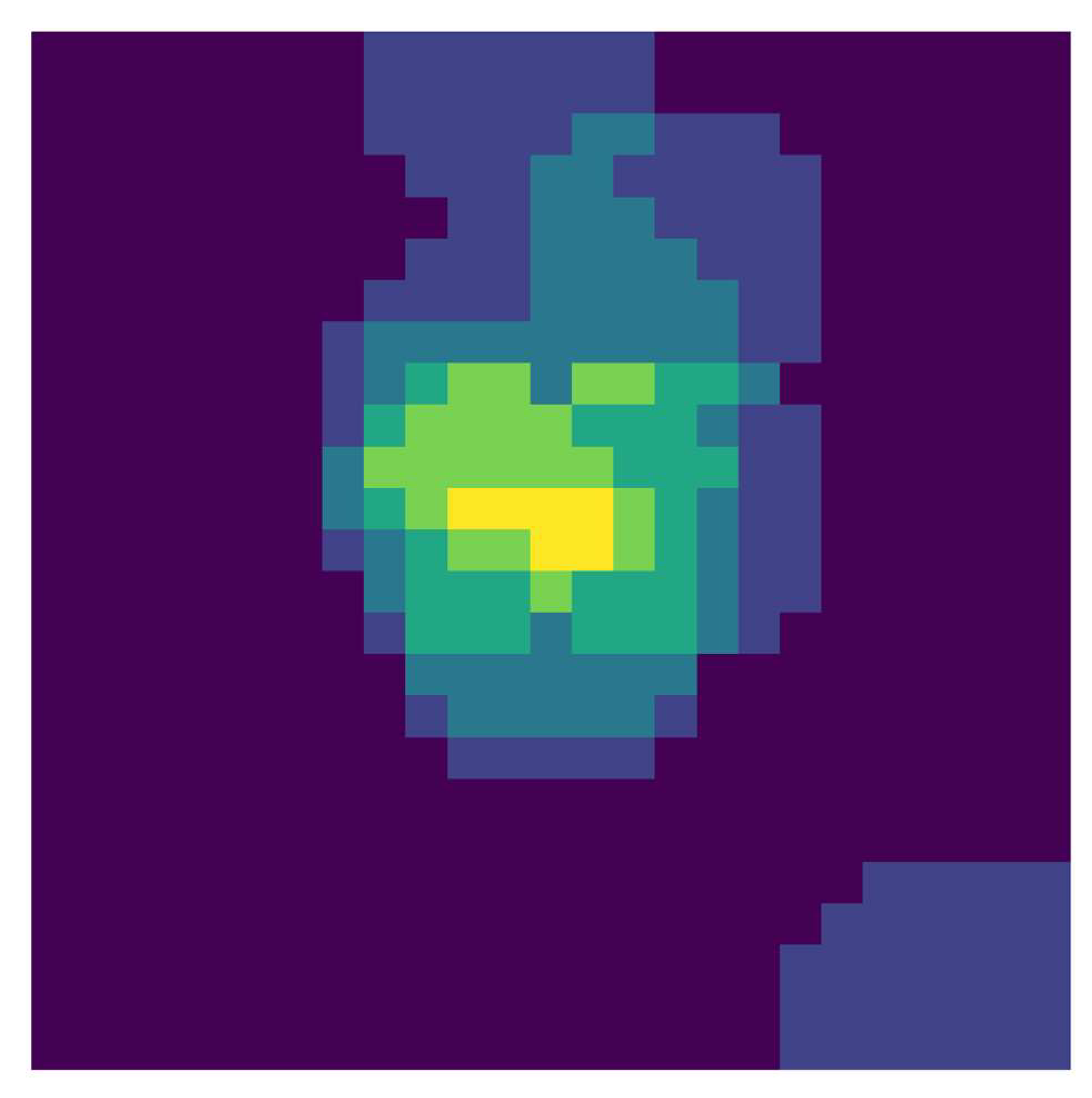
The inputs to the CNN are images with a size of 25 × 25 pixels. A separate image is created for each time step and each variable, and each variable used represents a separate CNN channel. Thus, images of the selected input variables from the previous few hours are fed as input to the CNN. In the center of the image is the target station for which the forecast is generated, and around it are located nearby neighboring stations.

The relative positions of the stations as shown in Figure 1 are determined directly by their geographical coordinates, as given in Table 1. The distance between the target station and the other stations, which is used to determine whether a neighbor station is included in the image, is given by the parameter neighborhood size (ν), described in Section 3.4.3.

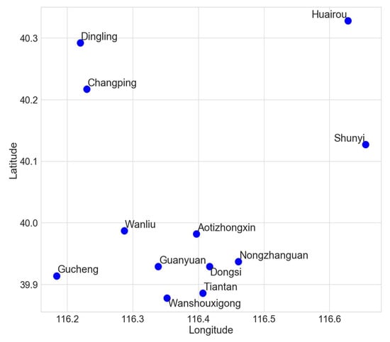
Figure 1. The locations of the 12 stations in the Beijing Multi-Site Air-Quality Data Set.

Table 1. The coordinates of the 12 stations in the Beijing Multi-Site Air-Quality Data Set.

Station	Longitude	Latitude
Aotizhongxin 1	116.397	39.982
Changping	116.23	40.217
Dingling	116.22	40.292
Dongsi	116.417	39.929
Guanyuan	116.339	39.929
Gucheng	116.184	39.914
Huairou	116.628	40.328
Nongzhanguan	116.461	39.937
Shunyi	116.655	40.127
Tiantan	116.407	39.886
Wanliu	116.287	39.987
Wanshouxigong	116.352	39.878

The values of a specific variable at each included neighbor station are represented as circles with a center at the location of the respective station in the image, and a radius r proportional to the value of the variable for the respective station:

$$r=r_{max}\ast x_{var}$$

(9)

$$r_{max}=\raisebox{1ex}{$s_p$}\!\left/ \!\raisebox{-1ex}{$N_{st}$}\right.$$

(10)

where x_var is the normalized value of the corresponding variable, s_p is the number of pixels at one side of the image (in this case the number is 25) and N_st is the number of stations that fall into the neighborhood of the target station (including the target station itself), i.e., the number of stations included in the image.

The value of a specific pixel in the image represents the number of circles of different stations into which it falls inside. Finally, the pixel values are normalized. Thus, the input data are images centered at the target station for which the forecast is generated, and they encode information not only about the value of a certain variable at a certain moment in time, both at the target station and at neighboring stations, but also about the relative spatial positions of the involved stations. Figure 2 shows an example of an input image with a neighborhood size 0.6 for the variable PM_2.5 at 0 h on 29 June 2015, for the target station Dongsi.

Figure 2. An example of an input image with a neighborhood size 0.6 for the variable PM_2.5 at 0 h on 29 June 2015, for the target station Dongsi and its neighbors.

3.4.4. Architecture Optimization

One serious shortcoming in many research studies is the use of a trial and error approach to optimize the proposed models. For this reason, in this study, the network architectures as well as other hyperparameters (as described in Section 3.4.3 and given in Table 2) are optimized by a genetic algorithm with a modified crossover operator for solutions with variable lengths. The evolutionary procedure is implemented as described in [66,67]. The models are trained on the training data for five epochs, and evaluated on the validation data using MAE. The solutions are always evaluated and the fitness score of a certain solution is the average MAE so far.

Table 2. Possible values of the optimized hyperparameters.

	Hyperparameter	Possible Values
Convolutional part	Number of kernels	[16, 32, 64, 128, 256]
	Kernel size	[2, 3, 4, 5, 6, 7, 8, 9]
	Include a max-pooling layer	[True, False]
	Number of LSTM cells	[25, 50, 100, 150, 200, 250]
LSTM part	Include dropout	[True, False]
	Dropout p	[0.1, 0.2, 0.3, 0.4, 0.5]
Global part	Normalized neighborhood size (νnorm)	[0, 0.1, 0.2, 0.3, 0.4, 0.5, 0.6, 0.7, 0.8, 0.9, 1]
	Time lag	[1, 2, 3, 4, 5, 6, 7, 8]

3.4.5. GA Solution Encoding

The GA solution comprises three parts—convolutional, LSTM and global. The convolutional and the LSTM parts of the solution consist of a certain number of layers, each of which is characterized by certain parameters. For convolutional layers, these parameters are the number of kernels, the kernel size and the parameter that defines if the layer should be followed by a max-pooling layer with kernel size 2. For LSTM layers, the parameters are the number of LSTM cells and a parameter that define if a dropout will be used, as well as its p. The global part has two parameters—normalized neighborhood size (ν_norm) and the time lag. The first parameter determines the size of the neighborhood (ν) around the target station for which the forecast is generated, which is calculated as follows:

$$\nu ={\nu }_{norm}\ast 2max\left(dx,dy\right)$$

(11)

$$dx=max\left(x_{center}-x_{min},x_{max}-x_{center}\right)$$

(12)

$$dy=max\left(y_{center}-y_{min},y_{max}-y_{center}\right)$$

(13)

where ν_norm is the normalized neighborhood size with possible values from 0 to 1, with value 0 meaning that only the target station is included in the image, and value 1 meaning that all stations are included; x_center and y_center are the coordinates of the target station; x_min and x_max are the smallest and largest x coordinates from among all 12 stations, respectively; y_min and y_max are the smallest and largest y coordinates from among all 12 stations, respectively. The x coordinate is the value of the longitude and y is the value of the latitude, and no transformations of the latitude and longitude are made due to the small size of the covered area.

The neighborhood is a square centered on the target station, and the image is generated by all stations the coordinates of which fall within this neighborhood. When the size of the neighborhood is small, only the closest stations to the target station are included in the image, while for higher values more distant stations are also included in the image. The second parameter determines the number of historic data samples used by the model; for example, a time lag of 3 means that the data from the previous 3 h will be used as input information.

Table 2 shows the optimized parameters of the network architecture, and the possible values they can have.

3.4.6. Selecting and Training the Best Architecture

The best architectures of the last generation of the evolutionary procedure are selected and then trained on a combination of the training and validation set for 100 epochs, then evaluated on the test set. Due to the stochastic nature of the weight initialization, each training is repeated as 10 independent runs.

3.4.7. Performance Metrics

The following metrics are used to evaluate the performance of the best architectures: mean absolute error (MAE), root mean square error (RMSE) and coefficient of determination (R²).

$$MAE=\frac{{{\displaystyle \sum }}_{i=1}^n\left|y_i-\widehat{y_i}\right|}{n}$$

(14)

$$RMSE=\sqrt{\frac{{{\displaystyle \sum }}_{i=1}^n{\left(y_i-\widehat{y_i}\right)}^2}{n}}$$

(15)

$$R^2=1-\frac{{{\displaystyle \sum }}_{i=1}^n{\left(y_i-\widehat{y_i}\right)}^2}{{{\displaystyle \sum }}_{i=1}^n{\left(y_i-\overline{y}\right)}^2}$$

(16)

where $\widehat{y_i}$ is the predicted value of the i-th sample, $y_i$ is the true value for that sample, n is the total number of samples, and $\overline{y}=\raisebox{1ex}{${{\displaystyle \sum }}^n{y}_i$}\!\left/ \!\raisebox{-1ex}{$n$}\right.$.

4. Experimental Testing and Results

4.1. Experimental Setup

The Keras library is used to implement the models and the Adam algorithm is used in the training, with a learning rate of 0.001, β₁ = 0.9, β₂ = 0.999, ε = 1.0 × 10⁻⁷ and batch size of 16. The training of the network architectures is performed on NVIDIA GeForce RTX 2060. ReLU is used as an activation function not only for the convolutional layers, but also for the LSTM layers. The strides of the convolutional layers are set to (1, 1), and the padding to valid. Max-pooling is used with size (2, 2), strides (2, 2) and valid padding. For the evolutionary optimization, the population size is set to 20, the number of generations to 50, and elitism of size 2 is also used. The maximum number of convolutional layers is set to 10, and the maximum number of LSTM layers to 5.

Due to the limited computational resources, experiments are conducted on 3 of the 12 stations—Dongsi, Wanliu and Changping. All these three stations are selected prior to the experiments so that the target stations are surrounded by other stations. A separate model is optimized for each station, and due to the stochastic nature of the evolutionary search, the optimization of the architecture for each station is repeated three times.

Besides the main experiment for architecture optimization, some additional experiments are also conducted, such as forming various ensembles using the already trained models, validating the proposed hybrid missing data imputation strategy, and validating some components of the proposed spatiotemporal model. In order to make correct comparisons with the results of the main experiment, separate models are optimized for each additional experiment involving the spatiotemporal model, using the already outlined procedure. As in the main experiment, the evolutionary optimization is repeated three times. Due to the limited computational resources, the additional experiments are conducted for only one station—Wanliu (unless explicitly stated otherwise).

4.2. Experimental Results for Architecture Optimization

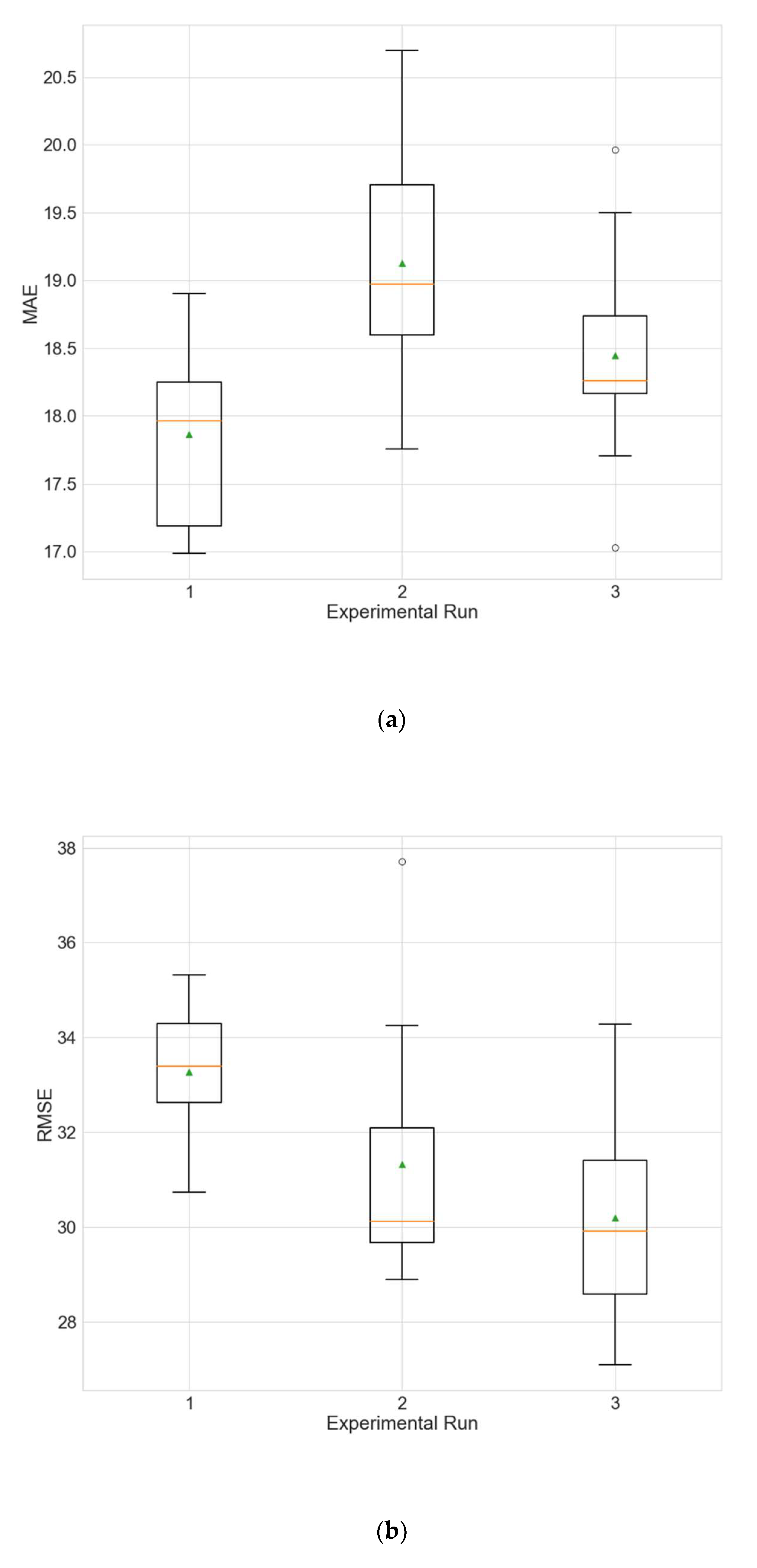
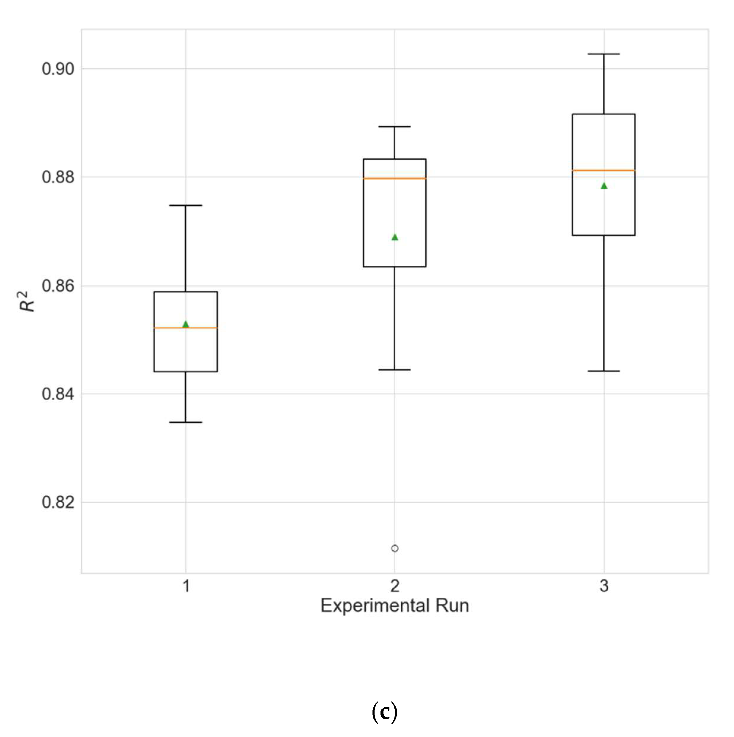
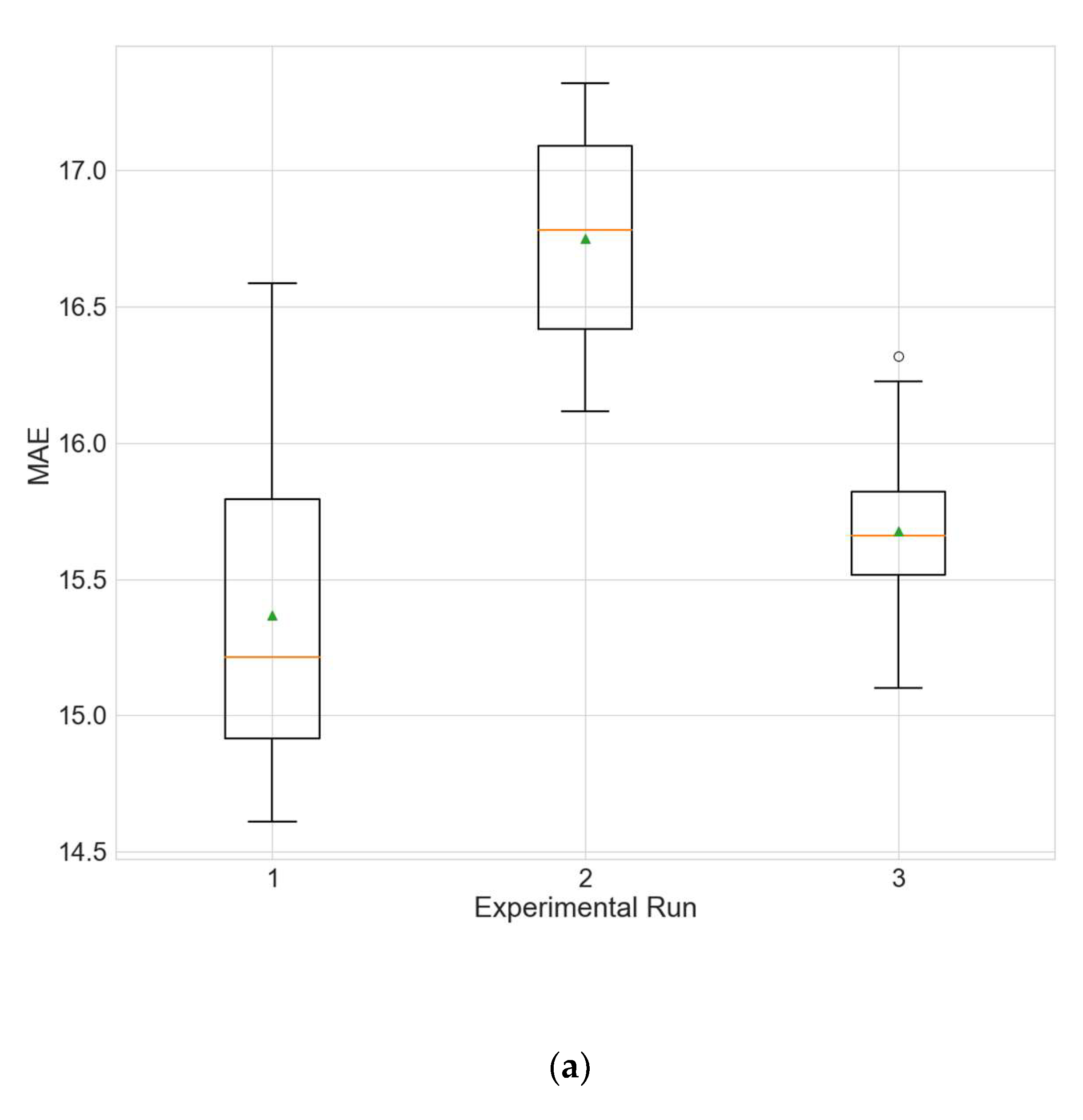
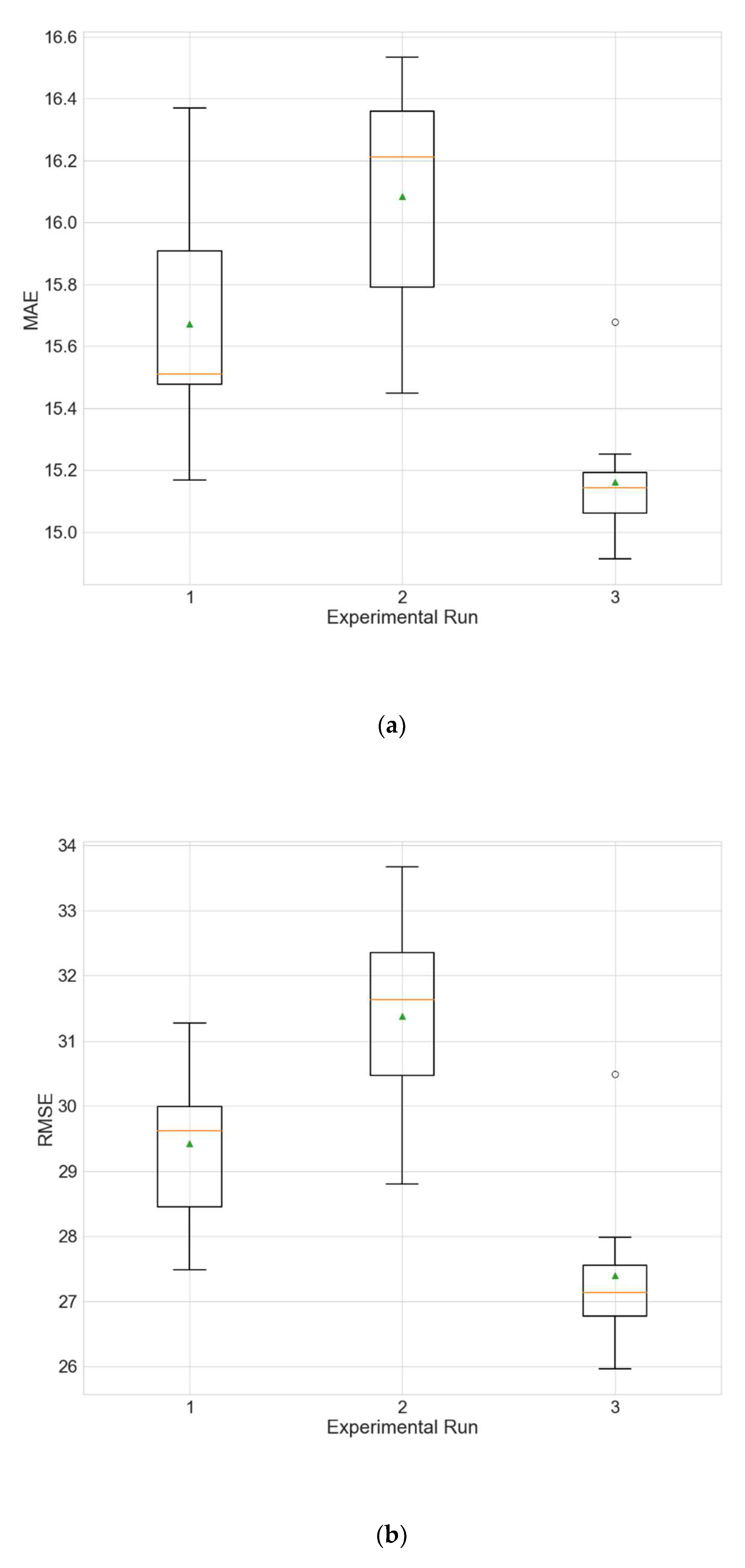
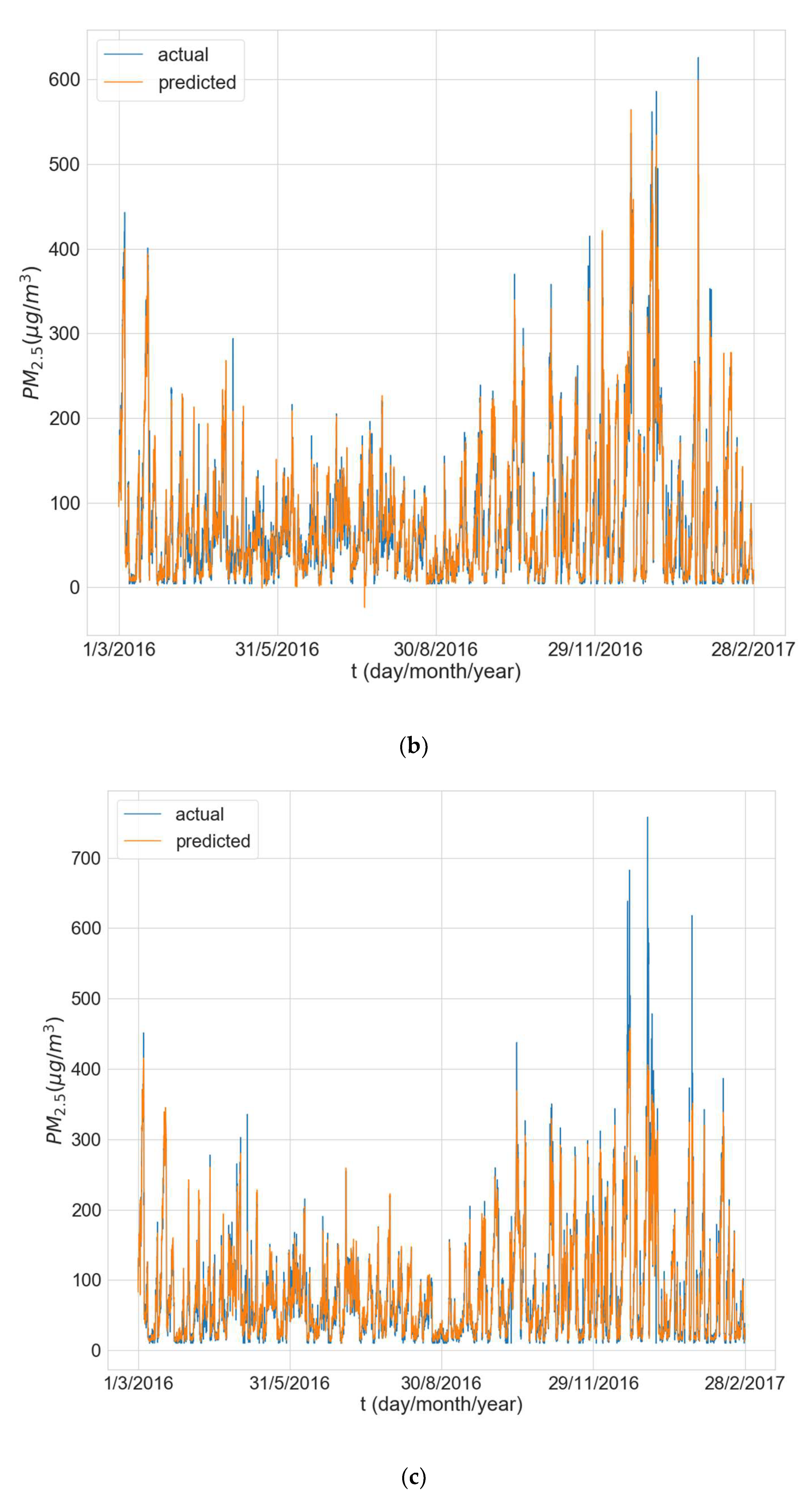
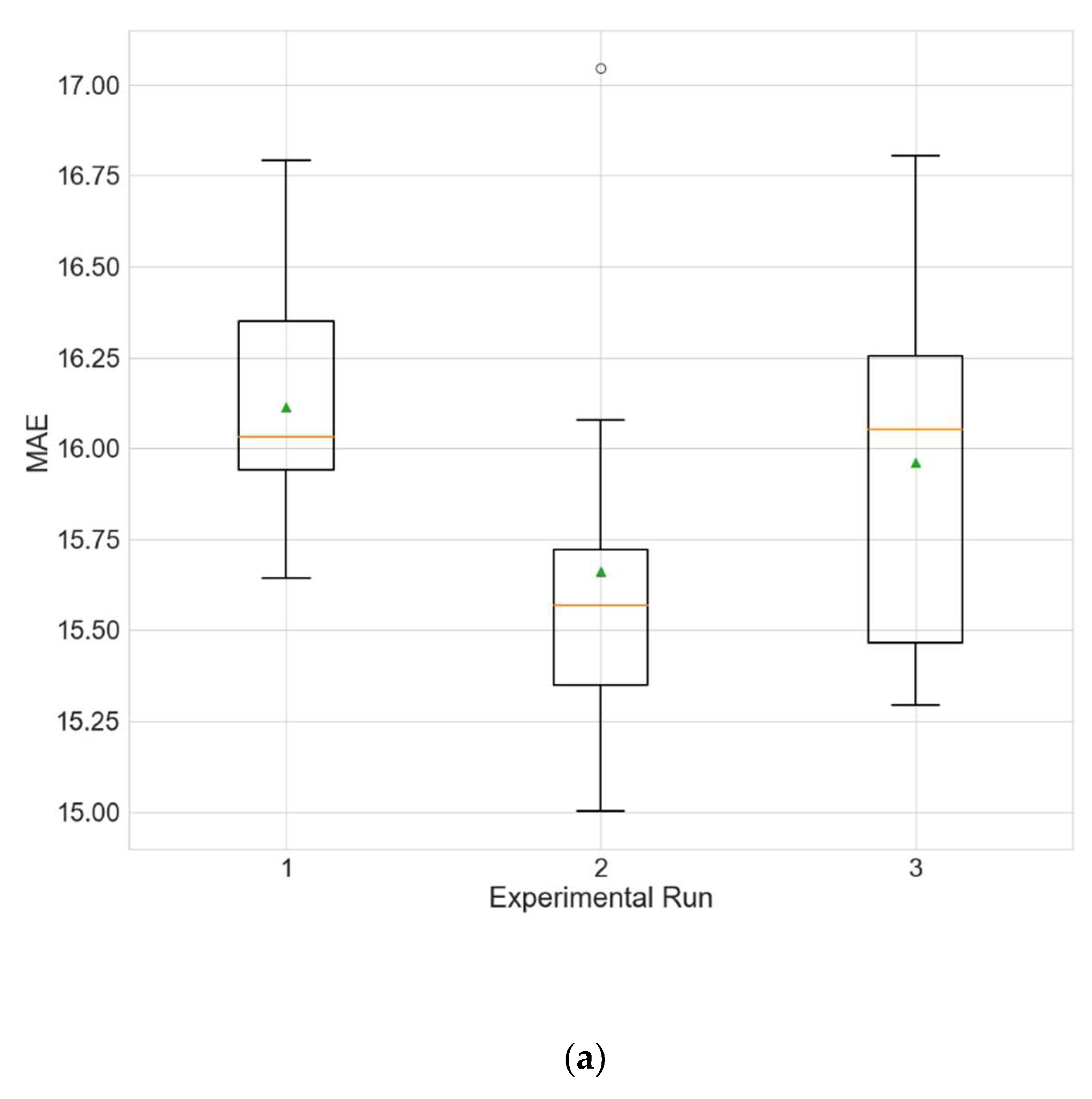
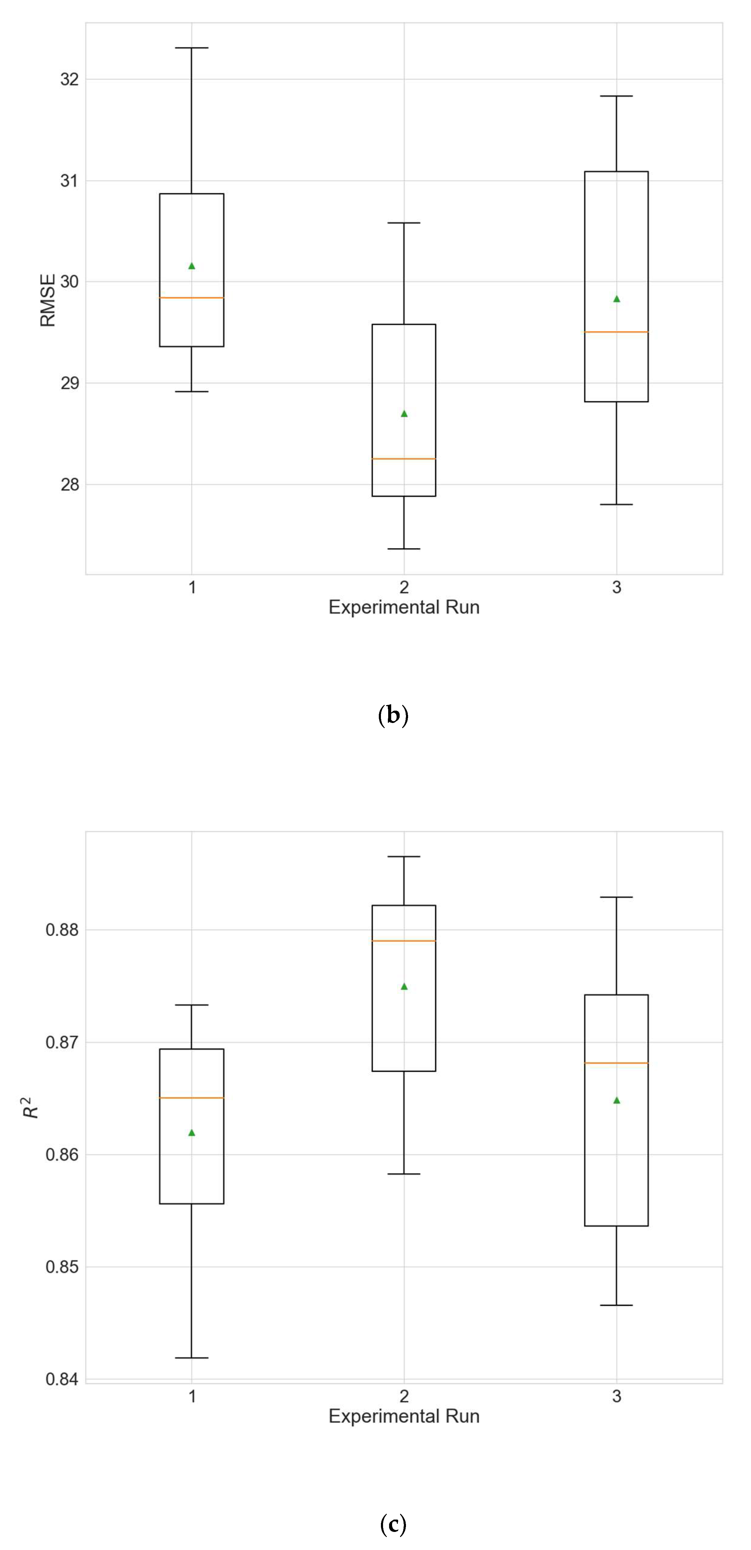
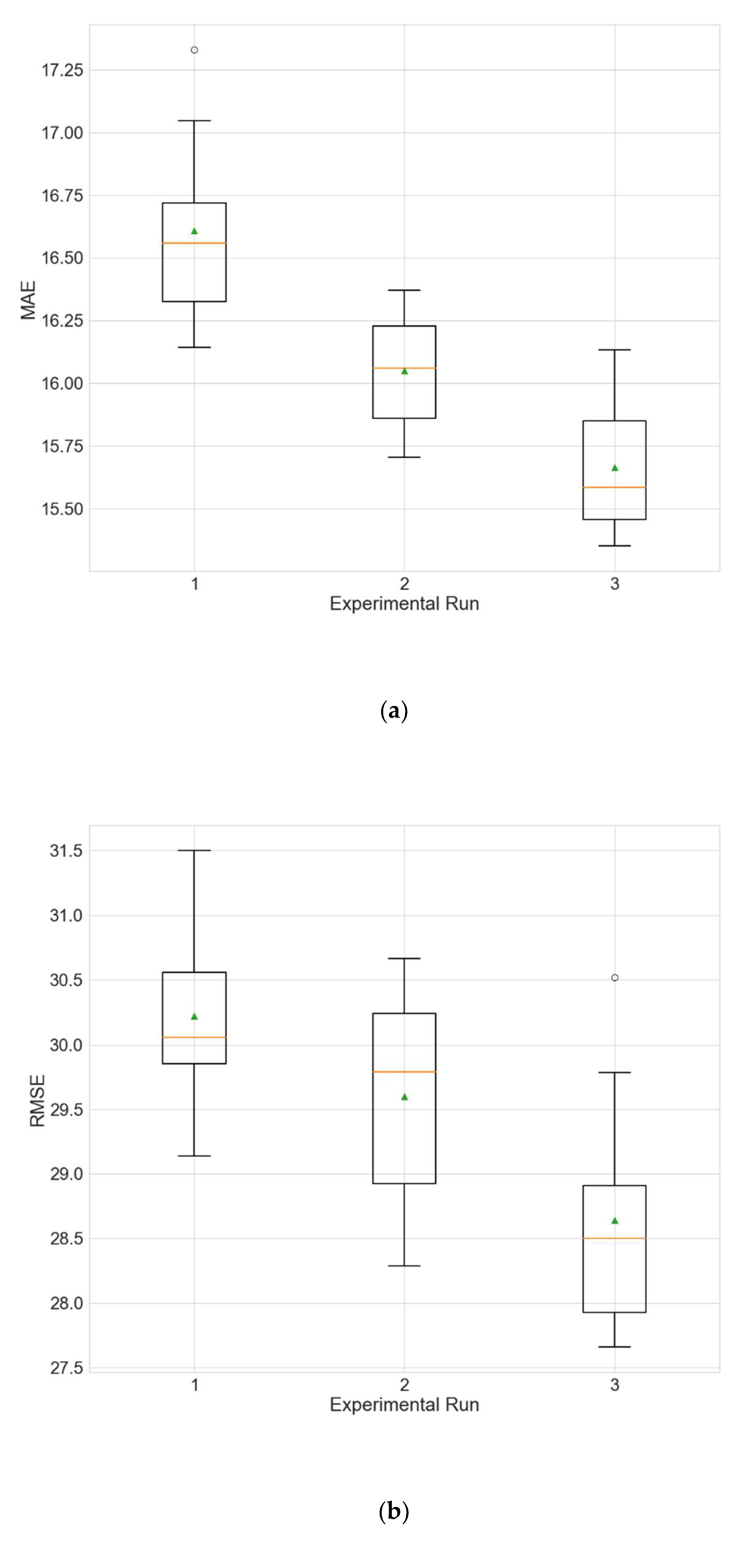
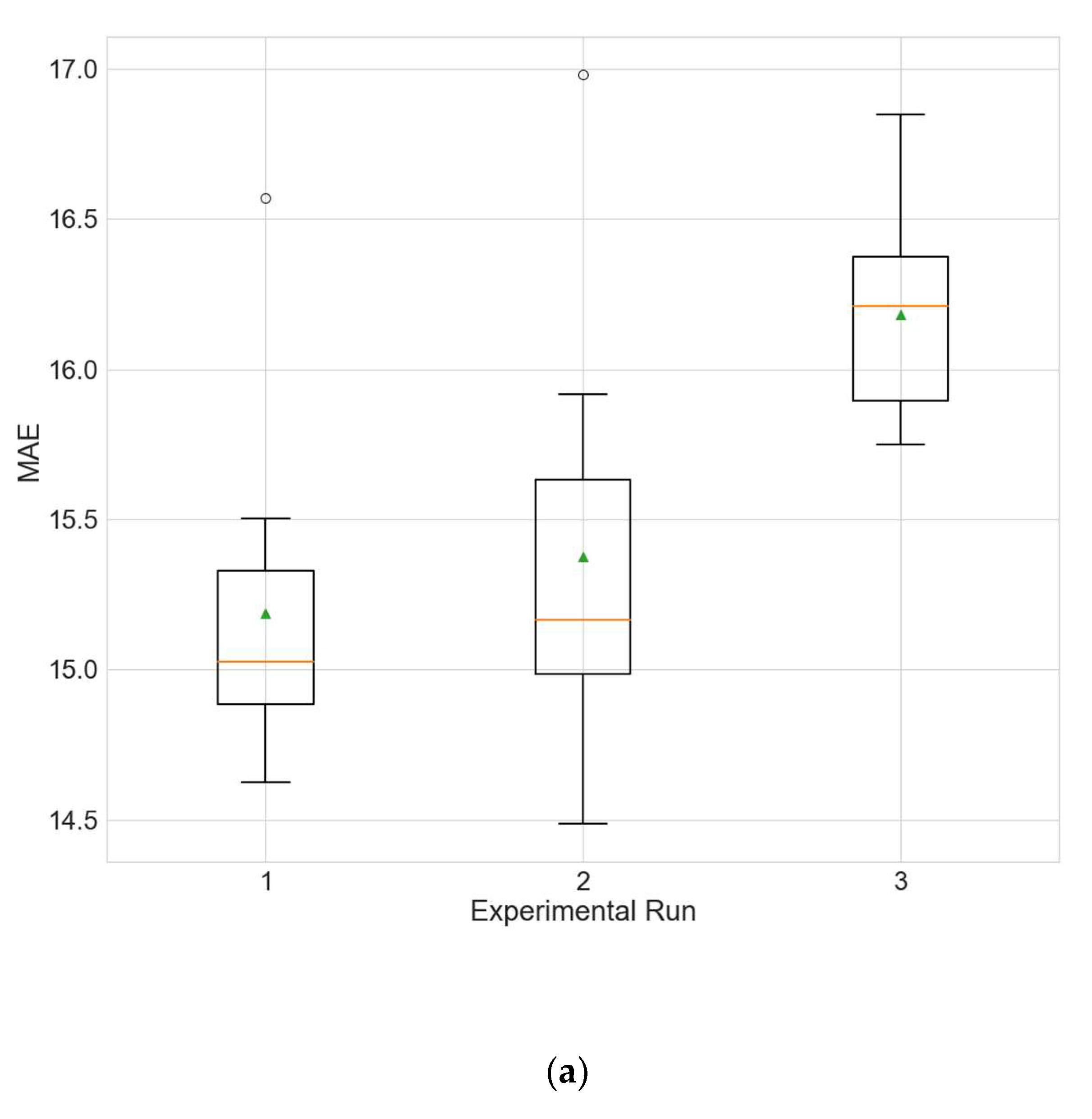
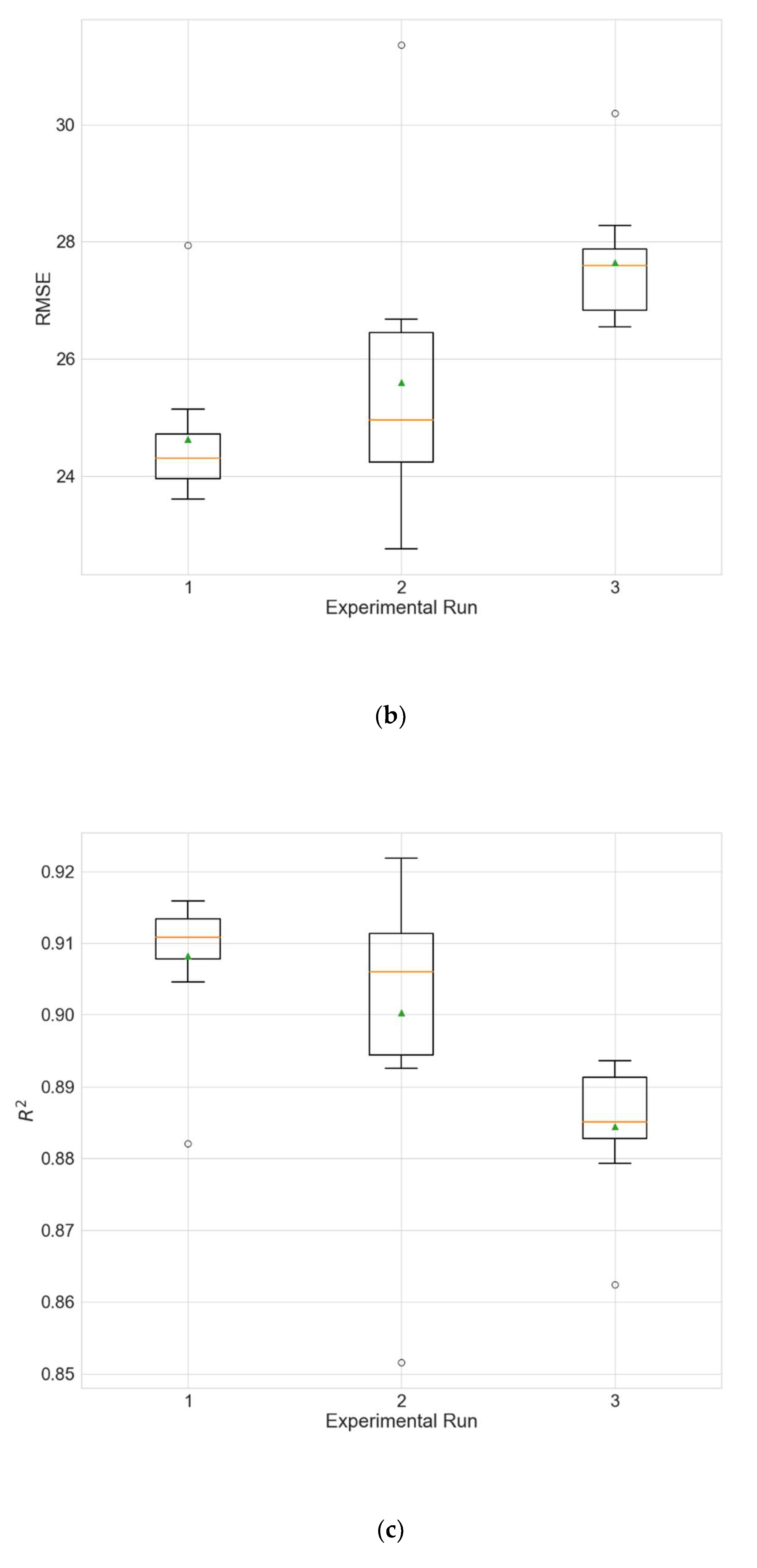
The experimental results for the architecture optimization of the three independent experimental runs for each of the three selected stations are given in Table 3, Table 4 and Table 5. Additionally, the distributions of the performance metrics for each station are depicted as boxplots (including the mean shown as a green triangle) in Figure 3, Figure 4 and Figure 5. The results prove that architectures have been successfully found for each of the stations. Moreover, the models trained using the best architecture provide good and consistent results, with the best performance being achieved for station Wanliu.

Table 3. Performances of the best architecture for station Dongsi for each experimental run. The values are averaged over the 10 independent training runs.

Run	MAE	RMSE	R2
1	17.866 ± 0.672	33.274 ± 1.351	0.853 ± 0.012
2	19.128 ± 0.863	31.326 ± 2.637	0.869 ± 0.023
3	18.446 ± 0.797	30.207 ± 2.076	0.878 ± 0.017

Table 4. Performances of the best architecture for station Wanliu for each experimental run. The values are averaged over the 10 independent training runs.

Run	MAE	RMSE	R2
1	15.370 ± 0.586	25.165 ± 1.652	0.904 ± 0.013
2	16.753 ± 0.384	26.446 ± 0.707	0.894 ± 0.006
3	15.675 ± 0.375	24.714 ± 0.751	0.908 ± 0.006

Table 5. Performances of the best architecture for station Changping for each experimental run. The values are averaged over the 10 independent training runs.

Run	MAE	RMSE	R2
1	15.673 ± 0.374	29.429 ± 1.155	0.869 ± 0.010
2	16.085 ± 0.384	31.382 ± 1.502	0.850 ± 0.014
3	15.161 ± 0.199	27.394 ± 1.165	0.886 ± 0.010

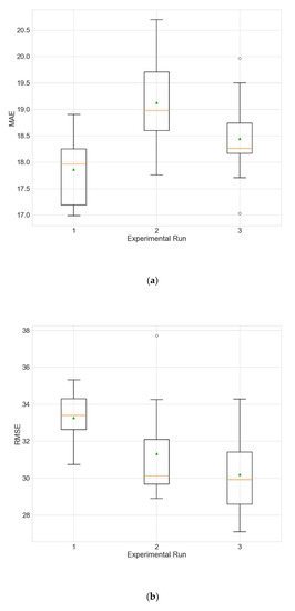
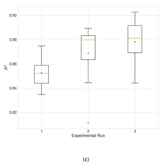
Figure 3. Boxplots showing the distributions of the different performance metrics of the best architecture for station Dongsi. (a) MAE; (b) RMSE; (c) R².

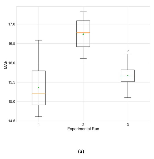
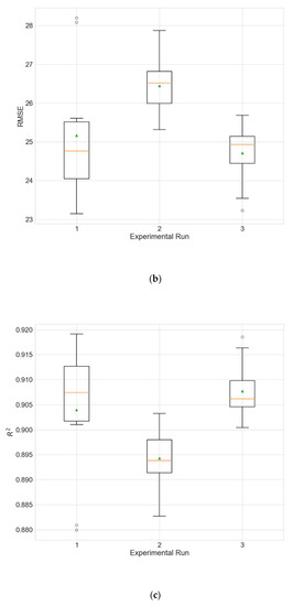
Figure 4. Boxplots showing the distributions of the different performance metrics of the best architecture for station Wanliu. (a) MAE; (b) RMSE; (c) R².

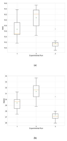
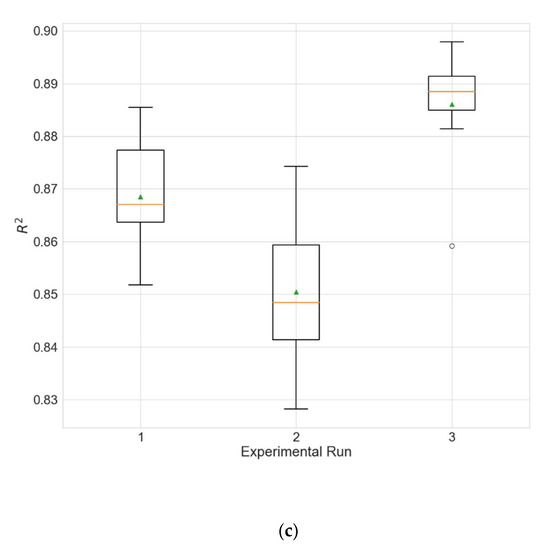
Figure 5. Boxplots showing the distributions of the different performance metrics of the best architecture for station Changping. (a) MAE; (b) RMSE; (c) R².

For comparison of the results achieved by the suggested model, the experimental results for the same three stations from other research studies, using the same data set for PM_2.5 forecasting, are given in Table 6, Table 7 and Table 8. As can be seen, for most of the compared cases, the suggested model does not lag far behind other proposed models according to the MAE, and the results for station Wanliu are comparable to those of some other deep NN models.

Table 6. Comparison of the results of different models using the same data set for forecasting PM_2.5 for station Dongsi.

Model	MAE	RMSE
FBProphet [33]	15.1	20.5
ARIMA [33]	14.1	19.8
LSTM [33]	13.2	21.3
CNN [33]	16.1	22.0
CNN-LSTM [42]	9.653	17.706

Table 7. Comparison of results of different models using the same data set for forecasting PM_2.5 for station Changping.

Model	MAE	RMSE
FBProphet [33]	13.2	18.9
ARIMA [33]	13.3	19.2
LSTM [33]	12.7	18.8
CNN [33]	14.0	20.2
CNN-LSTM [42]	8.873	15.710

Table 8. Comparison of the results of different models using the same data set for forecasting PM_2.5 for station Wanliu.

Model	MAE	RMSE
FBProphet [33]	14.7	19.6
ARIMA [33]	14.2	19.3
LSTM [33]	15.9	23.9
CNN [33]	13.9	23.4
CNN-LSTM [42]	8.486	14.951

The best architectures obtained from each of the three experimental runs for the three selected stations are given in Table 9, Table 10 and Table 11. In most of the cases, a large value of the neighborhood size is used, often 1, i.e., all 12 stations are taken into account, and for Wanliu, in every experimental run, the best architecture uses the maximum size. A large time lag (7 or 8) is also often applied. The results obtained demonstrate the benefits of including spatial information from as many surrounding stations as possible, as well as using as much historical information as possible. Most of the models have one convolutional layer. The convolutional layers most often have a relatively small number of kernels and a small kernel size. In about half of the cases, the convolutional layers are followed by a max-pooling layer. After the convolutional part, one or two LSTM layers are utilized. In about half of the cases, dropout regularization is applied to the LSTM layer using relatively small values of p—0.1, 0.2 and 0.3.

Table 9. The best architecture for each optimization run on station Dongsi. The first row shows the convolutional part, the second the LSTM, and the third the global part. The optimized parameters are given in Table 2.

Run	Architecture
1	[[[64, 5, False]], [[100, True, 0.1], [100, True, 0.2]], [[0.2, 7]]]
2	[[[32, 2, True]], [[100, False, 0.3]], [[1, 7]]]
3	[[[16, 3, True]], [[150, False, 0.5]], [[1, 8]]]

Table 10. The best architecture for each optimization run on station Wanliu. The first row shows the convolutional part, the second the LSTM, and the third the global part. The optimized parameters are given in Table 2.

Run	Architecture
1	[[[64, 2, False], [16, 2, True]], [[150, False, 0.1]], [[1, 6]]]
2	[[[32, 3, True]], [[25, False, 0.2], [250, True, 0.1]], [[1, 5]]]
3	[[[32, 2, False]], [[100, False, 0.2]], [[1, 8]]]

Table 11. The best architecture for each optimization run on station Changping. The first row shows the convolutional part, the second the LSTM, and the third the global part. The optimized parameters are given in Table 2.

Run	Architecture
1	[[[32, 4, True]], [[200, False, 0.1], [150, True, 0.3]], [[0.7, 4]]]
2	[[[16, 6, False]], [[200, True, 0.2], [250, True, 0.3]], [[0.7, 7]]]
3	[[[16, 3, False], [32, 3, True]], [[100, False, 0.5], [25, False, 0.4]], [[0.7, 8]]]

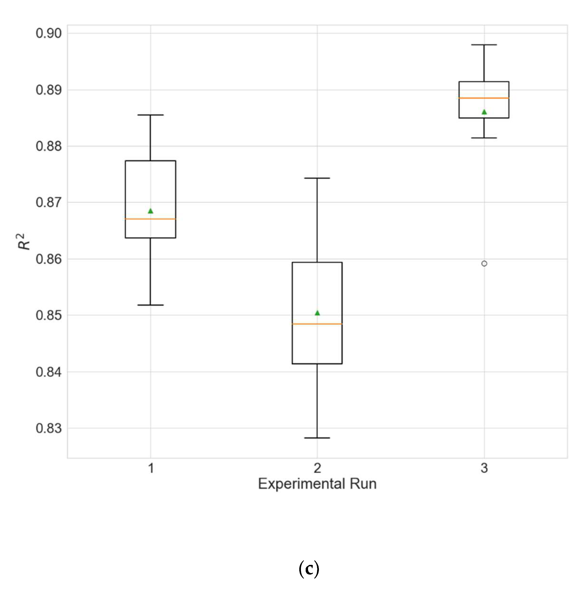
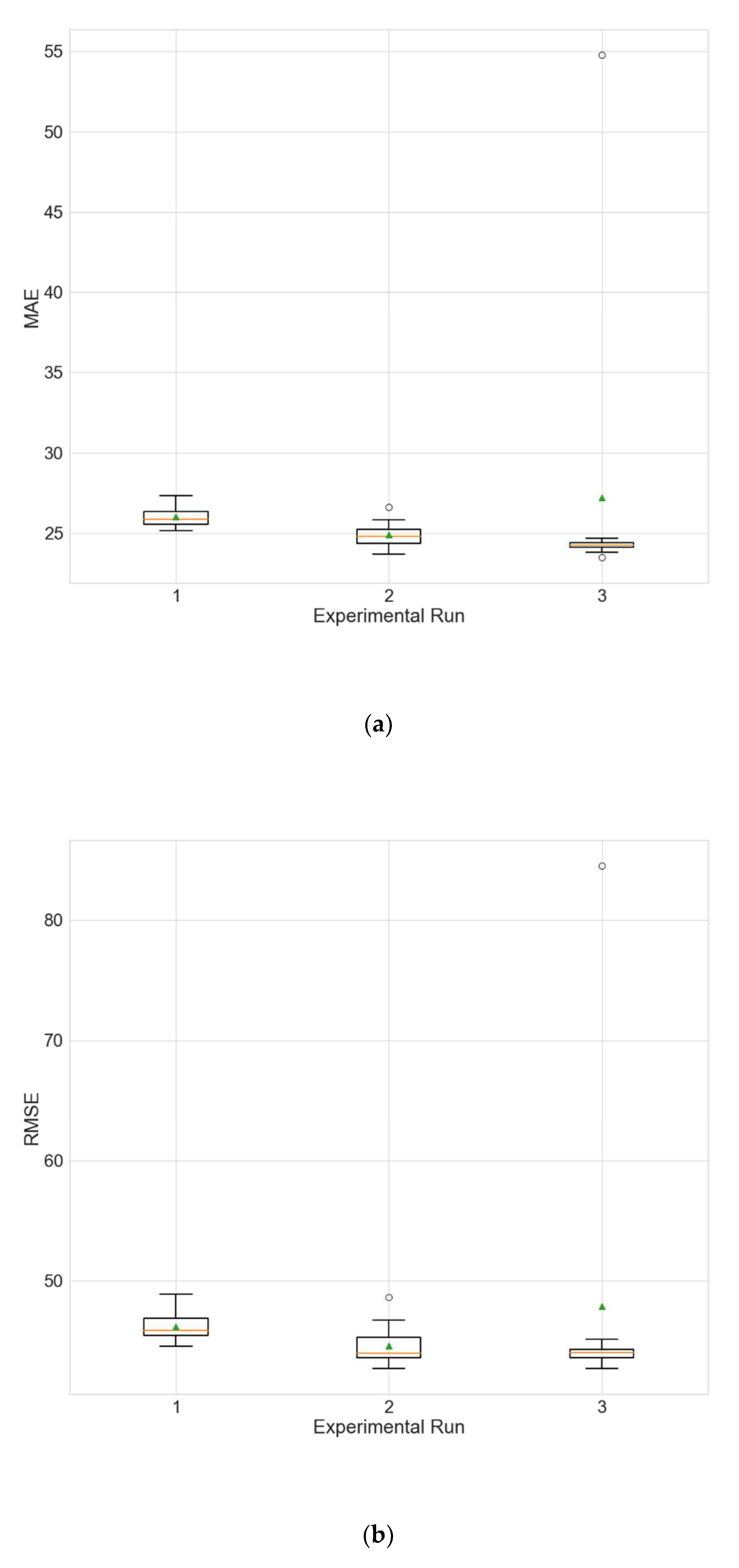
Figure 6 shows the predictions made by the model (averaged over all 10 training runs) over the entire test period vs. the actual values for one of the experimental runs for each of the three stations. The results reveal that the models experience some difficulty in predicting peak concentrations, especially when the peaks are very large, and this is most evident for Changping (Figure 6c).

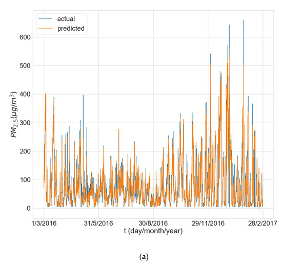
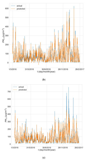
Figure 6. Actual value and average predicted value for the whole test period from the 3rd experimental run for station: (a) Dongsi; (b) Wanliu; (c) Changping.

4.3. Using the Trained Models to Form Ensembles

Additional experiments have been conducted with the formation of ensembles from the already trained models from the main experiment for architecture optimization. Two different strategies for inclusion in the ensembles are tested; the first uses the models from the 10 training runs of the best architecture obtained from a single optimization run (i.e., an ensemble of models with the same architecture), and the other uses the k best models from the training runs from each experimental run (i.e., an ensemble including models with different architectures). In all cases, the final forecast is obtained by averaging the individual forecasts of the models in the ensemble.

Table 12, Table 13 and Table 14 show the results of the ensembles of models with the same architecture and Table 15, Table 16 and Table 17 show the results of the ensemble models with different architectures. As can be seen in all cases, the results improve when using an ensemble of models compared to the individual models from the main experiment (Table 3, Table 4 and Table 5).

Table 12. Results for station Dongsi of the ensemble composed only of models obtained from the 10 independent training runs of the best architecture of a single optimization run.

Run	MAE	RMSE	R2
1	15.636	29.538	0.884
2	16.652	27.136	0.902
3	15.832	26.018	0.910

Table 13. Results for station Wanliu of the ensemble composed only of models obtained from the 10 independent training runs of the best architecture of a single optimization run.

Run	MAE	RMSE	R2
1	13.350	21.359	0.931
2	13.835	21.843	0.928
3	13.746	21.623	0.929

Table 14. Results for station Changping of the ensemble composed only of models obtained from the 10 independent training runs of the best architecture of a single optimization run.

Run	MAE	RMSE	R2
1	13.888	26.805	0.891
2	14.432	28.850	0.874
3	13.126	24.649	0.908

Table 15. Results for station Dongsi of the ensembles of k best models from each optimization run.

Run	MAE	RMSE	R2
1	15.118	25.404	0.9144
2	14.875	25.065	0.9167
3	14.837	24.912	0.9177
4	14.858	25.079	0.9166
5	14.857	25.236	0.9156
6	14.939	25.386	0.9146
7	14.871	25.232	0.9156
8	14.863	25.205	0.9158
9	14.910	25.421	0.9143
10	14.985	25.621	0.9130

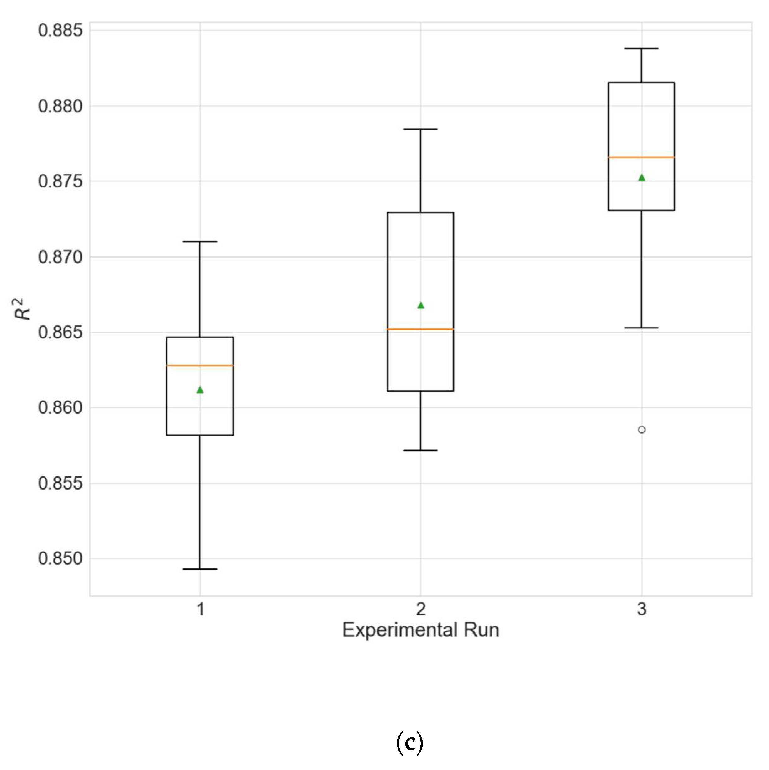
Table 16. Results for station Wanliu of the ensembles of k best models from each optimization run.

Run	MAE	RMSE	R2
1	13.876	21.529	0.9300
2	13.498	21.034	0.9332
3	13.355	20.945	0.9338
4	13.265	20.841	0.9344
5	13.226	20.783	0.9348
6	13.185	20.786	0.9348
7	13.177	20.763	0.9349
8	13.167	20.739	0.9351
9	13.175	20.741	0.9351
10	13.217	20.836	0.9345

Table 17. Results for station Changping of the ensembles of k best models from each optimization run.

Run	MAE	RMSE	R2
1	13.859	25.052	0.9049
2	13.454	24.928	0.9059
3	13.391	25.000	0.9053
4	13.384	25.140	0.9043
5	13.351	25.308	0.9030
6	13.375	25.473	0.9017
7	13.401	25.665	0.9002
8	13.436	25.839	0.8988
9	13.475	26.031	0.8973
10	13.514	26.275	0.8954

With the exception of station Changping, in most cases, an ensemble of k best models from each experimental run gives better results than the strategy of using only models with the same architecture, and the observation is valid for most of the values of k. The comparison between the results of the ensembles with the k best models and the average results (over the three experimental runs) of the ensembles with the same architectures proves that the strategy with the k best models provides better results for all stations.

The overall evaluation of the results indicates that the strategy with the k best models shows better results; for station Dongsi, the best results using that strategy are achieved using k = 3, while for Wanliu they are obtained using k = 8, and for Changping using k = 2. A possible explanation for the higher value of k for Wanliu could be that in the main experiment of architecture optimization, the results for this station are the most consistent, which allows the inclusion of a larger number of models in the ensemble without deteriorating its overall performance.

Comparing the results with those of other research studies using the same data set and predicting PM_2.5 (Table 6, Table 7 and Table 8) demonstrates that for stations Dongsi and Changping, the ensembles have MAE values comparable to most models from [33], but fall behind according to the RMSE, which means that the models probably make big errors more often. However, on the other hand, it should be noted that the forecasts reported in [33] are made on a daily basis, while in the current study, the data in the used dataset are gathered hourly, which may offer an explanation for the lower RMSE. For Wanliu, the ensembles surpass the results achieved in [33] when MAE is used as a metric, and for RMSE the results surpass two of the models—CNN and LSTM, and are slightly behind the other two.

4.4. Validation of the Hybrid Strategy for Missing Data Imputation

Two types of experiments have been performed to validate the proposed strategy for missing data imputation. For the first type, random artificial gaps are generated in the data of each variable (except for the wind direction, which is not included in this experiment), i.e., valid values are removed from randomly selected time intervals. In this way, an additional ~5% of the valid values have been removed for each time series. The gaps sizes are generated using a geometric distribution with p = 0.05. Three strategies are used to fill in the missing values—linear interpolation (LI), the average between the previous value and the average value for the same hour of the same day and month for other years (MTP), and a hybrid approach (HS) that is a combination of the first two. The performance of the strategies is evaluated by R² only on the simulated gaps, i.e., the original missing values are not taken into account in the evaluation.

Due to the stochastic nature of the gap generation, each strategy is evaluated for each variable by 100 independent runs with different simulated gaps. The Kruskal–Wallis (KW) test is used to check for differences between the strategies. The performances of the three strategies applied to data from the three selected stations (Dongsi, Wanliu and Changping) are presented in Table 18, Table 19 and Table 20. The presented values of p in the tables have not been corrected for multiple comparisons.

Table 18. Results of the three missing data imputation strategies for station Dongsi. $\overline{R^2}$ is the average $R^2$ of the 100 independent evaluations.

Variable	LI $\overline{{\mathit{R}}^2}\pm \mathit{\sigma }$	MTP $\overline{{\mathit{R}}^2}\pm \mathit{\sigma }$	HS $\overline{{\mathit{R}}^2}\pm \mathit{\sigma }$	LI vs. MTP		LI vs. HS		MTP vs. HS
				H	p	H	p	H	p
PM2.5	0.9758 ± 0.0084	0.9399 ± 0.0132	0.9737 ± 0.0085	143.99	3.58 × 10−33	4.79	0.0286	144.05	3.47 × 10−33
PM10	0.9724 ± 0.0089	0.9404 ± 0.0155	0.9715 ± 0.0087	135.44	2.65 × 10−31	1.29	0.2559	135.10	3.14 × 10−31
SO2	0.9762 ± 0.0091	0.9500 ± 0.0103	0.9746 ± 0.0092	130.59	3.04 × 10−30	2.24	0.1342	127.21	1.67 × 10−29
NO2	0.9622 ± 0.0070	0.9435 ± 0.0073	0.9629 ± 0.0068	127.65	1.34 × 10−29	0.31	0.5758	132.84	9.82 × 10−31
CO	0.9726 ± 0.0104	0.9412 ± 0.0152	0.9694 ± 0.0110	127.32	1.58 × 10−29	5.35	0.0207	115.79	5.28 × 10−27
O3	0.9600 ± 0.0264	0.9732 ± 0.0153	0.9668 ± 0.0131	82.13	1.27 × 10−19	16.73	4.31 × 10−05	54.20	1.81 × 10−13
TEMP	0.9929 ± 0.0008	0.9944 ± 0.0007	0.9932 ± 0.0009	112.76	2.43 × 10−26	8.54	0.0035	79.62	4.53 × 10−19
PRES	0.9958 ± 0.0018	0.9824 ± 0.0033	0.9950 ± 0.0021	148.90	3.02 × 10−34	9.21	0.0024	148.84	3.11 × 10−34
DEWP	0.9965 ± 0.0011	0.9879 ± 0.0022	0.9959 ± 0.0012	149.25	2.52 × 10−34	14.85	0.0001	149.25	2.52 × 10−34
RAIN	0.9200 ± 0.1036	0.9434 ± 0.0464	0.9229 ± 0.1024	0.35	0.5560	0.05	0.8259	0.77	0.3791
WSPM	0.9491 ± 0.0083	0.9479 ± 0.0076	0.9495 ± 0.0080	0.92	0.3369	0.24	0.6233	2.21	0.1374

Table 19. Results of the three missing data imputation strategies for station Wanliu. $\overline{R^2}$ is the average $R^2$ of the 100 independent evaluations.

Variable	LI $\overline{{\mathit{R}}^2}\pm \mathit{\sigma }$	MTP $\overline{{\mathit{R}}^2}\pm \mathit{\sigma }$	HS $\overline{{\mathit{R}}^2}\pm \mathit{\sigma }$	LI vs. MTP		LI vs. HS		MTP vs. HS
				H	p	H	p	H	p
PM2.5	0.9764 ± 0.0089	0.9376 ± 0.0120	0.9755 ± 0.0090	145.69	1.52 × 10−33	0.46	0.4954	144.05	3.47 × 10−33
PM10	0.9713 ± 0.0088	0.9410 ± 0.0100	0.9686 ± 0.0088	140.37	2.20 × 10−32	6.68	0.0097	135.95	2.04 × 10−31
SO2	0.9785 ± 0.0090	0.9446 ± 0.0142	0.9742 ± 0.0122	137.09	1.15 × 10−31	7.58	0.0059	117.32	2.44 × 10−27
NO2	0.9693 ± 0.0048	0.9447 ± 0.0084	0.9670 ± 0.0067	147.29	6.78 × 10−34	4.76	0.0291	137.72	8.37 × 10−32
CO	0.9774 ± 0.0075	0.9528 ± 0.0126	0.9721 ± 0.0097	127.43	1.50 × 10−29	14.77	0.0001	90.62	1.74 × 10−21
O3	0.9576 ± 0.0086	0.9716 ± 0.0052	0.9607 ± 0.0072	108.29	2.32 × 10−25	6.04	0.0140	91.74	9.89 × 10−22
TEMP	0.9909 ± 0.0011	0.9942 ± 0.0007	0.9917 ± 0.0010	146.99	7.87 × 10−34	24.72	6.62 × 10−07	138.07	7.04 × 10−32
PRES	0.9962 ± 0.0014	0.9829 ± 0.0028	0.9947 ± 0.0021	149.25	2.52 × 10−34	28.40	9.87 × 10−08	148.90	3.02 × 10−34
DEWP	0.9969 ± 0.0009	0.9895 ± 0.0017	0.9962 ± 0.0012	149.19	2.60 × 10−34	16.27	5.48 × 10−05	149.07	2.76 × 10−34
RAIN	0.9269 ± 0.1467	0.9442 ± 0.0538	0.9422 ± 0.0692	1.61	0.2039	0.13	0.7158	0.59	0.4429
WSPM	0.9443 ± 0.0088	0.9513 ± 0.0072	0.9475 ± 0.0078	30.84	2.79 × 10−08	6.90	0.0086	10.66	0.0011

Table 20. Results of the three missing data imputation strategies for station Changping. $\overline{R^2}$ is the average $R^2$ of the 100 independent evaluations.

Variable	LI $\overline{{\mathit{R}}^2}\pm \mathit{\sigma }$	MTP $\overline{{\mathit{R}}^2}\pm \mathit{\sigma }$	HS $\overline{{\mathit{R}}^2}\pm \mathit{\sigma }$	LI vs. MTP		LI vs. HS		MTP vs. HS
				H	p	H	p	H	p
PM2.5	0.9766 ± 0.0093	0.9389 ± 0.0104	0.9737 ± 0.0094	141.07	1.55 × 10−32	5.61	0.0179	143.64	4.27 × 10−33
PM10	0.9706 ± 0.0111	0.9439 ± 0.0109	0.9700 ± 0.0103	123.16	1.28 × 10−28	0.66	0.4158	123.98	8.52 × 10−29
SO2	0.9772 ± 0.0097	0.9489 ± 0.0141	0.9744 ± 0.0104	122.62	1.69 × 10−28	5.44	0.0196	113.13	2.02 × 10−26
NO2	0.9676 ± 0.0061	0.9479 ± 0.0082	0.9661 ± 0.0060	134.70	3.84 × 10−31	3.04	0.0815	129.31	5.80 × 10−30
CO	0.9754 ± 0.0093	0.9474 ± 0.0138	0.9755 ± 0.0086	129.37	5.64 × 10−30	2.39 × 10−05	0.9961	131.82	1.63 × 10−30
O3	0.9616 ± 0.0078	0.9721 ± 0.0054	0.9657 ± 0.0069	80.98	2.28 × 10−19	12.50	0.0004	41.26	1.33 × 10−10
TEMP	0.9923 ± 0.0009	0.9939 ± 0.0010	0.9928 ± 0.0008	86.30	1.55 × 10−20	15.17	9.83 × 10−05	59.01	1.57 × 10−14
PRES	0.9963 ± 0.0012	0.9832 ± 0.0028	0.9952 ± 0.0018	149.25	2.52 × 10−34	25.11	5.40 × 10−07	149.13	2.68 × 10−34
DEWP	0.9971 ± 0.0010	0.9885 ± 0.0017	0.9964 ± 0.0011	149.19	2.60 × 10−34	22.77	1.82 × 10−06	149.25	2.52 × 10−34
RAIN	0.9309 ± 0.0950	0.9342 ± 0.0554	0.9288 ± 0.0891	1.25	0.2642	0.04	0.8355	0.78	0.3764
WSPM	0.9485 ± 0.0077	0.9492 ± 0.0080	0.9505 ± 0.0086	0.25	0.6182	3.42	0.0644	1.61	0.2048

As seen from the results, taking into account the multiple comparisons (11 variables per station), in most cases there is no significant difference between the linear interpolation and the hybrid strategy for the pollutant data (except for ozone, where the hybrid strategy shows better results for two of the stations).

The MTP strategy gives the weakest results for all pollutants except ozone, where it outperforms both linear interpolation and the hybrid strategy. Regarding the meteorological variables, there is no significant difference in the performances of the three strategies for precipitation and wind speed in almost all cases. The MTP strategy performs best compared to the other two for the temperature, and shows the weakest results for pressure and dew point temperature. Compared to the other two strategies, linear interpolation performs worst for temperature, but shows the best results for pressure and dew point temperature. For these variables, the hybrid strategy gives results between those of the other two strategies. Out of all variables, linear interpolation and the hybrid strategy show the weakest results for precipitation and wind speed, which may be due to the complex and chaotic nature of these two phenomena. The results reveal that the hybrid strategy is not inferior to the linear interpolation strategy in most cases, and even surpasses it for some specific variables, such as ozone and temperature. For these variables, the seasonal patterns are characterized by less noise than other variables in the selected data set, and the hybrid strategy manages to account better for the seasonal dependencies.

In the second type of experiments, the missing value imputation strategies are evaluated by the performance of models trained with the filled data. Two additional experiments are performed; the first one utilizes models optimized using data imputation by linear interpolation, and the second one utilizes models using data imputation with the MTP strategy. These two experiments are performed using the data from station Changping due to the presence of a larger number of large gaps compared to the data at station Wanliu, which makes Changping a better choice for the testing of the different imputation strategies.

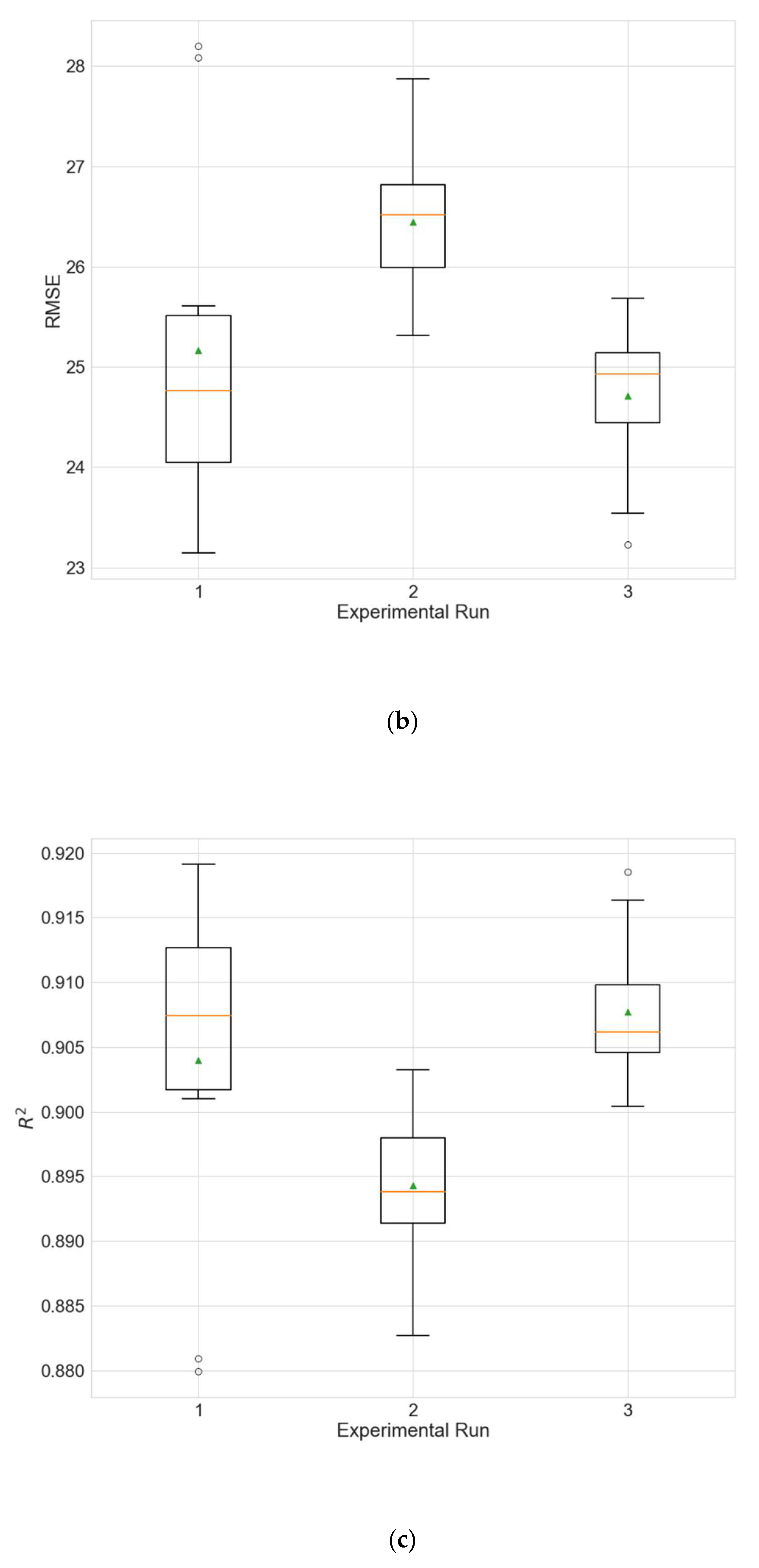
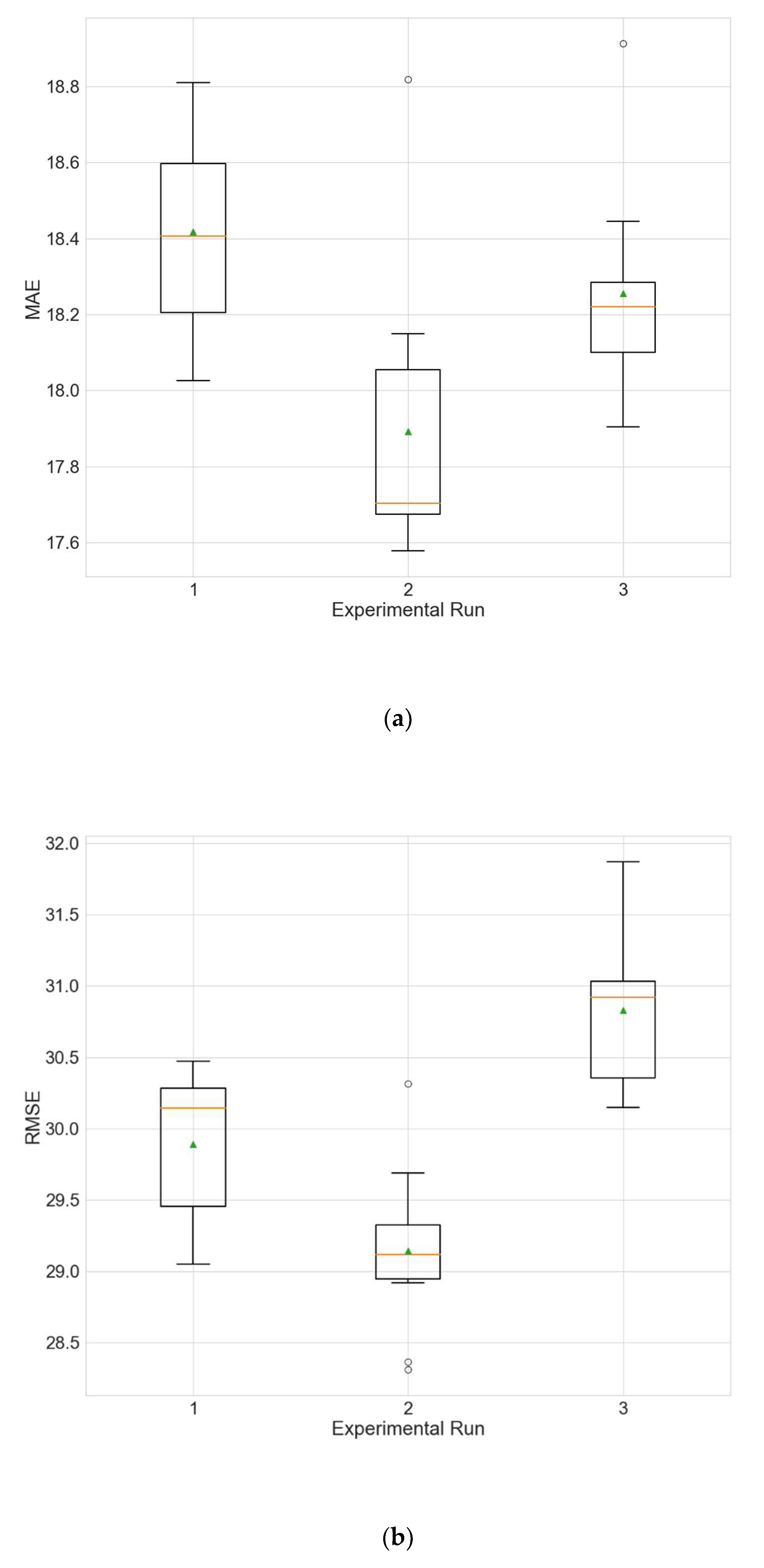
Table 21 and Table 22 show the results of the two above described experiments. Figure 7 and Figure 8 depict the distributions of the different performance metrics as a boxplot. The results obtained for the training runs from all experimental runs are compared with those for the main experiment that uses the hybrid strategy (Table 5) via a KW test. No significant differences can be observed between the hybrid strategy and the linear interpolation (for all metrics p is above 0.05). A possible explanation for this observation, given the results of the first type of experiments (Table 18, Table 19 and Table 20), is that the variables for which the hybrid strategy has an advantage over linear interpolation (ozone and temperature) are not selected by the initial random search as input variables. The hybrid strategy produces better MAE compared to the MTP strategy (p = 0.0014).

Table 21. Performance of the best architecture for station Changping for each experimental run, using data filled only by linear interpolation. The values are averaged over the 10 independent training runs.

Run	MAE	RMSE	R2
1	16.115 ± 0.336	30.159 ± 1.035	0.862 ± 0.010
2	15.662 ± 0.544	28.700 ± 1.017	0.875 ± 0.009
3	15.961 ± 0.488	29.836 ± 1.332	0.865 ± 0.012

Table 22. Performance of the best architecture for station Changping for each experimental run, using data filled with the MTP strategy. The values are averaged over the 10 independent training runs.

Run	MAE	RMSE	R2
1	16.608 ± 0.348	30.219 ± 0.722	0.861 ± 0.007
2	16.051 ± 0.223	29.598 ± 0.769	0.867 ± 0.007
3	15.664 ± 0.255	28.644 ± 0.865	0.875 ± 0.008

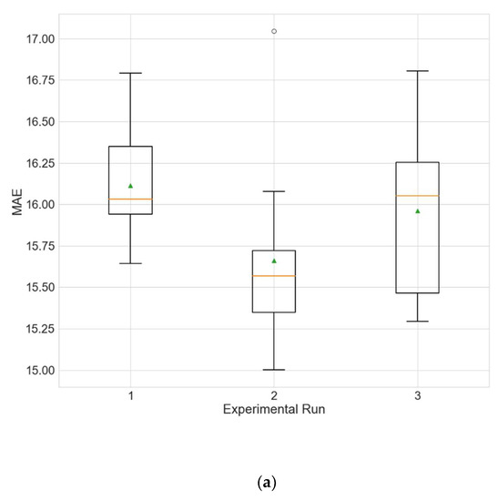
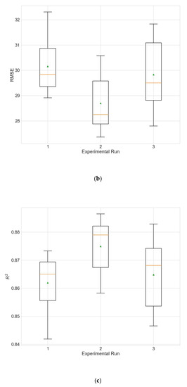
Figure 7. Boxplot showing the distributions of the different performance metrics of the best architecture for station Changping from the experiment that uses data filled only by linear interpolation. (a) MAE; (b) RMSE; (c) R².

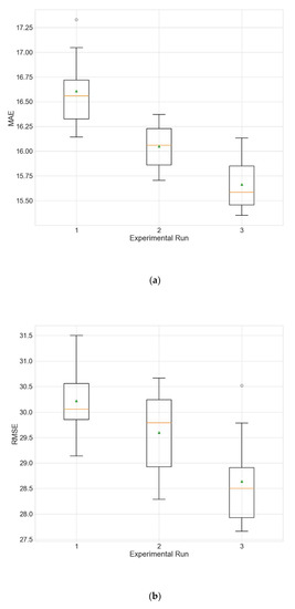
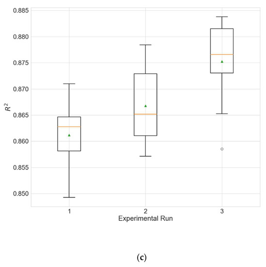
Figure 8. Boxplot showing the distributions of the different performance metrics of the best architecture for station Changping from the experiment that uses data filled with the MTP strategy. (a) MAE; (b) RMSE; (c) R².

4.5. Selection of Input Variables by Random Search

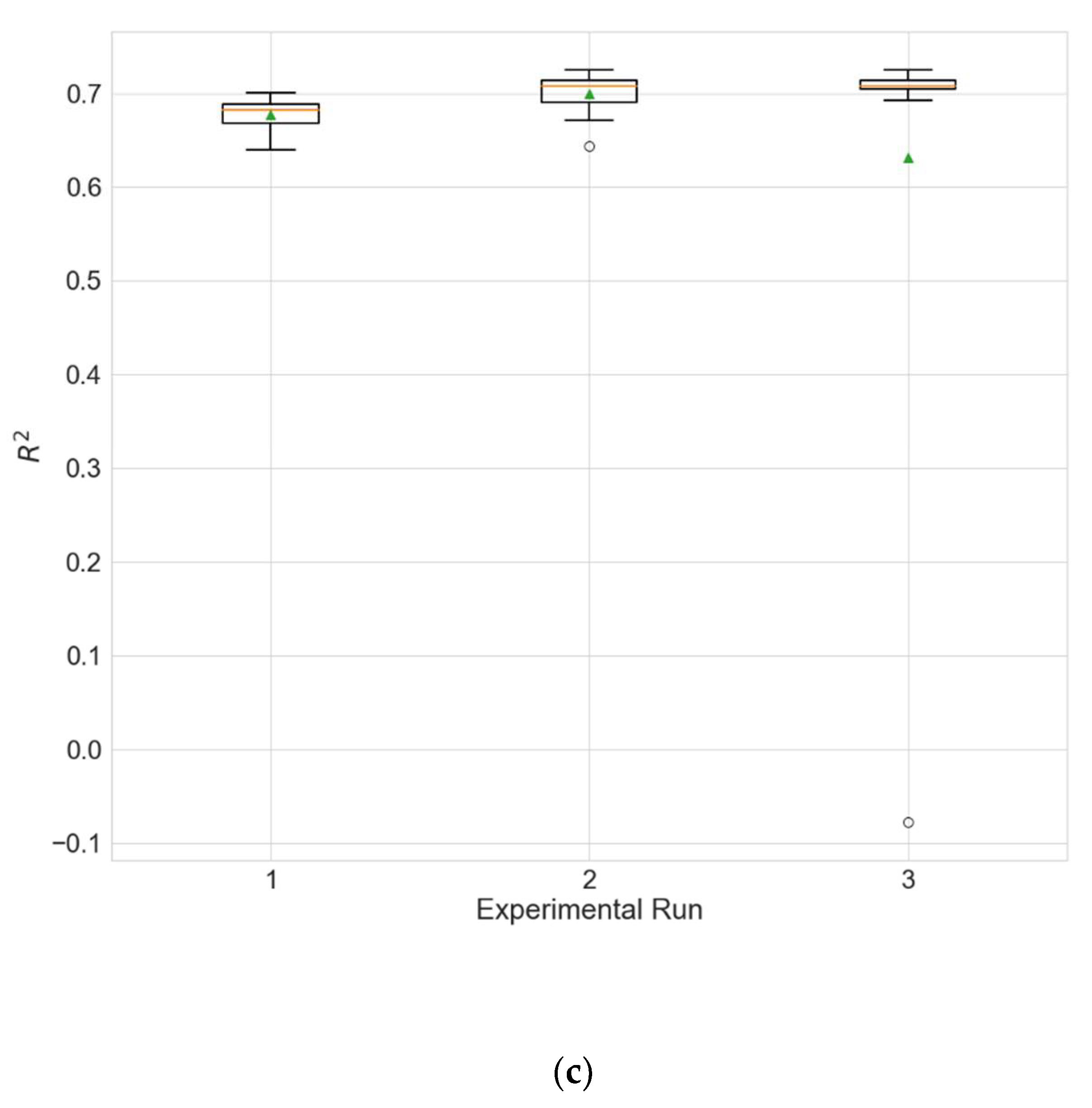
In order to evaluate whether the selection of input variables by random searching leads to improved model performance, two additional experiments are accomplished. In the first experiment, the models use only PM_2.5 as input, and in the second experiment all 12 available variables are used as input. The results of these two experiments are given in Table 23 and Table 24. Figure 9 and Figure 10 show the distributions of the different performance metrics as boxplots. As can be seen, the employment of additional variables besides the historical data of the predicted variable (PM_2.5 in this case) improves the performance of the model (p much less than 0.05 for all metrics).

Table 23. Performance of the best architecture for station Wanliu for each experimental run, using only PM_2.5 as input. The values are averaged over the 10 independent training runs.

Run	MAE	RMSE	R2
1	18.418 ± 0.248	29.895 ± 0.500	0.865 ± 0.004
2	17.893 ± 0.361	29.144 ± 0.557	0.872 ± 0.005
3	18.255 ± 0.262	30.830 ± 0.506	0.856 ± 0.005

Table 24. Performance of the best architecture for station Wanliu for each experimental run, using all variables as input. The values are averaged over the 10 independent training runs.

Run	MAE	RMSE	R2
1	15.189 ± 0.524	24.630 ± 1.196	0.908 ± 0.009
2	15.376 ± 0.660	25.593 ± 2.263	0.900 ± 0.019
3	16.183 ± 0.333	27.641 ± 1.010	0.885 ± 0.009

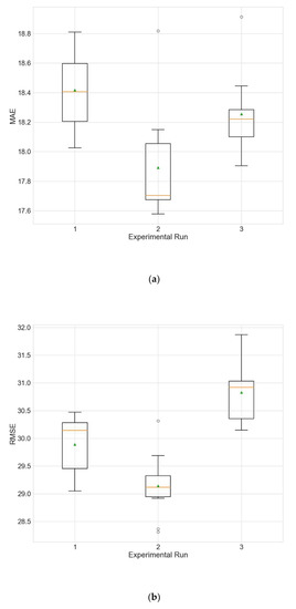
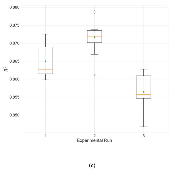
Figure 9. Boxplot showing the distributions of the different performance metrics of the best architecture for station Wanliu from the experiment that that uses only PM_2.5 as input. (a) MAE; (b) RMSE; (c) R².

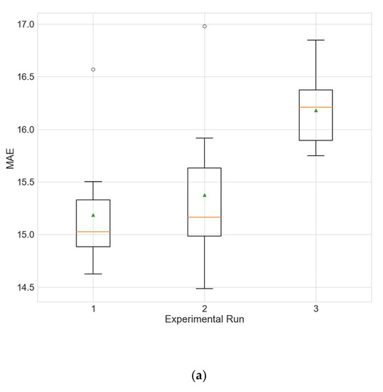
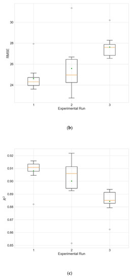
Figure 10. Boxplot showing the distributions of the different performance metrics of the best architecture for station Wanliu from the experiment that uses all variables as input. (a) MAE; (b) RMSE; (c) R².

The use of all variables produces similar results to those in the main experiment (Table 4) (p > 0.5 for all metrics), but the full training of the models takes a significantly longer time (p = 2.28 × 10⁻⁰⁷, one full training when using all variables takes an average of 1.84 h compared to an average of 0.84 h when the input variables are selected by random search).

4.6. Inclusion of Spatial Information

In order to evaluate the influence of the inclusion of spatial information on the performance of the model, an experiment is carried out in which models with a fixed neighborhood size of 0 are evolved, i.e., data from other neighboring stations are not taken into account, and only data from the target station are used. The results are given in Table 25, and the comparison with the results of the main experiment (Table 4) confirms that the inclusion of spatial information significantly improves the performance of the model (p much less than 0.05 for all metrics). Figure 11 shows the distributions of the different performance metrics as a boxplot.

Table 25. Performance of the best architecture for station Wanliu for each experimental run using a fixed neighborhood size of 0. The values are averaged over the 10 independent training runs.

Run	MAE	RMSE	R2
1	26.036 ± 0.625	46.205 ± 1.175	0.678 ± 0.017
2	24.929 ± 0.799	44.611 ± 1.751	0.699 ± 0.024
3	27.234 ± 9.189	47.903 ± 12.218	0.631 ± 0.237

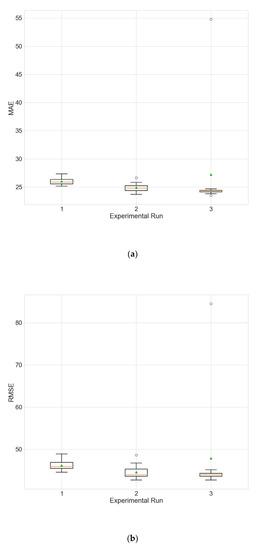
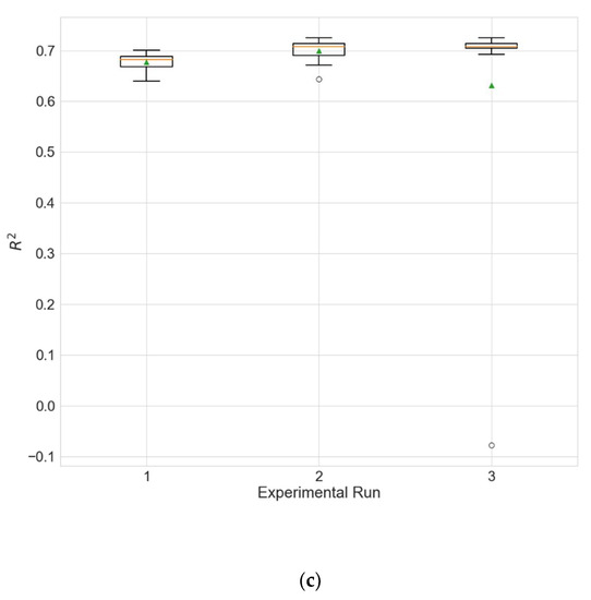
Figure 11. Boxplot showing the distributions of the different performance metrics of the best architecture for station Wanliu from the experiment that uses a fixed neighborhood size of 0. (a) MAE; (b) RMSE; (c) R².

5. Conclusions

Air pollution has a negative impact on human health and the environment, thus necessitating the development of effective air quality forecasting systems that would allow appropriate measures to be taken in a timely manner.

The suggested deep spatiotemporal model for predicting air pollution with the automatic selection of input variables uses a genetic algorithm for the optimization of network architecture and hyperparameters. In addition, a hybrid strategy for filling in the missing values in time series is proposed. The experimental evaluation using a publicly available data set demonstrates that even with limited computational resources, the evolved architectures provide good and consistent results. The inclusion of the trained models in different ensembles further improves the results, bringing them closer to those obtained with some modern deep models using the same data set, and in some cases even showing superior performance.

The hybrid strategy for missing value imputation has advantages over linear interpolation, especially for data with very clear seasonality, without lagging behind in many other cases. The experimental results also reveal that random searching is a simple and effective strategy for selecting the input variables. Moreover, the inclusion of spatial information significantly improves the predictive results obtained with the models.

Future work will be aimed at improving the spatial component of the model by making the size of the neighborhood window dynamic and dependent on the local meteorological conditions.

References

- Kampa, M.; Castanas, E. Human health effects of air pollution. Environ. Pollut. 2008, 151, 362–367. [Google Scholar] [CrossRef] [PubMed]
- Kim, K.H.; Kabir, E.; Kabir, S. A review on the human health impact of airborne particulate matter. Environ. Int. 2015, 74, 136–143. [Google Scholar] [CrossRef] [PubMed]
- World Health Organization. Regional Office for Europe. Review of Evidence on Health Aspects of Air Pollution: REVIHAAP. Project: Technical Report. 2021. Available online: https://apps.who.int/iris/handle/10665/341712 (accessed on 21 April 2022).
- Lippmann, M. Toxicological and epidemiological studies of cardiovascular effects of ambient air fine particulate matter (PM2.5) and its chemical components: Coherence and public health implications. Crit. Rev. Toxicol. 2014, 44, 299–347. [Google Scholar] [CrossRef] [PubMed]
- Xing, Y.F.; Xu, Y.H.; Shi, M.H.; Lian, Y.X. The impact of PM2.5 on the human respiratory system. J. Thorac. Dis. 2016, 8, E69–E74. [Google Scholar]
- Bu, X.; Xie, Z.; Liu, J.; Wei, L.; Wang, X.; Chen, M.; Ren, H. Global PM2.5-attributable health burden from 1990 to 2017: Estimates from the global burden of disease study 2017. Environ. Res. 2021, 197, 111123. [Google Scholar] [CrossRef]
- Apte, J.S.; Brauer, M.; Cohen, A.J.; Ezzati, M.; Pope, C.A., III. Ambient PM2.5 reduces global and regional life expectancy. Environ. Sci. Technol. Lett. 2018, 5, 546–551. [Google Scholar] [CrossRef] [Green Version]
- Yin, H.; Brauer, M.; Zhang, J.J.; Cai, W.; Navrud, S.; Burnett, R.; Howard, C.; Deng, Z.; Kammen, D.M.; Schellnhuber, H.J.; et al. Population ageing and deaths attributable to ambient PM2.5 pollution: A global analysis of economic cost. Lancet Planet. Health 2021, 5, e356–e367. [Google Scholar] [CrossRef]
- Zhang, Y.; Bocquet, M.; Mallet, V.; Seigneur, C.; Baklanov, A. Real-time air quality forecasting, part I: History, techniques, and current status. Atmos. Environ. 2012, 60, 632–655. [Google Scholar] [CrossRef]
- Grell, G.A.; Peckham, S.E.; Schmitz, R.; McKeen, S.A.; Frost, G.; Skamarock, W.C.; Eder, B. Fully coupled “online” chemistry within the WRF model. Atmos. Environ. 2005, 39, 6957–6975. [Google Scholar] [CrossRef]
- Byun, D.; Schere, K.L. Review of the governing equations, computational algorithms, and other components of the Models-3 Community Multiscale Air Quality (CMAQ) modeling system. Appl. Mech. Rev. 2006, 59, 51–77. [Google Scholar] [CrossRef]
- Appel, K.W.; Bash, J.O.; Fahey, K.M.; Foley, K.M.; Gilliam, R.C.; Hogrefe, C.; Hutzell, W.T.; Kang, D.; Mathur, R.; Murphy, B.N.; et al. The Community Multiscale Air Quality (CMAQ) model versions 5.3 and 5.3.1: System updates and evaluation. Geosci. Model Dev. 2021, 14, 2867–2897. [Google Scholar] [CrossRef] [PubMed]
- Menut, L.; Bessagnet, B.; Khvorostyanov, D.; Beekmann, M.; Blond, N.; Colette, A.; Coll, I.; Curci, G.; Foret, G.; Hodzic, A.; et al. CHIMERE 2013: A model for regional atmospheric composition modelling. Geosci. Model Dev. 2013, 6, 981–1028. [Google Scholar] [CrossRef] [Green Version]
- Mailler, S.; Menut, L.; Khvorostyanov, D.; Valari, M.; Couvidat, F.; Siour, G.; Turquety, S.; Briant, R.; Tuccella, P.; Bessagnet, B.; et al. CHIMERE-2017: From urban to hemispheric chemistry-transport modeling. Geosci. Model Dev. 2017, 10, 2397–2423. [Google Scholar] [CrossRef] [Green Version]
- Menut, L.; Bessagnet, B.; Briant, R.; Cholakian, A.; Couvidat, F.; Mailler, S.; Pennel, R.; Siour, G.; Tuccella, P.; Turquety, S.; et al. The CHIMERE v2020r1 online chemistry-transport model. Geosci. Model Dev. 2021, 14, 6781–6811. [Google Scholar] [CrossRef]
- Abderrahim, H.; Chellali, M.R.; Hamou, A. Forecasting PM10 in Algiers: Efficacy of multilayer perceptron networks. Environ. Sci. Pollut. Res. 2016, 23, 1634–1641. [Google Scholar] [CrossRef] [PubMed]
- Dedovic, M.M.; Avdakovic, S.; Turkovic, I.; Dautbasic, N.; Konjic, T. Forecasting PM10 Concentrations Using Neural Networks and System for Improving Air Quality. In Proceedings of the XI International Symposium on Telecommunications (BIHTEL), Sarajevo, Bosnia and Herzegovina, 24–26 October 2016; pp. 1–6. [Google Scholar]
- Masood, A.; Ahmad, K. A model for particulate matter (PM2.5) prediction for Delhi based on machine learning approaches. Procedia Comput. Sci. 2020, 167, 2101–2110. [Google Scholar] [CrossRef]
- Mechgoug, R.; Ahmed, A.T.; Cherroun, L. Optimization of Neural Predictor for Air Pollution. In Proceedings of the World Congress on Engineering, London, UK, 4–6 July 2012; Volume 2, pp. 370–377. [Google Scholar]
- Moustris, K.P.; Ziomas, I.C.; Paliatsos, A.G. 3-Day-ahead forecasting of regional pollution index for the pollutants NO2, CO, SO2, and O3 using artificial neural networks in Athens, Greece. Water Air Soil Pollut. 2010, 209, 29–43. [Google Scholar] [CrossRef]
- Moustris, K.; Larissi, I.; Nastos, P.T.; Koukouletsos, K.; Paliatsos, A.G. 24-Hours Ahead Forecasting of PM10 Concentrations Using Artificial Neural Networks in the Greater Athens Area, Greece. In Advances in Meteorology, Climatology and Atmospheric Physics; Helmis, C.G., Nastos, P.T., Eds.; Springer: Berlin/Heidelberg, Germany, 2012; Volume 2, pp. 1121–1126. [Google Scholar]
- Pasero, E.; Mesin, L. Artificial Neural Networks to Forecast Air Pollution. In Air Pollution; Villanyi, V., Ed.; InTech Open: London, UK, 2010; pp. 221–240. [Google Scholar]
- Skrzypski, J.; Jach-Szakiel, E. Neural network prediction models as a tool for air quality management in cities. Environ. Prot. Eng. 2008, 34, 129–137. [Google Scholar]
- Unnikrishnan, R.; Madhu, G. Comparative study on the effects of meteorological and pollutant parameters on ANN modelling for prediction of SO2. SN Appl. Sci. 2019, 1, 1394. [Google Scholar] [CrossRef] [Green Version]
- Awang, N.R.; Ramli, N.A.; Yahaya, A.S.; Elbayoumi, M. Multivariate methods to predict ground level ozone during daytime, nighttime, and critical conversion time in urban areas. Atmos. Pollut. Res. 2015, 6, 726–734. [Google Scholar] [CrossRef]
- Zhang, L.; Lin, J.; Qiu, R.; Hu, X.; Zhang, H.; Chen, Q.; Tan, H.; Lin, D.; Wang, J. Trend analysis and forecast of PM2.5 in Fuzhou, China using the ARIMA model. Ecol. Indic. 2018, 95, 702–710. [Google Scholar] [CrossRef]
- Li, X.; Luo, A.; Li, J.; Li, Y. Air pollutant concentration forecast based on support vector regression and quantum-behaved particle swarm optimization. Environ. Modeling Assess. 2019, 24, 205–222. [Google Scholar] [CrossRef]
- Lv, B.; Cobourn, W.G.; Bai, Y. Development of nonlinear empirical models to forecast daily PM2.5 and ozone levels in three large Chinese cities. Atmos. Environ. 2016, 147, 209–223. [Google Scholar] [CrossRef]
- Chen, G.; Li, S.; Knibbs, L.D.; Hamm, N.A.; Cao, W.; Li, T.; Guo, J.; Ren, H.; Abramson, M.J.; Guo, Y. A machine learning method to estimate PM2.5 concentrations across China with remote sensing, meteorological and land use information. Sci. Total Environ. 2018, 636, 52–60. [Google Scholar] [CrossRef] [PubMed]
- Greff, K.; Srivastava, R.K.; Koutník, J.; Steunebrink, B.R.; Schmidhuber, J. LSTM: A search space odyssey. IEEE Trans. Neural Netw. Learn. Syst. 2016, 28, 2222–2232. [Google Scholar] [CrossRef] [PubMed] [Green Version]
- Alsaedi, A.S.; Liyakathunisa, L. Spatial and Temporal Data Analysis with Deep Learning for Air Quality Prediction. In Proceedings of the 12th International Conference on Developments in eSystems Engineering (DeSE), Kazan, Russia, 7–10 October 2019; pp. 581–587. [Google Scholar]
- Ao, D.; Cui, Z.; Gu, D. Hybrid Model of air Quality Prediction Using K-Means Clustering and Deep Neural Network. In Proceedings of the Chinese Control Conference (CCC), Guangzhou, China, 27–30 July 2019; pp. 8416–8421. [Google Scholar]
- Garg, S.; Jindal, H. Evaluation of Time Series Forecasting Models for Estimation of PM2.5 Levels in Air. In In Proceedings of the 6th International Conference for Convergence in Technology (I2CT), Maharashtra, India, 2–4 April 2021; pp. 1–8. [Google Scholar]
- Gul, S.; Khan, G.M. Forecasting Hazard Level of Air Pollutants Using LSTM’s. In Artificial Intelligence Applications and Innovations. AIAI 2020. IFIP Advances in Information and Communication Technology; Maglogiannis, I., Iliadis, L., Pimenidis, E., Eds.; Springer: Cham, Switzerland, 2020; Volume 584, pp. 143–153. [Google Scholar]
- Kök, İ.; Şimşek, M.U.; Özdemir, S. A Deep Learning Model for Air Quality Prediction in Smart Cities. In Proceedings of the IEEE International Conference on Big Data, Boston, MA, USA, 11–14 December 2017; pp. 1983–1990. [Google Scholar]
- Tsai, Y.T.; Zeng, Y.R.; Chang, Y.S. Air Pollution Forecasting Using RNN with LSTM. In Proceedings of the 4th IEEE International Conference on Big Data Intelligence and Computing, Athens, Greece, 12–15 August 2018; pp. 1074–1079. [Google Scholar]
- Lecun, Y.; Bottou, L.; Bengio, Y.; Haffner, P. Gradient-based learning applied to document recognition. Proc. IEEE 1998, 86, 2278–2324. [Google Scholar] [CrossRef] [Green Version]
- Kow, P.Y.; Wang, Y.S.; Zhou, Y.; Kao, I.F.; Issermann, M.; Chang, L.C.; Chang, F.J. Seamless integration of convolutional and back-propagation neural networks for regional multi-step-ahead PM2.5 forecasting. J. Clean. Prod. 2020, 261, 121285. [Google Scholar] [CrossRef]
- Du, S.; Li, T.; Yang, Y.; Horng, S.J. Deep air quality forecasting using hybrid deep learning framework. IEEE Trans. Knowl. Data Eng. 2021, 33, 2412–2424. [Google Scholar] [CrossRef] [Green Version]
- Huang, C.-J.; Kuo, P.-H. A deep CNN-LSTM model for particulate matter (PM2.5) forecasting in smart cities. Sensors 2018, 18, 2220. [Google Scholar] [CrossRef] [Green Version]
- Pak, U.; Kim, C.; Ryu, U.; Sok, K.; Pak, S. A hybrid model based on convolutional neural networks and long short-term memory for ozone concentration prediction. Air Qual. Atmos. Health 2018, 11, 883–895. [Google Scholar] [CrossRef]
- Wardana, I.; Gardner, J.W.; Fahmy, S.A. Optimising Deep Learning at the Edge for Accurate Hourly Air Quality Prediction. Sensors 2021, 21, 1064. [Google Scholar] [CrossRef] [PubMed]
- Wen, C.; Liu, S.; Yao, X.; Peng, L.; Li, X.; Hu, Y.; Chi, T. A novel spatiotemporal convolutional long short-term neural network for air pollution prediction. Sci. Total Environ. 2019, 654, 1091–1099. [Google Scholar] [CrossRef] [PubMed]
- Junninen, H.; Niska, H.; Tuppurainen, K.; Ruuskanen, J.; Kolehmainen, M. Methods for imputation of missing values in air quality data sets. Atmos. Environ. 2004, 38, 2895–2907. [Google Scholar] [CrossRef]
- Galelli, S.; Humphrey, G.B.; Maier, H.R.; Castelletti, A.; Dandy, G.C.; Gibbs, M.S. An evaluation framework for input variable selection algorithms for environmental data-driven models. Environ. Model. Softw. 2014, 62, 33–51. [Google Scholar] [CrossRef] [Green Version]
- Kadkhodazadeh, M.; Valikhan Anaraki, M.; Morshed-Bozorgdel, A.; Farzin, S. A new methodology for reference evapotranspiration prediction and uncertainty analysis under climate change conditions based on machine learning, multi criteria decision making and Monte Carlo methods. Sustainability 2022, 14, 2601. [Google Scholar] [CrossRef]
- Kadkhodazadeh, M.; Farzin, S. A Novel LSSVM Model Integrated with GBO Algorithm to Assessment of Water Quality Parameters. Water Resour. Manag. 2021, 35, 3939–3968. [Google Scholar] [CrossRef]
- Fan, J.; Li, Q.; Hou, J.; Feng, X.; Karimian, H.; Lin, S. A spatiotemporal prediction framework for air pollution based on deep RNN. ISPRS Ann. Photogramm. Remote Sens. Spat. Inf. Sci. 2017, IV-4/W2, 15–22. [Google Scholar] [CrossRef] [Green Version]
- Wang, Y.; Liu, P.; Xu, C.; Peng, C.; Wu, J. A deep learning approach to real-time CO concentration prediction at signalized intersection. Atmos. Pollut. Res. 2020, 11, 1370–1378. [Google Scholar] [CrossRef]
- Photphanloet, C.; Lipikorn, R. PM10 concentration forecast using modified depth-first search and supervised learning neural network. Sci. Total Environ. 2020, 727, 138507. [Google Scholar] [CrossRef]
- Zhao, H.; Zhang, J.; Wang, K.; Bai, Z.; Liu, A. A GA-ANN Model for Air Quality Predicting. In Proceedings of the International Computer Symposium, Tainan, Taiwan, 16–18 December 2010; pp. 693–699. [Google Scholar]
- Ghoneim, O.A.; Manjunatha, B.R. Forecasting of Ozone Concentration in Smart City Using Deep Learning. In Proceedings of the International Conference on Advances in Computing, Communications and Informatics, Udupi, India, 13–16 September 2017; pp. 1320–1326. [Google Scholar]
- Kapageridis, I.; Triantafyllou, A.G. A genetically optimised neural network for prediction of maximum hourly PM10 concentration. WIT Trans. Ecol. Environ. 2004, 74, 161–170. [Google Scholar]
- Wang, H.W.; Li, X.B.; Wang, D.; Zhao, J.; He, H.; Peng, Z.R. Regional prediction of ground-level ozone using a hybrid sequence-to-sequence deep learning approach. J. Clean. Prod. 2020, 253, 119841. [Google Scholar] [CrossRef]
- Perez, P.; Gramsch, E. Forecasting hourly PM2.5 in Santiago de Chile with emphasis on night episodes. Atmos. Environ. 2016, 124, 22–27. [Google Scholar] [CrossRef]
- Zhao, J.; Deng, F.; Cai, Y.; Chen, J. Long short-term memory-Fully connected (LSTM-FC) neural network for PM2.5 concentration prediction. Chemosphere 2019, 220, 486–492. [Google Scholar] [CrossRef] [PubMed]
- Wang, J.; Song, G. A deep spatial-temporal ensemble model for air quality prediction. Neurocomputing 2018, 314, 198–206. [Google Scholar] [CrossRef]
- Soh, P.W.; Chang, J.W.; Huang, J.W. Adaptive deep learning-based air quality prediction model using the most relevant spatial-temporal relations. IEEE Access 2018, 6, 38186–38199. [Google Scholar] [CrossRef]
- Zheng, Y.; Yi, X.; Li, M.; Li, R.; Shan, Z.; Chang, E.; Li, T. Forecasting Fine-Grained Air Quality Based on Big Data. In Proceedings of the 21th ACM SIGKDD International Conference on Knowledge Discovery and Data Mining, Sydney, Australia, 10–13 August 2015; pp. 2267–2276. [Google Scholar]
- Zou, X.; Zhao, J.; Zhao, D.; Sun, B.; He, Y.; Fuentes, S. Air quality prediction based on a spatiotemporal attention mechanism. Mob. Inf. Syst. 2021, 2021, 6630944. [Google Scholar] [CrossRef]
- Yosifov, G.; Petrov, M. Traffic Flow City Index Based on Public Transportation Vehicles Data. In Proceedings of the 21st International Conference on Computer Systems and Technologies’ 20, Ruse, Bulgaria, 19–20 June 2020; pp. 201–207. [Google Scholar]
- Li, X.; Peng, L.; Yao, X.; Cui, S.; Hu, Y.; You, C.; Chi, T. Long short-term memory neural network for air pollutant concentration predictions: Method development and evaluation. Environ. Pollut. 2017, 231, 997–1004. [Google Scholar] [CrossRef]
- Zhang, S.; Guo, B.; Dong, A.; He, J.; Xu, Z.; Chen, S.X. Cautionary tales on air-quality improvement in Beijing. Proc. R. Soc. A Math. Phys. Eng. Sci. 2017, 473, 20170457. [Google Scholar] [CrossRef] [PubMed] [Green Version]
- Ghosh, P.; Neufeld, A.; Sahoo, J.K. Forecasting directional movements of stock prices for intraday trading using LSTM and random forests. Financ. Res. Lett. 2021, 46, 102280. [Google Scholar] [CrossRef]
- Pedregosa, F.; Varoquaux, G.; Gramfort, A.; Michel, V.; Thirion, B.; Grisel, O.; Blondel, M.; Prettenhofer, P.; Weiss, R.; Dubourg, V.; et al. Scikit-learn: Machine learning in Python. J. Mach. Learn. Res. 2011, 12, 2825–2830. [Google Scholar]
- Tsokov, S.; Lazarova, M.; Aleksieva-Petrova, A. An evolutionary approach to the design of convolutional neural networks for human activity recognition. Indian J. Comput. Sci. Eng. 2021, 12, 499–517. [Google Scholar] [CrossRef]
- Tsokov, S.; Lazarova, M.; Aleksieva-Petrova, A. A Novel Biologically Inspired Developmental Indirect Encoding for the Evolution of Neural Network Controllers for Autonomous Agents. In Proceedings of the Technical University of Sofia; Technical University of Sofia: Sofia, Bulgaria, 2021; Volume 71, pp. 23–29. [Google Scholar]
Publisher’s Note: MDPI stays neutral with regard to jurisdictional claims in published maps and institutional affiliations. |
© 2022 by the authors. Licensee MDPI, Basel, Switzerland. This article is an open access article distributed under the terms and conditions of the Creative Commons Attribution (CC BY) license (https://creativecommons.org/licenses/by/4.0/).