Abstract
With the rapid development of Industrial 4.0, the modern manufacturing system has been experiencing profoundly digital transformation. The development of new technologies helps to improve the efficiency of production and the quality of products. However, for the increasingly complex production systems, operational decision making encounters more challenges in terms of having sustainable manufacturing to satisfy customers and markets’ rapidly changing demands. Nowadays, rule-based heuristic approaches are widely used for scheduling management in production systems, which, however, significantly depends on the expert domain knowledge. In this way, the efficiency of decision making could not be guaranteed nor meet the dynamic scheduling requirement in the job-shop manufacturing environment. In this study, we propose using deep reinforcement learning (DRL) methods to tackle the dynamic scheduling problem in the job-shop manufacturing system with unexpected machine failure. The proximal policy optimization (PPO) algorithm was used in the DRL framework to accelerate the learning process and improve performance. The proposed method was testified within a real-world dynamic production environment, and it performs better compared with the state-of-the-art methods.
1. Introduction
With the rapid development of automation and digitization, Industry 4.0 signifies a remarkable shift in industrial revolution [1,2]. As a practical application of manufacturing in the Industry 4.0 era, smart factories are presented through the leverage of new technologies, including the Internet of Things (IoTs) and artificial intelligence (AI) [3,4]. Through the full interconnection between the digital and the physical world, smart factories can realize sustainable development that significantly improves productivity and quality [5]. Sustainability has been proposed as the economic indicator to evaluate sustainable practices in the manufacturing sector [6,7,8]. In today’s globalized market, manufacturing industries need to deploy strategy, demanding that it could continuously maintain high efficiency, competitiveness, and sustainability [9]. There are several factors that could affect the sustainability of manufactured products, such as the supplement of raw materials, stability and efficiency of production processes, and distribution capability [10].
As the smart production system becomes increasingly complicated, operation decision making has become more and more important for keeping sustainable working and production efficiency [11,12]. Many factors can seriously affect the utilization and sustainability of production lines. For instance, the rapidly changing market needs and unexpected machine failures can significantly reduce the efficiency and performance of the production system [13]. For the complex job-shop manufacturing system, the job-shop scheduling problem becomes one of the most important production scheduling problems in smart manufacturing areas. The scheduling optimization approaches can improve the sustainable production of manufacturing enterprises as well as their market competitiveness [14,15].
The job-shop scheduling problem is a combinatorial optimization problem related to scheduling and production control, which aims to identify the optimal sequential and process order of the jobs in the manufacturing industry [16,17]. It can be analyzed as a nondeterministic polynomial hard (NP-hard) problem when there are two or more machines involved [18]. Generally, heuristic-based methods are the main way to solve job-shop scheduling, including linear programming approaches [19], simulated annealing algorithm [20], genetic algorithm [21], particle swarm optimization [22], and teaching–learning-based optimization [23]. These approaches can obtain the optimal solution under certain conditions. However, they do not have the ability to deal with the dynamic job-shop environment with uncertainties [24]. Combining advanced AI and data-driven approaches, the dynamic job-shop scheduling methods are proposed to handle the uncertain factors and dynamic environments of smart manufacturing, which allow both real-time production scheduling and dynamic adaptive production scheduling [25,26,27]. Nowadays, more and more data-driven AI methods have been proposed to tackle the dynamic scheduling problem for job-shop manufacturing systems [28,29,30].
The dynamic job-shop scheduling problem is difficult to solve by the typical heuristics method due to the existing dynamic events such as random ordering arrivals and unexpected machine breakdowns. To deal with this issue, the deep reinforcement learning (DRL) method was proposed to combine deep learning and reinforcement learning methods [31,32,33,34]. DRL can formulate scheduling strategies based on real-time production data and optimize strategies according to the dynamic changes of the system states. In the actual scenarios of smart manufacturing, the job-shop environment can apply sensory technologies to detect and collect large amounts of production process data. Through processing and training the real-time data of the job-shop environment states, valuable scheduling information and policy can be learned for dynamic optimizing the scheduling. Zhao et al. proposed the deep Q-network (DQN) to improve the performance of the adaptive scheduling algorithm in dynamic smart manufacturing [35]. Wang et al. [36] and Zeng et al. [37] proposed the dual Q-learning (D-Q) method as the solution of the dynamic job-shop scheduling problem. Luo et al. [38] proposed a two-hierarchy deep Q-network to deal with flexible job-shop scheduling problems with the disturbance of new jobs. The DRL method has become one of the dominant methods in dealing with the dynamic job-shop scheduling problem. However, all the mentioned DRL methods are constructed based on the designed rules, which means the learned agent is used to select the optimal scheduling rule, and they did not involve the machine failure situation. There are very few studies that could directly control the raw actions of agents to schedule the dynamic job-shop manufacturing system with unexpected machine failure.
To tackle these challenges, we propose a deep reinforcement learning framework under the proximal policy optimization (PPO) algorithm for addressing the dynamic scheduling problem of a designed job-shop manufacturing system with unexpected machine failure. Different from previous works, our method continuously outputs the raw actions that keep the production system sustainable, working and producing the products with high efficiency even under the unexpected machine failure situation. Compared with different policy gradient methods, we select the PPO algorithm that has a stable learning process and fast optimization speed. Different reward functions were designed and tested to guide the dispatcher agent in learning varying policies.
2. Preliminary
In this section, we briefly describe the fundamental theory of policy gradient-based reinforcement learning, which we proposed to use for the dynamic job-shop scheduling problem.
2.1. Markov Decision Process
The Markov decision process (MDP) is the idealized mathematical formulation of reinforcement learning [39] with the control problem, which consists of a state space S, an action space A, a state transition probability distribution , and a reward function . The RL aims at training an agent with policy to act in a certain environment and maximize the cumulative rewards coming from the selected actions across the sequence of time. The actions are determined based on the policy in each time step, and a trajectory of states, actions, and rewards, from can be obtained by the agent using its policy to interact with the environment. The purpose of the agent is to learn a policy that can maximize the cumulative discounted rewards from the state–action pair:
where the return is the total discounted reward , and is the discount factor.
2.2. Policy Gradient Theorem
For the continuous control problem of the reinforcement learning, we usually use the policy gradient method to maximize the expected total reward. The fundamental idea of this algorithm is to train the policy with the parameter by utilizing the stochastic gradient descent algorithm with the objective function:
where represents the integration of the variables; the states and actions are sampled from the dynamics model and policy , as is explained in the MDP; and denotes the sum of expected rewards which is the value function in practice. So, we can consider that the Equation (2) consists of the policy gradient and the cumulative rewards, and the direction of the gradient is significantly related to . Previous studies [40] have been conducted to explore the approaches of approximating the total expected rewards , and there are several formulations in the discounted way for variance reduction:
The advantage function, , is used for assessing whether the action is better or worse than the policy’s default behavior. Since the advantage function has the lowest variance in the process of policy promotion, should choose the advantage function , so that the objective function can provide the direction of advance only if .
3. Proposed Methods
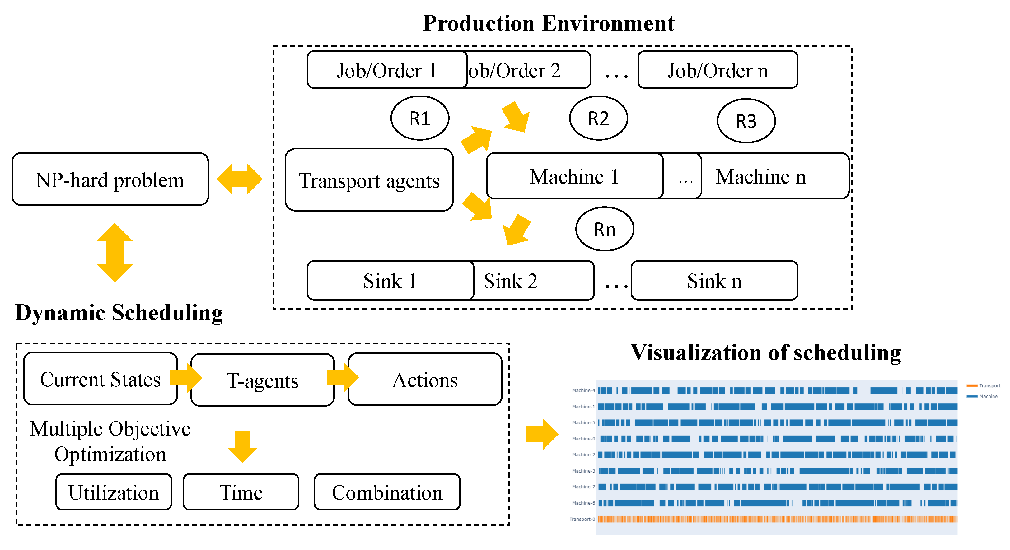
Figure 1 shows an overview of the proposed dynamic job-shop scheduling approach. This problem is a typical NP-hard problem and its computational complexity significantly increases with the number of elements in the environment [18,19]. In the production environment, the transport agents take the jobs or orders to the machines, then the production is generated from the machine in order to be transported to the sink waiting for delivery to the next processing station. The transport agents should determine the next actions based on the current state of the environment. The multiple objective functions should be considered to increase production efficiency, such as increasing the utilization of machines and reducing order waiting time and their combinations. The dynamic environment can be affected by certain random events, such as machine breakdown, resource cut off, etc. The dynamic scheduling should maintain the production system operating at high-efficiency conditions so that the stakeholders are able to save more costs when unexpected random events happen.

Figure 1.
The overview of dynamic job-shop scheduling.
3.1. Dynamic Simulation of Production Environment
The simulation environment of job-shop manufacturing production constitutes the foundation of the proposed method. The agent is trained with a large amount of historical data, which are the outcome of interacting with the dynamic simulation [34]. The intelligent scheduling strategy was explored during the interaction procedure and recorded in the agent model.
As shown in Figure 1, the input of the simulated production system is ordered, and the entry resource is called Source. Machine is responsible for processing orders, then the disposed orders are transported to the resource called Sink. The critical resource called Dispatcher is going to transport the order between Source, Machine, and Sink. Therefore, there are three states for each order, including waiting, intransport, and inprocess. When the order is in the waiting state, it should be put in one of the buffers. There are entrance and exit buffers for each machine, which are used to receive undisposed orders and store the disposed of orders, respectively.
The constraints of the real-world production system are considered in this dynamic simulation environment, making it similar to the real-world application.
- Machines that have similar disposal ability of orders are put into the same group.
- Orders are released by the sources and they are performed according to specific probability.
- The processing time of each order is decided by the predefined probability distribution.
- Machine failures are considered in this environment, which can result in the breakdown of all of the machines. The failure events are random triggered based on the mean time between failure (MTBF) and mean time off-line (MTOL).
3.1.1. Action Module
The transport agent is the most important in the dynamic environment because it dispatches all orders from the source to machine and machine to sink. It is called the dispatcher in this work. Accordingly, there are three types of actions, i.e., , , and , as shown in Table 1.

Table 1.
Action Type.
The actions of and belong to executable actions . At every time step, the dispatcher selects an action. However, not every could be performed. It would be relying on the states of current production. For instance, an action could be valid only if the source has a new order while the machine has a free buffer and they are working at normal function and capable of processing it. Therefore, the action could be determined as either valid or invalid at each time step. If the transport agent successively selects the invalid action when it is repeated up to a maximum recursion count, the is performed.
3.1.2. States
The states are the current observations from the production environment, which are the outcome of previous actions. The agent can determine the next action based on the historical and current states. Ideally, the state contains all the information both related and unrelated to the production process. However, an excess of unrelated states can increase the dimension of solution space, which leads to a significant decline in the performance. Therefore, the states in this simulation environment are carefully designed and could synchronize with the real-world system. Each element in the states can be calculated at the current time t, and we neglect the t for better readability.
- Firstly, the state of action shows whether the current action is valid or not, and it is defined as:
- The machine breakdown was designed in the simulation, and the state of failure for each machine is also considered, which is defined as:
- The remaining processing time of each machine is defined as:where is the remaining processing time, and is the average processing time at .
- indicates the state information of remaining free buffer spaces of each machine in its entry buffer:where is the number of occupied buffers, and is the capacity of the entry buffer.
- indicates the remaining free buffer space in the exit buffer for each machine :where is the number of occupied buffers, and is the capacity of the exit buffer.
- indicates the waiting times of orders waiting for transport:where is the longest waiting time, and and are the average and standard variation of waiting time of orders.
3.2. Deep Reinforcement Learning for Dynamic Scheduling
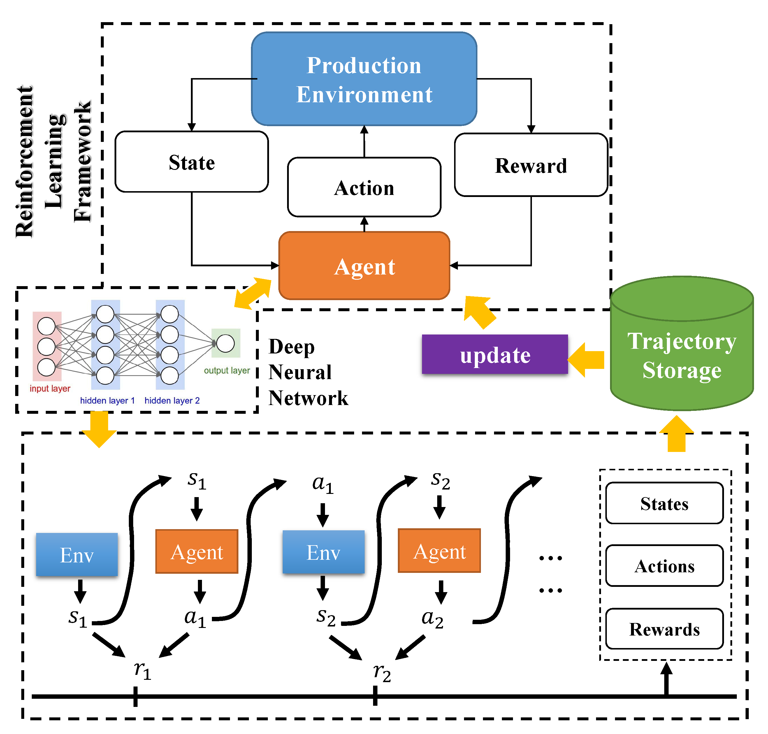
The framework of deep reinforcement learning for the dynamic scheduling problem is shown in Figure 2. The initial dispatcher agent interacts with the simulation of the production environment randomly. Then, the inside policy of the agent is optimized using certain periods of trajectories including the state, action, and the reward of each time t. The intelligent policy is explored at the interaction procedure, and the deep neural network records and transfers them as the parameters. Following the foundation of MDP, the DRL method aims at obtaining a long period of rewards. It is obvious that the proposed method should be more suitable for the dynamic scheduling problem than the general method, such as FIFO and NJF [41], which make decisions depending on the current states.

Figure 2.
Deep reinforcement learning framework for dynamic scheduling problem.
3.2.1. Optimization Objectives
As shown in Figure 2, to continuously perform the expected actions that meet the designed requirements, the DRL agent need to receive the rewards at each time step. Following the MDP, it is obvious that the DRL agent not only considers the best action at present but also aims at acquiring good performance in the long-term period. As the multiple objective optimization, there are two objectives in the proposed production environment, including average utilization of the machines and average waiting time of orders.
- The constant reward rewards the valid action with value for , and for is defined as:
- To promote the average utilization U, was designed with exponential function when the agent provides a valid action. The purpose of this reward function is to maximize utilization, and it is defined as:
- To shorten the waiting time of orders, is designed to award the valid action determined by the agent. The reward function also follows the exponential function to accelerate the order leaving the system, which is defined as:
- Combining with and , two complex reward functions are designed as follows:
- For implementing the multiple-objective optimization, the hybrid reward function with and is defined as:
3.2.2. Proximal Policy Optimization
We take advantage of the proximal policy optimization (PPO) algorithm [42] to implement the proposed deep reinforcement learning framework to tackle the dynamic scheduling problem in the production process system. The loss objective of the PPO algorithm is the surrogate item with a little change to the typical policy gradient (GP) algorithm. The implementation of the objective function is to construct the loss to substitute , and then perform multiple steps of stochastic gradient descent on this objective. In this work, we adopt the clipped version of objective which performs best in the comparison results. The objective is expressed as follows:
where denotes the probability ratio and is a hyperparameter. With the clipping constraint, the policy promotes or declines into a certain boundary, this can make the optimization of policy performance more stable and reliable.
There is a critical part in the policy gradient method, which is to estimate the variance-reduced advantage function by utilizing the learned state-value function . The generalized advantage estimation (GAE) algorithm [40] is one of the most effective approaches for policy gradient implementation, living on the policy running through T time steps and updating with the collected trajectory. The generalized advantage estimation function is defined as:
where is the temporal-difference error.
The final objective of the PPO algorithm with fixed-length trajectory segments combines the surrogate policy loss item, the value function error item, and an entropy item for sufficient exploration, and it can be expressed as follows:
where denotes the surrogate policy loss; , are coefficients; S denotes an entropy for exploration; and is a squared-error loss . The pseudocode of the proposal method is summarized in Algorithm 1.
| Algorithm 1 DRL with PPO for dynamic scheduling |
|
4. Experiments
4.1. Case Description
The simulation case is built based on a real-world wafer front-end fab [43], which is composed of three source entries ( and ), eight machines (), and three sinks ( and ). The layout of the simulation environment is shown in Figure 3. There are three working areas including , , and . One dispatcher is used to transport the material or product from source to machine and from machine to sink, as described in Section 3.1.
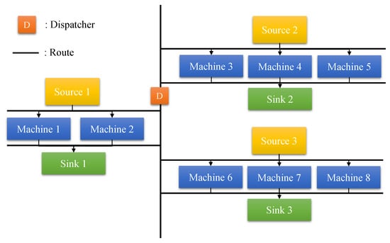
Figure 3.
Layout of the dynamic job-shop simulation environment.
4.2. Implementation Details
In this work, we proposed using the PPO algorithm as the default method for the DRL framework. The neural network with two hidden layers of 64 nodes and activation function can serve as the dispatcher, and the Adam optimizer is selected as the default optimizer for training the deep learning model. The parameters of PPO algorithm are shown in Table 2.
Table 2.
Parameter configuration of PPO algorithm.
In this work, we set up three scenarios for testing the proposed method and comparing it with other alternative methods. The setup parameters of the dynamic simulation environment are shown in Table 3. The changes are focused on the dispatcher speed factor and machine buffer factor. The mean time between failure (MTBF) and mean time off-line (MTOP) subject to exponential distribution which is defined as:
where is the expected value. The two parameters and of reward function are set to for the three scenarios shown in Table 3. Finally, the different combinations of and are tested to analyze their effect.
Table 3.
Experiment setup parameters.
4.3. Results and Analysis
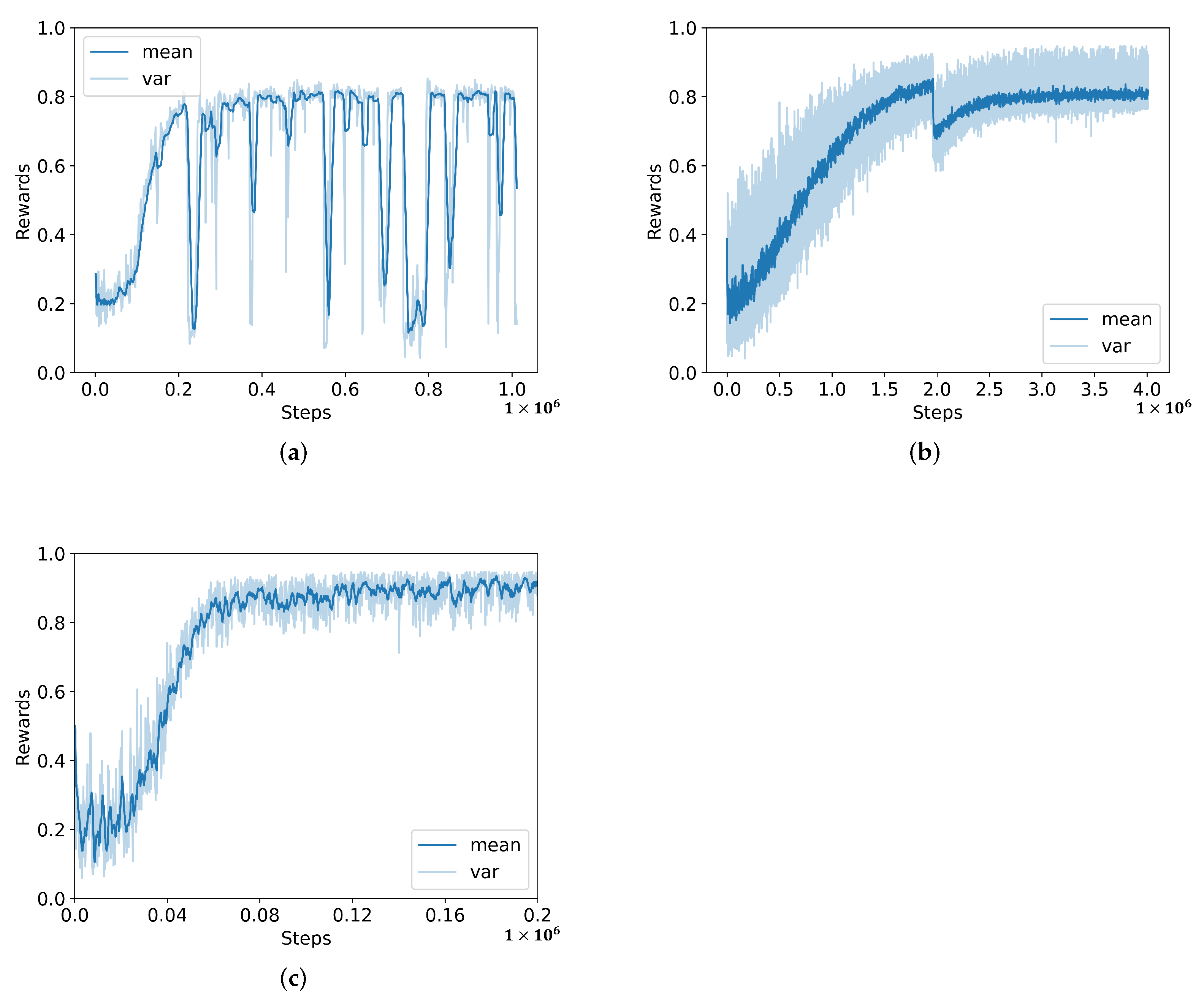
In order to testify the performance of the PPO algorithm [42], we compare it with two different methods including PG [44] and TRPO [45] under the default scenario. In this task, we select high dispatcher speed and very large machine buffer size so that the utilization of machines could be as high as possible. The overall learning process is shown in Figure 4. The results show that the DRL framework has the best performance by applying the PPO algorithm. It only takes simulation steps to converge, and the average rewards could be over . Meanwhile, the PG algorithm needs at least steps and the TRPO needs . All average rewards are under 0.85. Although the learning speed of PG is reasonable, the learning process of PG is seriously fluctuated. It is difficult to determine the optimal policy in this way. The TRPO algorithm has a stable learning process, however, it takes too many steps to determine the optimal solution. It is 20 times slower than the PPO algorithm.
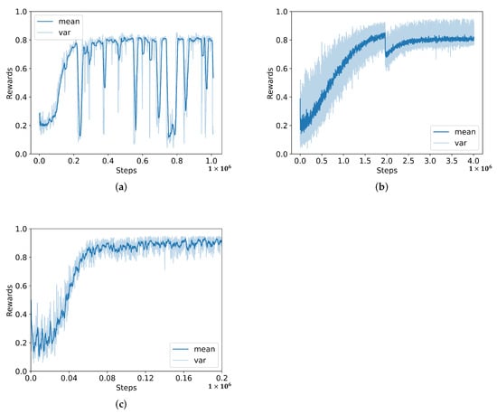
Figure 4.
Learning process of different algorithms; (a) policy gradient (PG), (b) trust region policy optimization (TRPO), and (c) proximal policy optimization (PPO).
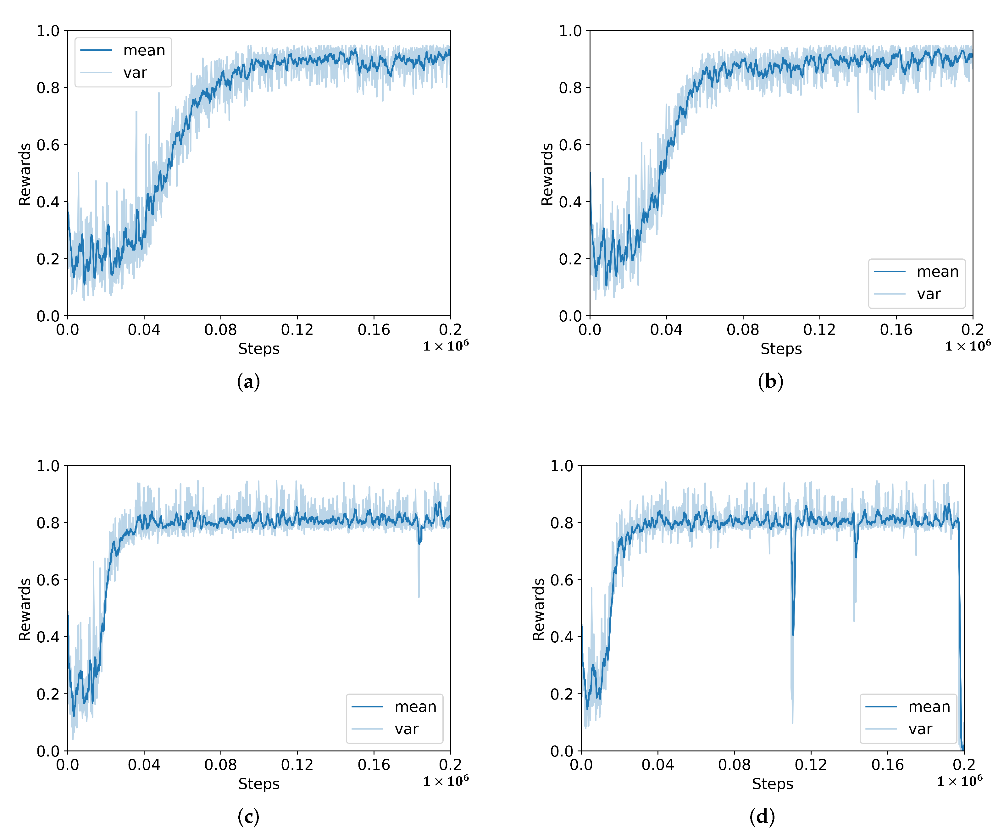
The parameters of the PPO algorithm are determined following the original research [42]. The clipping is the most sensitive parameter because it controls the range of policy progress for each update. As shown in Figure 5, the equal to obtains the best performance. The and results show they have a faster learning speed, but the average rewards could not reach the best average rewards. Meanwhile, the result shows that the best performance could be reached with longer learning steps.
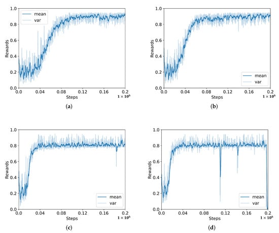
Figure 5.
Parameter sensitivity analysis of the PPO algorithm, (a) ; (b) ; (c) ; (d) .
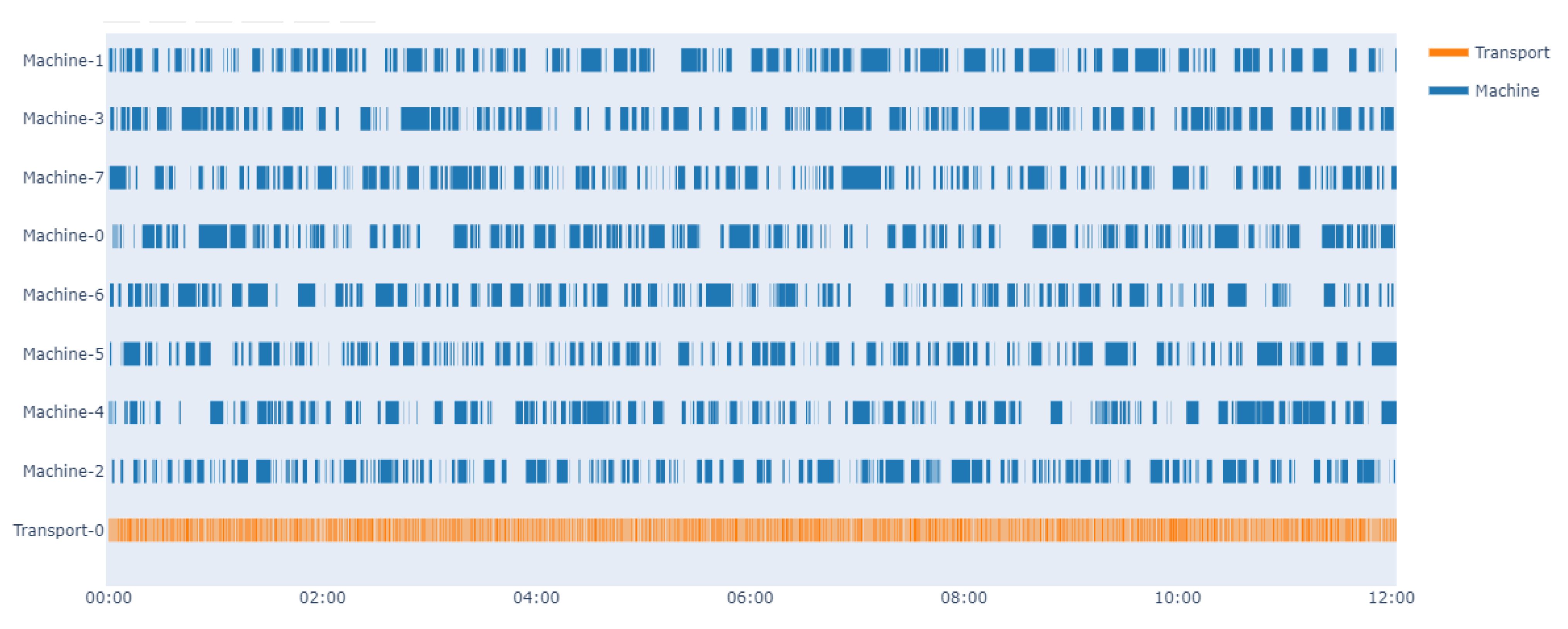
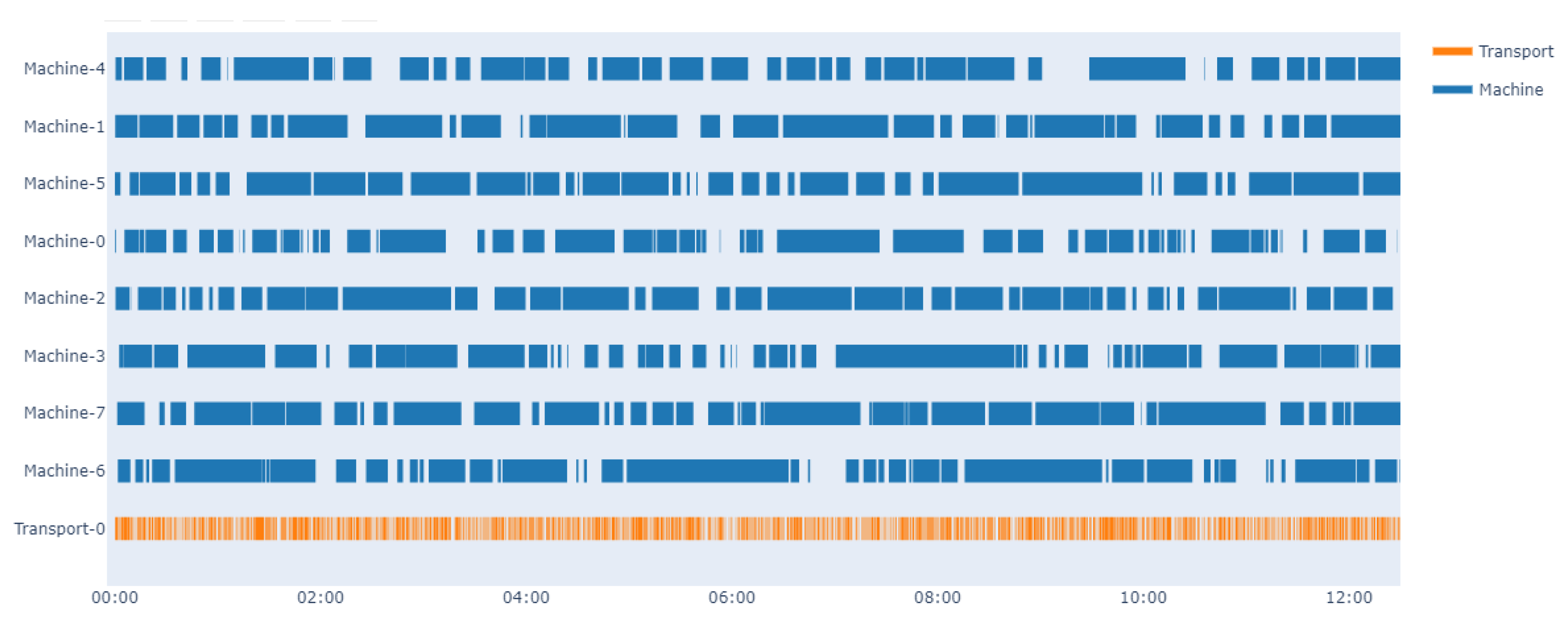
In order to demonstrate the performance and effectiveness of the proposed method, we test the optimal policy of the dispatcher under the same condition and compare it with a random policy. The Gantt chart of operation state is shown in Figure 6 and Figure 7. The dark blue represents the machines are working and the orange represents the dispatcher. The simulation environment is set to run 12 h with random policy and trained policy, respectively. Due to the existence of MTBF and MTOL, each machine breaks down, then needs a certain time period to recover. Therefore, one of the most important goals is to take full advantage of the machines when they become available. From the results, it is obvious that the learned policy could keep the machines continuously working, while it can be difficult to implement this goal with the random policy.
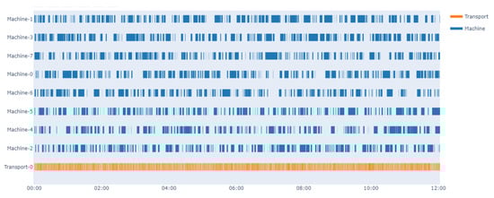
Figure 6.
Gantt chart of operating state working with random policy.
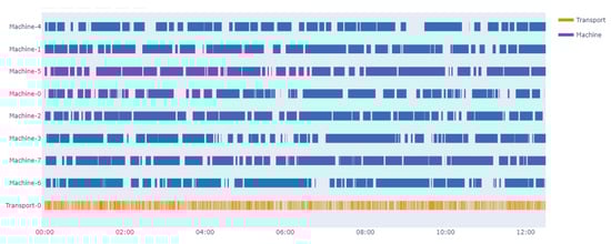
Figure 7.
Gantt chart of operating state working with optimal policy trained by the PPO algorithm.
To further analyze the proposed method, two scenarios have been set up for deploying quantitative comparison. In the first scenario, the dispatcher has a relatively slow speed () and the buffers of machines are relatively small (). On the contrary, the speed of the dispatcher is faster () and the machines have larger buffers (). Meanwhile, we compare these with different rule-based policies including Random, FIFO, and NJF [41]. Different reward functions are carried out for deep analysis. The average utilization of machines U, the average waiting time of orders (), and the alpha value () [46,47] are selected based on the evaluation criterion.
As shown in Table 4, the rule-based dispatching methods are compared with the random policy. Compared with random policy, both FIFO and NJF performed well. The NJF method is inclined to the utilization, while the FIFO method contributes more to waiting time. The utilization is affected by the transport speed of the dispatcher and the waiting time is affected by the size of the machine buffer. Therefore, compared with the first scenario, the U is higher and is fewer under the second scenario. The alpha value is a composite index combining multiple indicators, where a small value represents good performance.
Table 4.
Results for different rule-based heuristic dispatching approaches in both production scenarios.
According to the proposed DRL framework with the PPO algorithm, we test the performance in both production scenarios with different reward functions. In this experiment, we set two parameters and of all the reward functions as . The results are shown in Table 5. It is obvious that the performance of dispatchers under different reward functions reached a great level based on the comparison of results in Table 4. From the results, leads to a higher machine utilization and results in less order waiting time in both scenarios. The constant reward is also a good objective function but less flexible. The is to identify the optimal solution which can balance the utilization and waiting time. Just by adjusting different combinations of and , the dispatcher could learn different policies to meet the varying requirements. As shown in Table 6, the results show that utilization increase with the tend to , while the waiting time is controlled by . All in all, the results of different reward functions indicate that the proposed DRL framework can be more flexible than the general rule-based method. It could be implemented for different purposes by simply changing the reward shapes or their parameters. Meanwhile, the PPO algorithm guarantees the convergence efficiency of the optimal policy.
Table 5.
Results for PPO dispatching approaches under different reward function in both production scenarios.
Table 6.
Results for different combination of parameters and under reword function in production scenario 2.
5. Discussion and Conclusions
In this paper, we proposed a deep reinforcement learning framework with the PPO algorithm to address the dynamic scheduling problem of the job-shop manufacturing system. The new method is designed to improve learning efficiency and performance. The dynamic simulation of a real-world production environment was used for testifying the proposed method. The results demonstrate that the DRL with the PPO algorithm performs well, and it could obtain the fastest converge speed and the best rewards compared with the other state-of-the-art algorithms. The different reward functions on behalf of the multiple objectives were tested and compared with the rule-based heuristics approaches. The quantified results indicate that the proposed framework is more flexible and could perform effectively as well as the carefully designed rule-based method.
The proposed framework was testified and analyzed based on a real-world job-shop manufacturing system. However, there are other complicated industrial applications that need more comprehensive algorithms and solutions. Future extensions that may be beneficial to the proposed framework include the following:
- The optimal policy is only learned from the massive interaction data with the production environment. Expert knowledge would be considered as a support of further enhancement of efficiency and performance.
- In the current simulation, only one dispatcher is used as the transport agent. However, a dynamic simulation environment with multiple transport agents should be developed in future studies. The proposed deep reinforcement learning framework needs to be improved in multiagent situations.
- Toward the dynamic job-shop scheduling problem, other well-known algorithms, such as GA, PSO, and TLBO, will be implemented and compared with the deep reinforcement learning framework. With the corresponding benchmark problems developed, we will validate all the algorithms within the dynamic environment.
Author Contributions
Conceptualization, M.Z. and Y.X.; methodology, M.Z. and Y.L.; formal analysis, M.Z. and Y.L.; investigation, M.Z.; writing—original draft preparation, M.Z. and Y.H.; writing—review and editing, Y.L., N.A. and Y.X.; supervision, Y.X.; project administration, Y.X.; funding acquisition, Y.X. All authors have read and agreed to the published version of the manuscript.
Funding
This research was funded by RECLAIM project “Remanufacturing and Refurbishment Large Industrial Equipment” and received funding from the European Commission Horizon 2020 research and innovation programme under grant agreement No 869884.
Institutional Review Board Statement
Not applicable.
Informed Consent Statement
Not applicable.
Data Availability Statement
Data available in a publicly accessible repository that does not issue DOIs Publicly available datasets were analyzed in this study. This data can be found here: https://github.com/AndreasKuhnle/SimRLFab (accessed on 21 April 2022).
Conflicts of Interest
The authors declare no conflict of interest.
References
- Sanchez, M.; Exposito, E.; Aguilar, J. Autonomic computing in manufacturing process coordination in industry 4.0 context. J. Ind. Inf. Integr. 2020, 19, 100159. [Google Scholar] [CrossRef]
- Csalódi, R.; Süle, Z.; Jaskó, S.; Holczinger, T.; Abonyi, J. Industry 4.0-driven development of optimization algorithms: A systematic overview. Complexity 2021, 2021, 6621235. [Google Scholar] [CrossRef]
- Zenisek, J.; Wild, N.; Wolfartsberger, J. Investigating the potential of smart manufacturing technologies. Procedia Comput. Sci. 2021, 180, 507–516. [Google Scholar] [CrossRef]
- Popov, V.V.; Kudryavtseva, E.V.; Kumar Katiyar, N.; Shishkin, A.; Stepanov, S.I.; Goel, S. Industry 4.0 and Digitalisation in Healthcare. Materials 2022, 15, 2140. [Google Scholar] [CrossRef]
- Zhang, W.; Yang, D.; Wang, H. Data-driven methods for predictive maintenance of industrial equipment: A survey. IEEE Syst. J. 2019, 13, 2213–2227. [Google Scholar] [CrossRef]
- Kleindorfer, P.R.; Singhal, K.; Van Wassenhove, L.N. Sustainable operations management. Prod. Oper. Manag. 2005, 14, 482–492. [Google Scholar] [CrossRef]
- Kiel, D.; Müller, J.M.; Arnold, C.; Voigt, K.I. Sustainable industrial value creation: Benefits and challenges of industry 4.0. In Digital Disruptive Innovation; World Scientific: Singapore, 2020; pp. 231–270. [Google Scholar]
- Saxena, P.; Stavropoulos, P.; Kechagias, J.; Salonitis, K. Sustainability assessment for manufacturing operations. Energies 2020, 13, 2730. [Google Scholar] [CrossRef]
- Henao, R.; Sarache, W.; Gómez, I. Lean manufacturing and sustainable performance: Trends and future challenges. J. Clean. Prod. 2019, 208, 99–116. [Google Scholar] [CrossRef]
- Rajeev, A.; Pati, R.K.; Padhi, S.S.; Govindan, K. Evolution of sustainability in supply chain management: A literature review. J. Clean. Prod. 2017, 162, 299–314. [Google Scholar] [CrossRef]
- Serrano-Ruiz, J.C.; Mula, J.; Poler, R. Smart manufacturing scheduling: A literature review. J. Manuf. Syst. 2021, 61, 265–287. [Google Scholar] [CrossRef]
- Serrano-Ruiz, J.C.; Mula, J.; Poler, R. Development of a multidimensional conceptual model for job shop smart manufacturing scheduling from the Industry 4.0 perspective. J. Manuf. Syst. 2022, 63, 185–202. [Google Scholar] [CrossRef]
- Zhang, X.; Liu, W. Complex equipment remanufacturing schedule management based on multi-layer graphic evaluation and review technique network and critical chain method. IEEE Access 2020, 8, 108972–108987. [Google Scholar] [CrossRef]
- Yu, J.M.; Lee, D.H. Scheduling algorithms for job-shop-type remanufacturing systems with component matching requirement. Comput. Ind. Eng. 2018, 120, 266–278. [Google Scholar] [CrossRef]
- Cai, L.; Li, W.; Luo, Y.; He, L. Real-time scheduling simulation optimisation of job shop in a production-logistics collaborative environment. Int. J. Prod. Res. 2022, 1–21. [Google Scholar] [CrossRef]
- Satyro, W.C.; de Mesquita Spinola, M.; de Almeida, C.M.; Giannetti, B.F.; Sacomano, J.B.; Contador, J.C.; Contador, J.L. Sustainable industries: Production planning and control as an ally to implement strategy. J. Clean. Prod. 2021, 281, 124781. [Google Scholar] [CrossRef]
- Wang, L.; Hu, X.; Wang, Y.; Xu, S.; Ma, S.; Yang, K.; Liu, Z.; Wang, W. Dynamic job-shop scheduling in smart manufacturing using deep reinforcement learning. Comput. Netw. 2021, 190, 107969. [Google Scholar] [CrossRef]
- Garey, M.R.; Johnson, D.S.; Sethi, R. The complexity of flowshop and jobshop scheduling. Math. Oper. Res. 1976, 1, 117–129. [Google Scholar] [CrossRef]
- Manne, A.S. On the job-shop scheduling problem. Oper. Res. 1960, 8, 219–223. [Google Scholar] [CrossRef] [Green Version]
- Van Laarhoven, P.J.; Aarts, E.H.; Lenstra, J.K. Job shop scheduling by simulated annealing. Oper. Res. 1992, 40, 113–125. [Google Scholar] [CrossRef] [Green Version]
- Wang, Y.; Qing-dao-er-ji, R. A new hybrid genetic algorithm for job shop scheduling problem. Comput. Oper. Res. 2012, 39, 2291–2299. [Google Scholar]
- Sha, D.; Lin, H.H. A multi-objective PSO for job-shop scheduling problems. Expert Syst. Appl. 2010, 37, 1065–1070. [Google Scholar] [CrossRef]
- Xu, Y.; Wang, L.; Wang, S.y.; Liu, M. An effective teaching–learning-based optimization algorithm for the flexible job-shop scheduling problem with fuzzy processing time. Neurocomputing 2015, 148, 260–268. [Google Scholar] [CrossRef]
- Du, Y.; Li, J.q.; Chen, X.l.; Duan, P.y.; Pan, Q.k. Knowledge-Based Reinforcement Learning and Estimation of Distribution Algorithm for Flexible Job Shop Scheduling Problem. IEEE Trans. Emerg. Top. Comput. Intell. 2022, 1–15. [Google Scholar] [CrossRef]
- Mohan, J.; Lanka, K.; Rao, A.N. A review of dynamic job shop scheduling techniques. Procedia Manuf. 2019, 30, 34–39. [Google Scholar] [CrossRef]
- Azadeh, A.; Negahban, A.; Moghaddam, M. A hybrid computer simulation-artificial neural network algorithm for optimisation of dispatching rule selection in stochastic job shop scheduling problems. Int. J. Prod. Res. 2012, 50, 551–566. [Google Scholar] [CrossRef]
- Wang, C.; Jiang, P. Manifold learning based rescheduling decision mechanism for recessive disturbances in RFID-driven job shops. J. Intell. Manuf. 2018, 29, 1485–1500. [Google Scholar] [CrossRef]
- Zhao, Y.; Zhang, H. Application of machine learning and rule scheduling in a job-shop production control system. Int. J. Simul. Model 2021, 20, 410–421. [Google Scholar] [CrossRef]
- Tian, W.; Zhang, H. A dynamic job-shop scheduling model based on deep learning. Adv. Prod. Eng. Manag. 2021, 16, 23–36. [Google Scholar] [CrossRef]
- Tassel, P.; Gebser, M.; Schekotihin, K. A reinforcement learning environment for job-shop scheduling. arXiv 2021, arXiv:2104.03760. [Google Scholar]
- Kuhnle, A.; Schäfer, L.; Stricker, N.; Lanza, G. Design, implementation and evaluation of reinforcement learning for an adaptive order dispatching in job shop manufacturing systems. Procedia CIRP 2019, 81, 234–239. [Google Scholar] [CrossRef]
- Kuhnle, A.; Röhrig, N.; Lanza, G. Autonomous order dispatching in the semiconductor industry using reinforcement learning. Procedia CIRP 2019, 79, 391–396. [Google Scholar] [CrossRef]
- Xia, K.; Sacco, C.; Kirkpatrick, M.; Saidy, C.; Nguyen, L.; Kircaliali, A.; Harik, R. A digital twin to train deep reinforcement learning agent for smart manufacturing plants: Environment, interfaces and intelligence. J. Manuf. Syst. 2021, 58, 210–230. [Google Scholar] [CrossRef]
- Kuhnle, A.; Kaiser, J.P.; Theiß, F.; Stricker, N.; Lanza, G. Designing an adaptive production control system using reinforcement learning. J. Intell. Manuf. 2021, 32, 855–876. [Google Scholar] [CrossRef]
- Zhao, Y.; Wang, Y.; Tan, Y.; Zhang, J.; Yu, H. Dynamic Jobshop Scheduling Algorithm Based on Deep Q Network. IEEE Access 2021, 9, 122995–123011. [Google Scholar] [CrossRef]
- Wang, H.; Sarker, B.R.; Li, J.; Li, J. Adaptive scheduling for assembly job shop with uncertain assembly times based on dual Q-learning. Int. J. Prod. Res. 2021, 59, 5867–5883. [Google Scholar] [CrossRef]
- Zeng, Y.; Liao, Z.; Dai, Y.; Wang, R.; Li, X.; Yuan, B. Hybrid intelligence for dynamic job-shop scheduling with deep reinforcement learning and attention mechanism. arXiv 2022, arXiv:2201.00548. [Google Scholar]
- Luo, S.; Zhang, L.; Fan, Y. Dynamic multi-objective scheduling for flexible job shop by deep reinforcement learning. Comput. Ind. Eng. 2021, 159, 107489. [Google Scholar] [CrossRef]
- Kaelbling, L.P.; Littman, M.L.; Moore, A.W. Reinforcement learning: A survey. J. Artif. Intell. Res. 1996, 4, 237–285. [Google Scholar] [CrossRef] [Green Version]
- Schulman, J.; Moritz, P.; Levine, S.; Jordan, M.; Abbeel, P. High-dimensional continuous control using generalized advantage estimation. arXiv 2015, arXiv:1506.02438. [Google Scholar]
- Waschneck, B.; Altenmüller, T.; Bauernhansl, T.; Kyek, A. Production Scheduling in Complex Job Shops from an Industry 4.0 Perspective: A Review and Challenges in the Semiconductor Industry. In Proceedings of the SAMI@ iKNOW, Graz, Austria, 19 October 2016; pp. 1–12. [Google Scholar]
- Schulman, J.; Wolski, F.; Dhariwal, P.; Radford, A.; Klimov, O. Proximal policy optimization algorithms. arXiv 2017, arXiv:1707.06347. [Google Scholar]
- Mönch, L.; Fowler, J.W.; Mason, S.J. Production Planning and Control for Semiconductor Wafer Fabrication Facilities: Modeling, Analysis, and Systems; Springer Science & Business Media: Berlin, Germany, 2012; Volume 52. [Google Scholar]
- Silver, D.; Lever, G.; Heess, N.; Degris, T.; Wierstra, D.; Riedmiller, M. Deterministic policy gradient algorithms. In Proceedings of the International Conference on Machine Learning, PMLR, Beijing, China, 21–26 June 2014; pp. 387–395. [Google Scholar]
- Schulman, J.; Levine, S.; Abbeel, P.; Jordan, M.; Moritz, P. Trust region policy optimization. In Proceedings of the International Conference on Machine Learning, PMLR, Lille, France, 6–11 July 2015; pp. 1889–1897. [Google Scholar]
- Boebel, F.; Ruelle, O. Cycle time reduction program at ACL. In Proceedings of the IEEE/SEMI 1996 Advanced Semiconductor Manufacturing Conference and Workshop. Theme-Innovative Approaches to Growth in the Semiconductor Industry. ASMC 96 Proceedings, Cambridge, MA, USA, 12–14 November 1996; pp. 165–168. [Google Scholar]
- Schoemig, A.K. On the corrupting influence of variability in semiconductor manufacturing. In Proceedings of the 31st Conference on Winter Simulation: Simulation—A Bridge to the Future, Phoenix, AZ, USA, 5–8 December 1999; Volume 1, pp. 837–842. [Google Scholar]

Publisher’s Note: MDPI stays neutral with regard to jurisdictional claims in published maps and institutional affiliations. |
© 2022 by the authors. Licensee MDPI, Basel, Switzerland. This article is an open access article distributed under the terms and conditions of the Creative Commons Attribution (CC BY) license (https://creativecommons.org/licenses/by/4.0/).