Abstract
Capacity curves obtained from nonlinear static analyses are widely used to perform seismic assessments of structures as an alternative to dynamic analysis. This paper presents a novel ‘en masse’ method to assess the seismic vulnerability of urban areas swiftly and with the accuracy of mechanical methods. At the core of this methodology is the calculation of the capacity curves of low-rise reinforced concrete buildings using neural networks, where no modeling of the building is required. The curves are predicted with minimal error, needing only basic geometric and material parameters of the structures to be specified. As a first implementation, a typology of prismatic buildings is defined and a training set of more than 7000 structures generated. The capacity curves are calculated through push-over analysis using SAP2000. The results feature the prediction of 100-point curves in a single run of the network while maintaining a very low mean absolute error. This paper proposes a method that improves current seismic assessment tools by providing a fast and accurate calculation of the vulnerability of large sets of buildings in urban environments.
1. Introduction
The objective of this research is to develop an accurate technique to perform ‘en masse’ seismic assessments of low-rise buildings by predicting capacity curves with machine learning (ML), employing a simple set of the buildings’ geometrical parameters, rather than engaging with a tedious modeling process.
There are numerous studies focused on the seismic risk and vulnerability of buildings, based on analyzing the risk on either an urban or a building scale. Urban-scale analyses are mainly based on macro-seismic approaches [1,2]. Because of the obvious difficulty of modeling each building individually (the mechanical approach), these methods are characterized by a trade-off between accuracy and effectiveness in terms of time and resources. Typically, their rationales boil down to the assessment of urban areas by grouping similar buildings into typologies or building classes of which the seismic behavior has been previously calculated in depth [3,4,5]. For example, in Europe, it is common to use the building classes of the RISK-UE project [6]. This methodology was applied to the city of Barcelona [7] and to some Portuguese cities [8]. Hybrid approaches can, however, improve the accuracy of macro-seismic assessments by combining the latter method with other techniques. For instance, visual screening can improve the knowledge level of the structures under assessment, which in turn helps to create more representative building classes and increase accuracy. Other hybrid approaches include identifying and modeling those features of the structures that have a greater impact in their seismic performance by means of sensitivity or parametric analyses [9,10]. Empirical methods have also been used to perform seismic assessments on an urban scale [11]. This approach relies heavily on damage data from previous earthquakes and their impact on the building stock, which are not always easy to obtain.
In contrast to the above approaches, when studying a building in detail, a specific mechanical model for the building is defined and calculated. This is much more accurate, but requires many hours of work: the blueprints of the building must be obtained or drafted, the parameters of the materials must be determined, a model must be built by a specialist and, finally, the results are obtained. This is obviously excessively time-consuming when calculating a large number of buildings. However, by shortcutting the modeling process with ML, the methodology presented in this paper begets the advantages from both worlds (mechanical and macro-seismic) while having none of their drawbacks. In short, the main innovation and impact of this paper is that it sets out a methodology for an ‘en masse’ mechanical approach that is set to replace macro-seismic methods for the seismic assessment of urban areas and real-time evaluation tools.
The seismic behavior of individual structures can be assessed by means of dynamic or static analyses, accounting for their nonlinear modeling. Dynamic analyses require higher computational burdens than static ones. Contrariwise, static analyses are characterized by an affordable computational time while retaining high performance targets. In this work, nonlinear static analyses are performed to assess the seismic behavior of the structures following Eurocode 8, commonly known as push-over. This method is based on the calculation of the capacity curves of the building, which capture the relationship between basal shear and roof displacement under an incremental force applied to the structure. Nonlinear static has been selected over dynamic analysis mainly because (i) low-rise and mainly regular buildings are assessed, for which push-over analyses produce reliable results [12,13]. In the case of mid- and high-rise buildings, dynamic analyses would be required. Hence, dynamic analyses like time history analysis are usually carried out as in [14]. (ii) The time history analysis method requires real accelerograms to determine the behavior of the structure for a specific seismic record. This is a well-known dynamic approach. However, this is not a generic method, as the aim of this research requires. It should be noted that this method is mainly used to perform exhaustive analyses of particular case study buildings or infrastructures such as tunnels [15], slopes [16] or special structures [17]. (iii) The goal of this work is to develop a general method that can allow the determination of a capacity curve for all types of regular low-rise RC structures in a fast and simple manner. The choice of push-over over time history analysis has facilitated the generation of a dataset large enough to achieve this last objective.
As a first implementation of the proposed method, a typology of low-rise prismatic reinforced concrete (RC) buildings is defined and a training set of more than 7000 structures is parametrically generated. The capacity curves of these models are obtained by means of push-over analysis using SAP2000 software. After defining and training an appropriate neural network model, full capacity curves are predicted in a single run of the network, with a resolution of up to 100 points. This benchmark is substantially higher than previous research that employed less efficient and comprehensive approaches, e.g., one point at a time. The problem with this common approach is not only that it is slower, more tedious and complicated, but also that the information of where the curve ends is completely lost.
However, push-over analysis is still time-consuming, computationally expensive and requires advanced modeling expertise. In general, the 3D modeling of structures within engineering software packages is not an option when one needs to assess a large number of buildings. For this reason, there is an increasing volume of research that advocates the use of ML techniques that enable bypassing these limitations. One such method that has gained interest in recent years is artificial neural networks (ANN), mainly due to the extraordinary capability of these networks to approximate very complex functions. ANN can perform nonlinear modeling without prior knowledge of the relationships between the input and output variables. Consequently, they constitute a general and flexible modeling tool for prediction. It comes as no surprise that many engineering disciplines are witnessing an intense engagement with neural network models to solve a broad range of challenging problems [18,19,20,21,22,23,24,25].
The choice of ANN responds, on the one hand, to the fact that these models are naturally well suited for the challenges outlined above (strong nonlinearity and a large regression output of up to 100 points). On the other hand, it may be noted that the finite element method (FEM), as used in the SAP2000 calculations of this study, aims to solve differential functions that arise from structural analysis. Neural networks, in turn, are naturally equipped to deal with continuous and differentiable data that allow for an error optimization process through the gradient descent algorithm. In other words, the differentiable character of the data generated by FEM calculations is another aspect that makes the problem under study in this paper a good fit for a neural network model.
Many studies exist that use ML methods to assess the damage, vulnerability and response of buildings under seismic action, ranging from entire structures to structural elements and material stress-tests. In [26], a very similar approach to the method proposed in this paper is conducted to assess a set of 30 buildings using time history analysis. The present research expands the latter study to account for a much broader range of buildings based on a training set of more than 7000 parametrically generated structures. Similarly, a very in-depth application of neural networks was carried out in [24] to predict seismic-induced stress in specific elements of a two-span and two-story structure. In contrast with the present research, their model is specific to a case study structure, and the trained networks cannot be used to predict stresses in similar yet different structures. This is also the case in [27], where a recurrent neural network model with Bayesian training and mutual information is used for the response prediction of large buildings. Recurrent nets are a common choice for time series and, more broadly, data that feature temporal correlations. Although not specific to response prediction, other work featuring recurrent models in the area of seismic analysis can also be found in the literature [28,29]. In light of the results obtained with the methodology presented in the present paper, the authors are of the opinion that the feedforward model chosen in this work was sufficient to address the problem at hand. However, a recurrent approach would perhaps be better suited for the challenges described in the Future Work section (for instance, extending the proposed methodology to high-rise buildings). Additionally, a good number of recent studies have focused on several improvements of the ML algorithms and methodologies used to assess the impact of seismic actions on structures [30,31,32,33,34,35].
ANN were also used in a classification fashion to establish which damage-level category a certain structure would fall into for a given seismic demand [36]. Therefore, their approach was to use neural networks for pattern recognition based on structural parameters. In the method proposed here, a multidimensional regression approach to the application of neural networks is used to predict capacity curves, which provide a more detailed behavior of the structural damage. In the case of [37], a very similar approach to the present work was adopted to predict fragility curves with neural networks and other ML methods. Yet, since their study was based on dynamic analysis, capacity curves were not considered, as opposed to the static approach employed in this paper. Furthermore, fragility curves were not computed in a single run of the network, as the present method proposes. Instead, each run estimates an individual pair of coordinates, and then the curves are rebuilt based on these estimations.
Other data mining techniques including ANN were employed to predict the performance point of school buildings under seismic action [37]. Similarly, in [38], the same objective was targeted using a genetic algorithm instead, achieving similar levels of error. The advantage of this last approach is that their model provides a transparent mathematical formula for the prediction of the performance point. However, both studies focus on predicting the performance point directly without considering the capacity curves of the buildings. This imposes many levels of complexity on the model, thus reducing the accuracy.
Other work used neural networks to make use of simplified approaches to determine the seismic performance of buildings. In [39], an experimental database was employed to train a neural network with very few input parameters, seven in total, in order to predict stress and deformation values at specific locations within masonry-infilled RC frames under seismic action. The study aims to simplify the complex modeling of mixed-element structures, but is still limited in the scope of application due to a much-reduced number of input parameters. Finally, in [40], neural networks were used to predict a bilinear simplification of capacity curves with accurate results. By contrast, in the methodology proposed in this paper, original capacity curves are predicted without simplification, broadening their scope of application.
As a summary, the main contribution of this work with regard to previous research is centered on the model’s ability to instantly perform a mechanical seismic assessment of an uncountable number of diverse buildings beyond the already vast training dataset. Additionally, this study delivers an important contribution by presenting a unified methodology that allows for the prediction of capacity curves (i) using simple input parameters derived from the geometric and material properties of the buildings alone, (ii) performing in a plastic regime (iii) in high resolution of up to 100 points per curve, (iv) in a single and coherent process (rather than in a point-by-point fashion), (v) for entire buildings with a great range of variability in size (limited to prismatic low-rise) and (vi) with immediate applicability to real-world emergency relief use cases under the seismic regulations in Eurocode 8.
2. Methodology
2.1. Parametric Generation of Structures
In order to automate the generation of a training set for the neural network, the first step is to generate a large number of virtual structures, all different from each other, but falling under a typology that is representative of the buildings in many urban areas of the Algarve–Huelva region. To carry out this task, a set of parameters and value ranges was chosen based on the list of buildings elaborated for the area of study. These parameters and their value ranges are defined in Table 1. The choice of features used for the parameterization responds to the need for (i) finding a set or vector large enough to provide a meaningful characterization of the buildings, while (ii) selecting features that are easily obtainable from local governmental databases without the need to engage in building surveys on the ground. The ranges and steps specified for the values of the parameters were adjusted to empirical observations from the aforementioned databases, as well as local advice from industry experts in the region of study.

Table 1.
Parameters for random generation of structures.
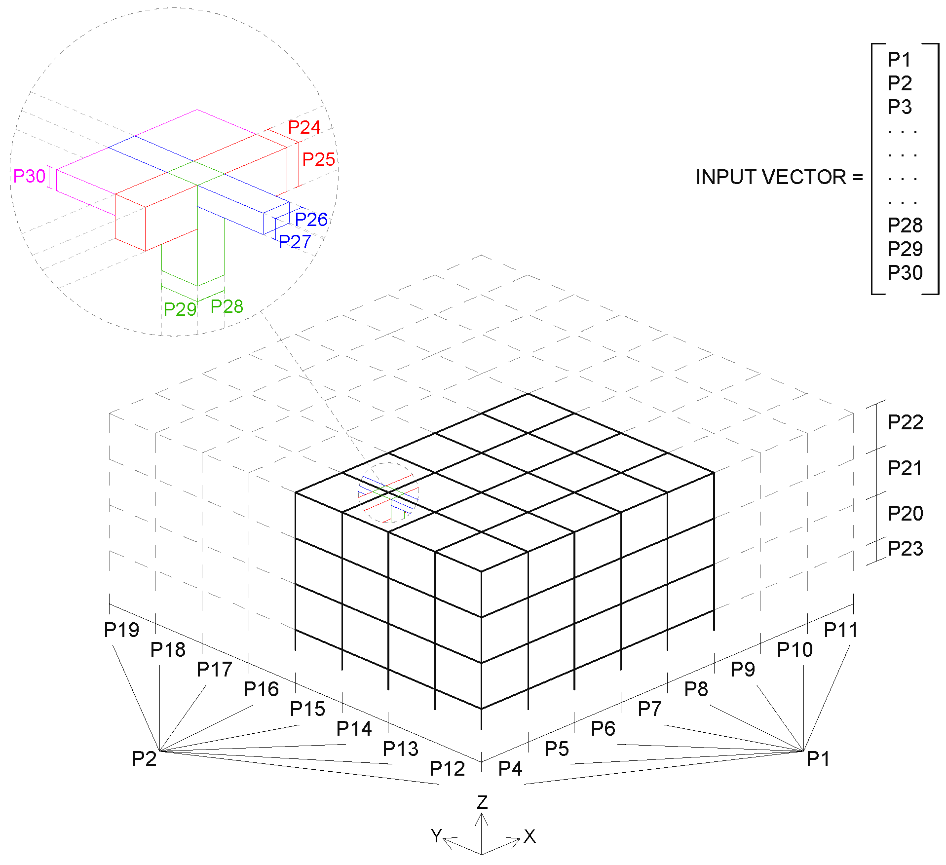
For every structure, all slabs share the same height and the same goes for the beams. The dimensions of the beams (both load-bearing and non-load-bearing) are calculated according to their span, and then a single pair of values (width, height) is fixed for each given structure, which will be the most restrictive (largest). Supports are always 30 × 30 across all structures and load-bearing frames are aligned to the X axis. A diagram illustrating all of the parameters that make up the input vector for the network is shown in Figure 1.
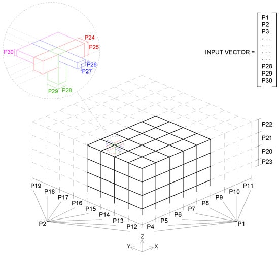
Figure 1.
Diagram of the structure’s geometric parameters that are used as network inputs.
Looking at the geometric variations in terms of the number of spans in X, Y, Z and the dimensions of each of them, the total number of different structures that result from all possible combinations of these parameters, with the given value ranges and value steps, is:
where T = the total amount of unique structures possible, nx, ny, nz = the number of spans in X, Y and Z, respectively, and sx, sy, sz = the number of steps in X, Y and Z, respectively. According to this formula, T = 9 × 9 × 3 × 249 × 249 × 103 and therefore, T > 1018.
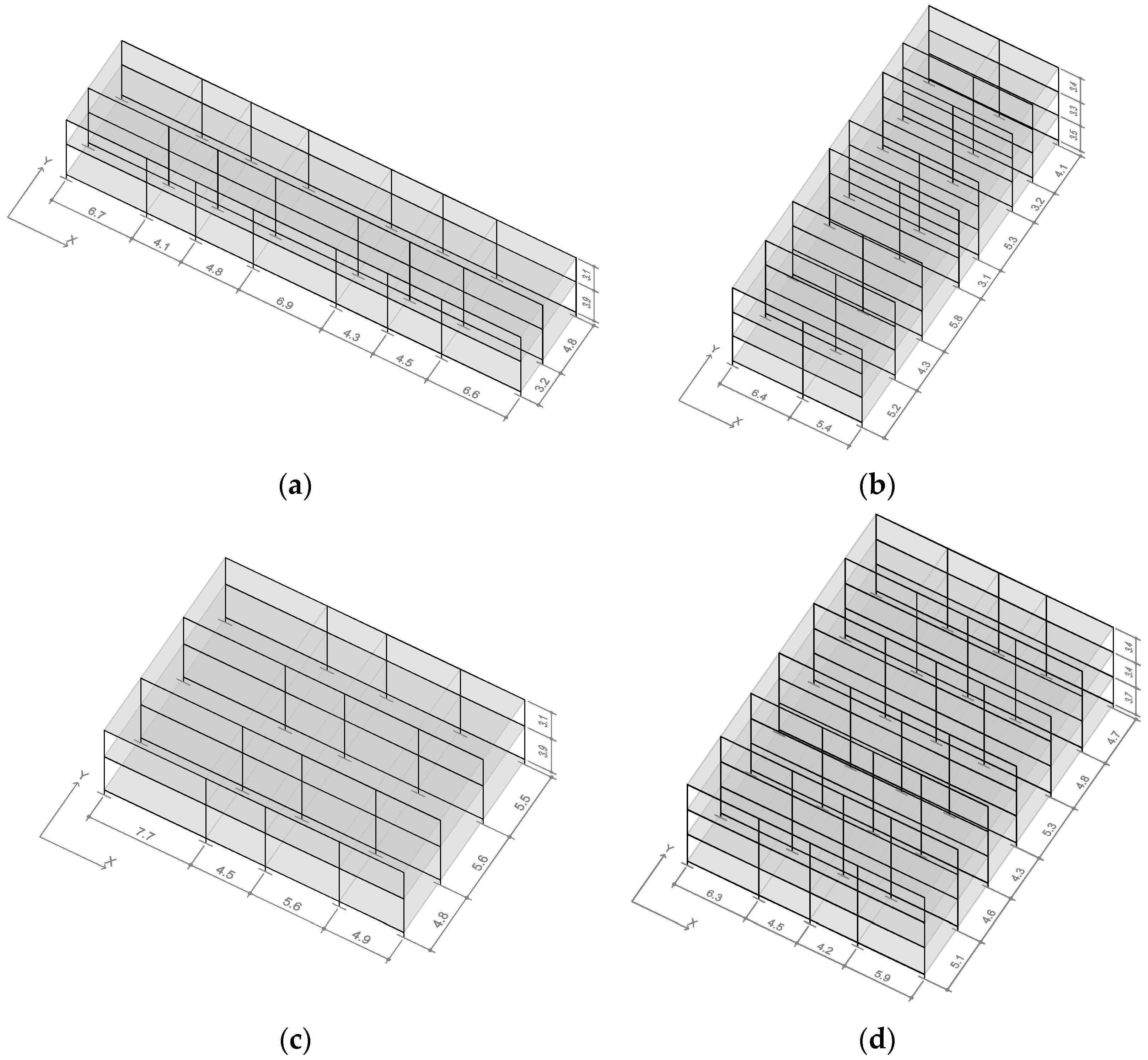
For the training set, more than 7000 unique structures are generated. Since there are more than 1018 possibilities, these are created using random values within the given ranges. In some studies, certain combinations of parameters have been filtered out to avoid computing structures that are not represented in a given database [41]. However, in this work, all possible combinations are computed. While this might be less effective computationally, it allows the model to be more general or inclusive, provided that the results are still satisfactory. Figure 2 shows a visualization of some of the generated structures.
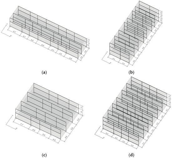
Figure 2.
Randomly generated structures. (a) Sample #1355, (b) sample #147, (c) sample #1926 and (d) sample #639. For each structure, a vector containing the 30 values that result from applying the above parameters is stored and will be used as the input of the neural network (after normalization).
2.2. Push-Over Analysis
Push-over analysis methods for seismic calculation have been extensively developed and compared to full dynamic analysis. Such studies [13] establish a firm resolution on the applicability of push-over methods for estimating the strength capacity in a post-elastic range, especially for regular low-rise buildings which is the scope of the present work. In this method, the progress of the overall capacity curves of the structure is traced by measuring the basal shear values versus their corresponding displacements.
Obtaining capacity curves requires an analysis that considers the plastic state of the RC structure. The non-linear analysis of RC structures is a very complex task, which usually requires finite element analysis as a base. However, there is a simplified method to calculate nonlinear behavior in RC structures, which simulates plastic deformation in RC elements by introducing plastic hinges in appropriate locations within these elements [42]. In this methodology, all of the plastic behavior of the structure is reduced to these specific points, facilitating faster and easier modeling and calculation. This simplification is contemplated in the ASCE-41-13 [43] and has been proved satisfactory for the seismic assessment of low-rise buildings [44].
The capacity curves of all of the structures in the training set were calculated in SAP2000 via the Open API in the X direction using the following scheme:
- -
- All supports are rigidly clamped to their foundation.
- -
- Slabs are computed as horizontal diaphragms, as in [45].
- -
- The values of structural materials, including the mechanical properties of concrete, are obtained from the Spanish Technical Code of Buildings (CTE) [46] and the Spanish Reinforced Concrete Code (EHE-08) [47] at the time of construction.
- -
- Reinforcements of RC elements are defined according to the Spanish Reinforced Concrete Code (EHE) [47], as presented in Table 2.
Table 2. Rebar reinforcement scheme.
- -
- As recommended in [44], the nonlinear behavior of RC elements is simulated by defining plastic hinges within them, according to the ASCE-41-13. In a similar way to [44,48], PM2M3 plastic hinges are introduced in the columns, while the M3 type is used in the beams. They are introduced at the ends of the beams and the columns, as in [49] and as recommended in Eurocode 8 (EC-8) [50].
- -
- The capacity curves are not truncated by shear or flexural failure and, therefore, remain in the ductile domain at all times.
- -
- The contribution of the infill walls is not considered, as in [51].
- -
- Gravitational loads (G) are also obtained from the buildings’ data and the CTE. These are combined according to the seismic combinations and coefficients established in the Spanish seismic code (NCSE-02) [46], as shown in Equation (2).where W is the weight of the structural elements, i.e., the RC beams and columns. D represents the design dead loads, i.e., the weight of the RC ribbed slabs (3.0 kPa), internal partitions (1 kPa), ceiling (0.5 kPa), ceramic flooring (1 kPa) and infills (10 kN/m) and Q is the live load for public spaces (3 kPa).
- -
- Push-over loads are applied to all nodes in the XZ/YZ plane proportional to the loaded slab weight and are determined by the following formula:where FL is the total amount of horizontal force applied to each level, ZL is the height in meters from the ground to the slab where the load is being applied, and Gs is the combination of the structural weight, dead loads and live load of the slab, as described above. Note that although EC-8 obliges calculating two load patterns (the other is a load pattern proportional to the first mode of vibration of the building), in [13], it was demonstrated that for prismatic low-rise structures, there are no substantial differences between the two.
- -
- The control point for displacements is located at the highest, most central point of the structure.
The push-over calculations in this work are performed exclusively in one direction. To obtain the curve in the other direction (Y), it suffices to input the geometric parameters of the building in the neural network, as viewed from that axis.
Once the calculation was done in SAP2000 using all of the above specifications, the capacity curves obtained via the Open API for each randomly generated structure were stored for training and validation. In order to ensure that the results obtained were consistent with manual modeling, a series of structures were tested both manually and through the automated procedure, yielding the same results.
From all of the curves stored, 70% were randomly selected and used as the expected output for the training process of the neural network (training dataset). The remaining 30% were used as a validation dataset to evaluate the accuracy of the network in predicting the coordinates of the capacity curves that had not taken part in the training process. Additionally, the random split between training and validation was performed a total of 60 times to ensure that the results were not affected by the distribution of samples. The final results in this paper show average, minimum and maximum values corresponding to this set of randomized splits. Figure 3 shows a selection of these curves.
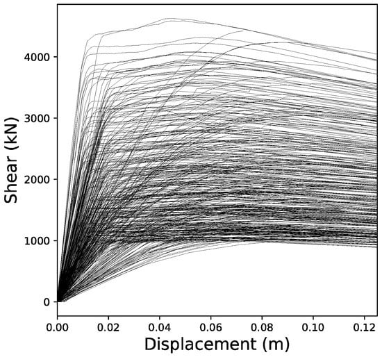
Figure 3.
Capacity curves from a selection of over 7000 randomly generated buildings.
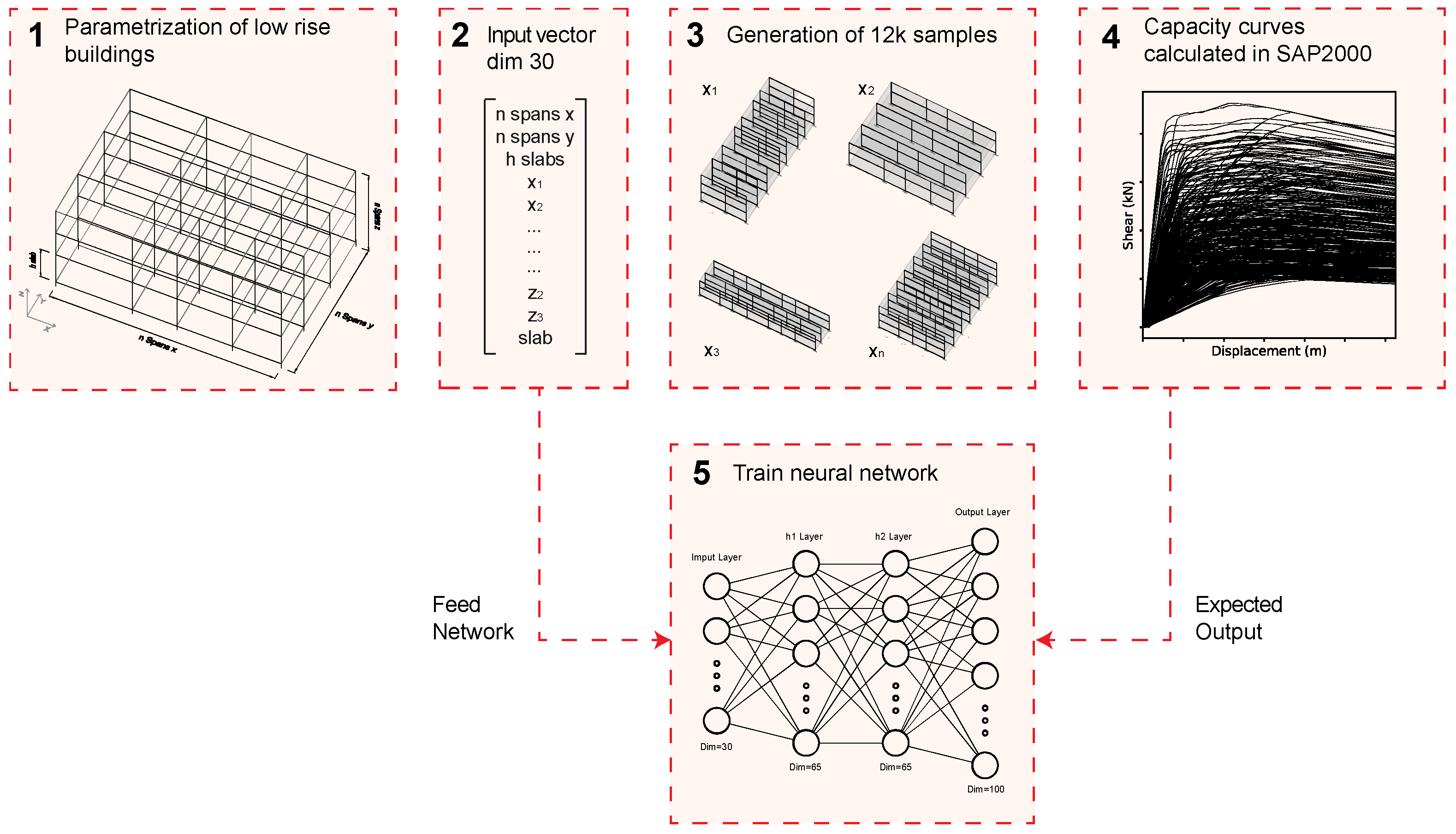
The methodology presented here predicts the full original capacity curve. When carrying out a push-over analysis with SAP2000, the stopping of the capacity curve may respond to three different causes: (i) a roof displacement at the control point is reached that is sufficient to cause a 20% drop from peak shear (following the guidelines of Eurocode 8 in section C.3.3); (ii) a local mechanism is formed; or (iii) a problem or lack of convergence is found in the analysis. Unfortunately, there is no way of concluding which motive has caused the ending of the process by exclusively analyzing the resulting curve. In this sense, the prediction of that last point of the curve will not be very accurate because the ANN is trying to predict a value that is not entirely related to the physical properties of the structure. Nevertheless, this ability of the method will become meaningful in future study, in which a physically representative collapse criterion (i.e., limiting the rotation of the plastic hinges in concrete buildings) could be implemented in order to establish the end point of the original curves. A graphic overview of the main concept behind the method proposed is shown in Figure 4.
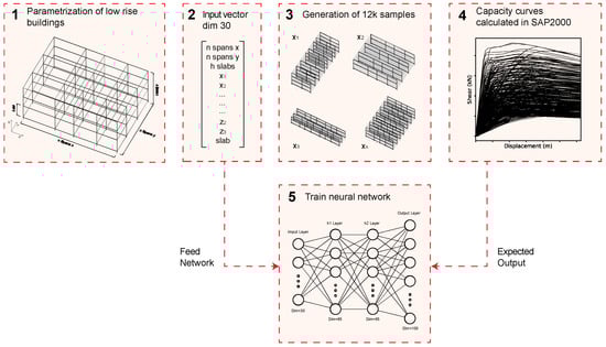
Figure 4.
Diagram of methodology proposed for the training of the network.
2.3. Curve Data Processing
Some studies, such as the ones described in the previous section, do not attempt to predict complete curves within a single neural network architecture, but instead approach the problem by predicting individual (stress, displacement) points, thus disregarding the prediction of where the curve ends. The methodology presented in this paper explores the possibility of also predicting these end points by introducing the complete curve as the expected output of the network. This entails the pre- and post-processing of the data points that build up the curves.
2.3.1. Curve Pre-Processing
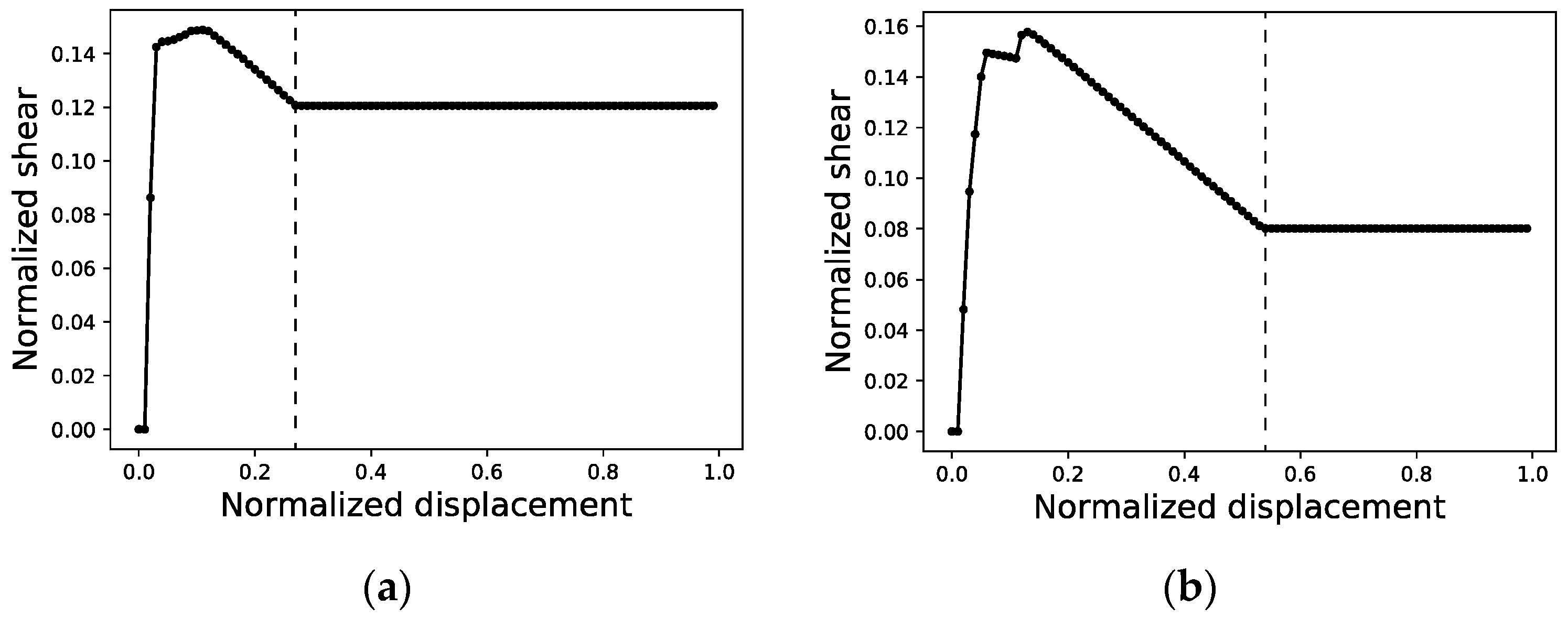
In order to arrange the data of each curve in a way that can be processed by the neural network, all curves in both the training and validation sets must be normalized (Figure 5) and defined by equal intervals in the displacement axis featuring the same number of points or segments. This normalization entails mapping the maximum shear value among all of the curves in the dataset to a value of 1.0 and all of the shear values of all curves will then be scaled proportionally. On the displacement axis, normalization means that only the curve with the maximum end displacement will be kept ‘as is’, while all others will see a set of horizontal segments appended to their last point to tally up with the number of segments of the maximum end displacement curve. Therefore, (i) a re-sampling of the curves is conducted, and (ii) shorter curves are completed with a stretch of constant shear value, as shown in Figure 6.
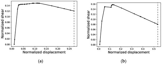
Figure 5.
Normalized capacity curves of structures #11 (a) and #34 (b) as returned from SAP2000.
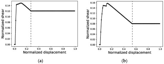
Figure 6.
Re-sampling of capacity curves of structures #11 (a) and #34 (b) with a resolution of 100 points and an interval of 0.01. Curve points to the left of the dashed line correspond to the original capacity curve after normalization. Curve points to the right are included in order to complete short curves with a stretch of constant shear value.
2.3.2. Curve Post-Processing
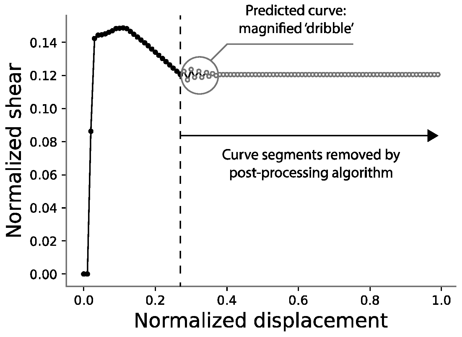
Once a curve is predicted, it is necessary to undo this horizontal stretch, so that the end point of the predicted curve can be obtained. Because of the stochastic nature of the neural network used in this study, the prediction of this horizontal part of the curve does not yield a perfectly straight line. Thus, it is necessary to design an algorithm capable of capturing it despite its irregularities, as shown in Figure 7. In this work, a simple algorithm was designed and implemented for this purpose with satisfactory results.
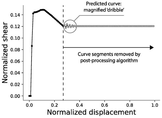
Figure 7.
Post-processing of predicted curves.
2.4. Artificial Neural Network
2.4.1. Loss Function and Error Measurements
The loss function establishes the metric against which the neural network learns. In [52], it was indicated that the root mean squared error and the mean absolute error are commonly used loss functions for the regression of continuous variables, i.e., the problem under study in the present paper. The root mean squared error (RMSE) is expressed as follows:
And the mean absolute error (MAE):
where (n) is the number of neurons of the output layer, (yi) are each one of the expected output values and (y′i) are the corresponding predicted values. This value will be calculated for each training sample and back-propagated into the network to serve as criteria for weight optimization. After intense training, the MAE value will be as low as possible (and thus the prediction error will be minimum). Both errors are similar, but, on the one hand, RMSE penalizes large errors more severely, whereas MAE provides a linear penalization; on the other hand, RMSE is less intuitive to interpret and is sensitive to the number of samples used for training. In [53], this is thoroughly analyzed and it is suggested that error metrics based on absolutes rather than squares can perform better in regression problems. For all of these reasons, MAE was chosen in this study over RMSE. Squared mean error is also very commonly used in neural networks, but was discarded due to poor results in preliminary testing.
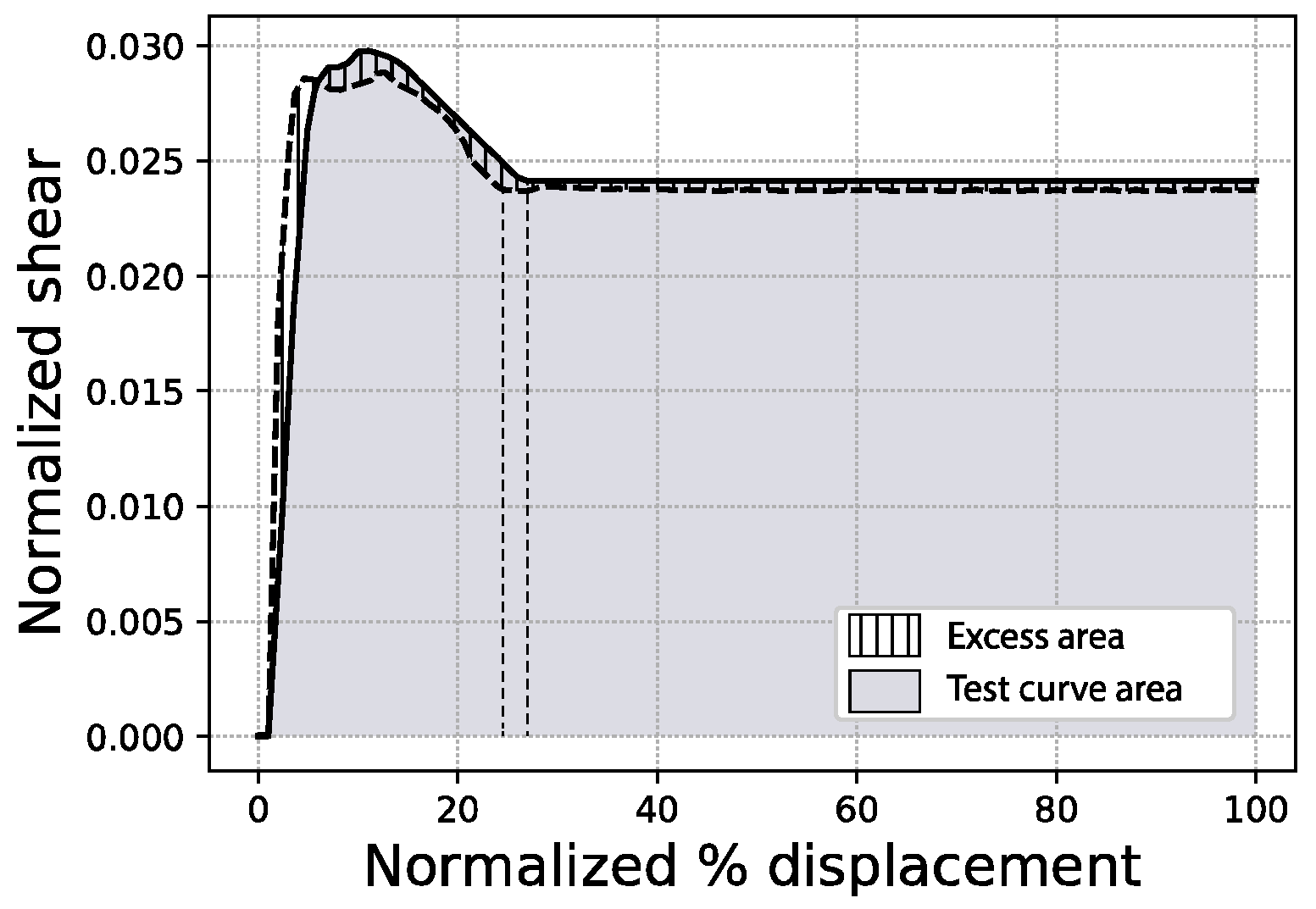
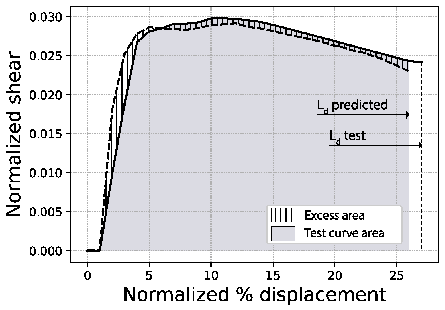
Because metrics like the mean absolute error might not be very intuitive visually, the results presented in this paper include three other expressions of the prediction error, just for the sake of clarity. First, the full area error % is defined as the percentage ratio between (i) the excess area enclosed in between the true (or test) capacity curve and the predicted curve, and (ii) the total area delimited by the test curve, as expressed in Figure 8. Second, the fitted area error % shares the same definition as above, but limits the areas to the lowest of the last displacement points of both curves (test and predicted), as in Figure 9. Additionally, in the figures that follow, the MAE is expressed as a percentage of the area calculated as the sum of all individual mean absolute errors for each curve point (100 points), times the interval between points (0.01).
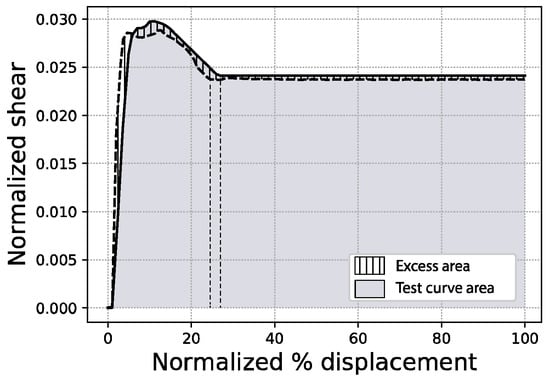
Figure 8.
Full area error scheme (sample #1062).
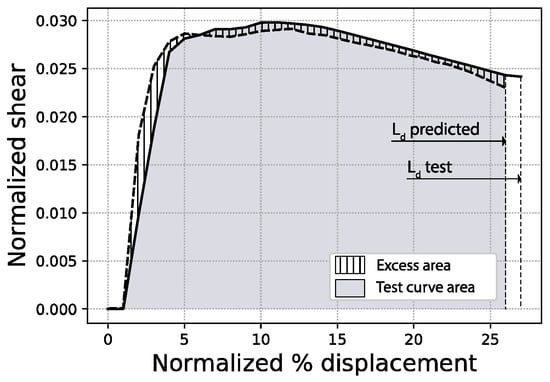
Figure 9.
Fitted area error and last displacement (Ld) error schemes (sample #1062).
Third and last, the last displacement error % refers to the prediction of the end point of the curve and is defined as the percentage ratio between (i) the absolute difference of both the predicted and true end points of the curve and (ii) the true end point, as shown in Figure 9. These measurements, especially the fitted area error % and the last displacement error % (Ld), allow the separate evaluation of (i) how well the curves fit one another in terms of shape and (ii) how well the network has predicted the end of the curve.
2.4.2. Network Architecture
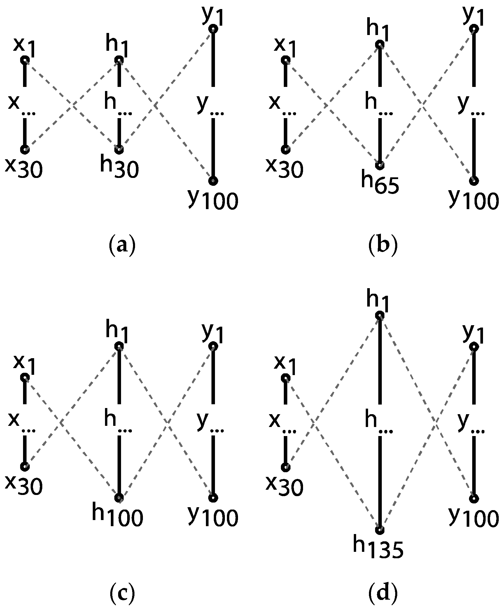
The first attempt at defining a network architecture is to implement a standard feedforward model. Because there is no theoretical methodology to establish the optimal configuration of the network [54], a stepped process, i.e., a grid search, is designed to determine the most appropriate architecture for the neural network model. More thorough methods such as genetic algorithm architecture optimization [55,56] will be explored in future work. In the first phase, a single layer network is set up with varying sizes of the hidden layer: (a) a hidden layer equal to the size of the input, (b) equal to the output layer, (c) a value in between and (d) larger than the output layer, as seen in Figure 10. This helps to assess what range of sizes in the hidden layer suits the problem best.
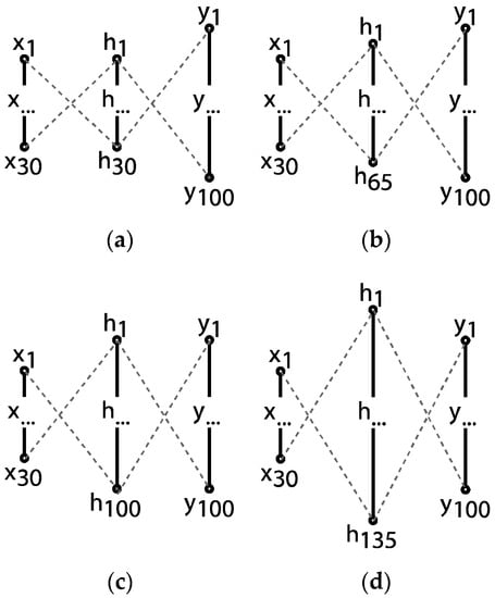
Figure 10.
Varying hidden layer sizes: (a) h1 = 30, (b) h1 = 65, (c) h1 = 100, (d) h1 = 135.
With this information at hand, another set of architectures of varying depth (i.e., a varying number of hidden layers) is evaluated. These layers use the previous size value as an initial or tentative layer size. It must be mentioned, though, that this value is only used temporarily, since more adjustments to the sizes of the hidden layers will be carried out later in the process.
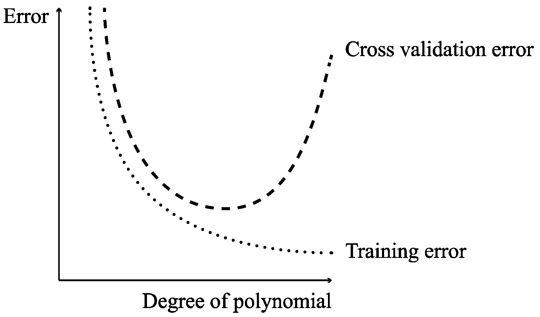
Deep neural architectures can be extremely powerful. When applied to regressions of continuous variables and time series (close examples to the datasets in this work), these models yield a great performance [57,58,59]. However, there is a trade-off between the complexity that a neural network can bring forward and the overfitting of the model to the data, as shown in Figure 11.
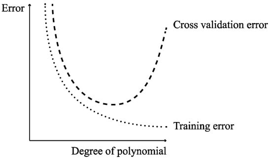
Figure 11.
Model complexity vs training and validation errors (overfitting problem).
Due to overfitting, deep architectures may perform very well on the training samples, but poorly on the validation data. To test out the interplay of these factors, three initial architectures are presented according primarily to the number of hidden layers (depth). Below, Figure 12 shows a diagram of these schemes.
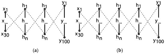
Figure 12.
Varying depths in network architecture: 2 (a) and 3 (b) hidden layers.
In both Figure 10 and Figure 12, (x) represents the input neurons of the network. As seen in previous sections, the total number of inputs for the network is fixed to 30, as this matches the number of parameters that have been used to generate the buildings. Then, (h) represents the hidden layers in the model. An initial size is temporarily set at 65, as it is the best-performing size in a preliminary and intuitive evaluation, but more refined values will be explored later. Finally, (y) is the output layer, which corresponds to the values of the capacity curves that the network is aiming to predict. The size of this output layer has a strong impact on the performance of the learning process. Small sizes in this layer reduce the level of difficulty of the predictions; however, a valid resolution for the curves must be ensured. For this reason, the number of neurons in the output layer is initially set at 100, because on the one hand, it provides enough resolution to graph the capacity curve as discussed, and on the other hand, it is slightly higher than the maximum number of points present in the original capacity curves retrieved from SAP2000. However, variations in this output size will also be discussed in the following sections.
From this outset, the main algorithms of the network will be explored, namely, the activation functions that are implemented in each layer (which may be considered an algorithm when viewed as a whole) and the error optimization algorithm.
2.4.3. Activation Function
The activation function maps the output of an artificial neuron to a desired value range. Neural networks are very sensitive to this function, and there are many possible activation functions used in neural networks, so which one fits the problem best must be determined. In [60], it was observed that a hyperbolic tangent (tanh) is a common activation function applied to the hidden layers of a neural network for similar problems as the one being dealt with in this study, whereas sigmoid activations are commonly used for the output layer (as they map from 0 to 1). For this reason, both tanh and sigmoid activation functions were tested in the hidden and output layers, respectively. Alternatively, at the fine-tuning phase, a rectified linear unit (ReLU) activation was also tested due to its common use in deep neural architectures [61], but no positive results were obtained.
2.4.4. Optimizer
A preliminary choice for the optimization algorithm was the stochastic gradient descent (SGD), which is the basic algorithm for neural network training [62]. Nevertheless, at a later stage, a second algorithm was tested, namely the Adadelta optimizer [63], which is a variant of the SGD that presents a novel per-dimension learning rate method for gradient descent by dynamically adapting over time. The application of this optimization algorithm did not improve the error rate obtained using the SGD.
2.4.5. Preliminary Adjustment of Stochastic Gradient Descent (SGD) Parameters
As explained in the methodology section, the first objective is to fix the architecture of the network and the parameters of the optimizer algorithm. In order to test various architectures reliably, it is necessary to find a satisfactory set of parameters that guide the back-propagation of the error. For this purpose, a simple initial architecture was defined.
The initial conditions for the preliminary SGD adjustment are shown in Table 3. The SGD was adjusted through the following parameters: Learning rate (Lr), Decay and Momentum (M). The results were measured against the validation set using the mean absolute error (Table 4 and Figure 13).
Table 3.
Initial conditions for preliminary Stochastic Gradient Descent (SGD) adjustment.
Table 4.
Experimentation and results of preliminary SGD adjustment.
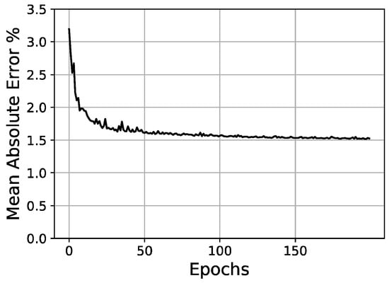
Figure 13.
Loss/epochs graph with selected SGD values of preliminary adjustment.
2.4.6. Network Architecture Configuration
Once the parameters of the optimizer have been set, it is then possible to test different network architectures more effectively. In these tests, a hyperbolic tangent (tanh) activation in the hidden layers and a sigmoid activation function in the output layer were fixed. In Table 5, the initial conditions for network architecture variations are shown. Then, Table 6 and Figure 14, Figure 15 and Figure 16 present the tests and results of the network architecture, showing the different variations over the hidden layers. In Table 7, the results of the curve resolution (size of output layer) are listed.
Table 5.
Initial conditions for network architecture variations.
Table 6.
Results of hidden layer/s architecture.
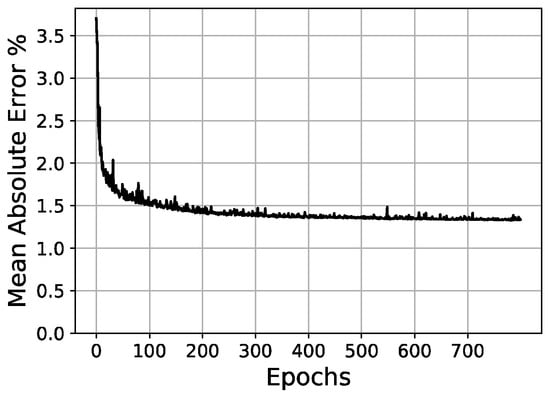
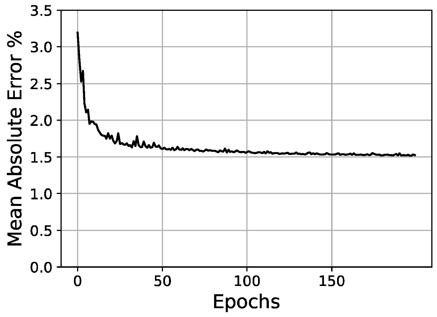
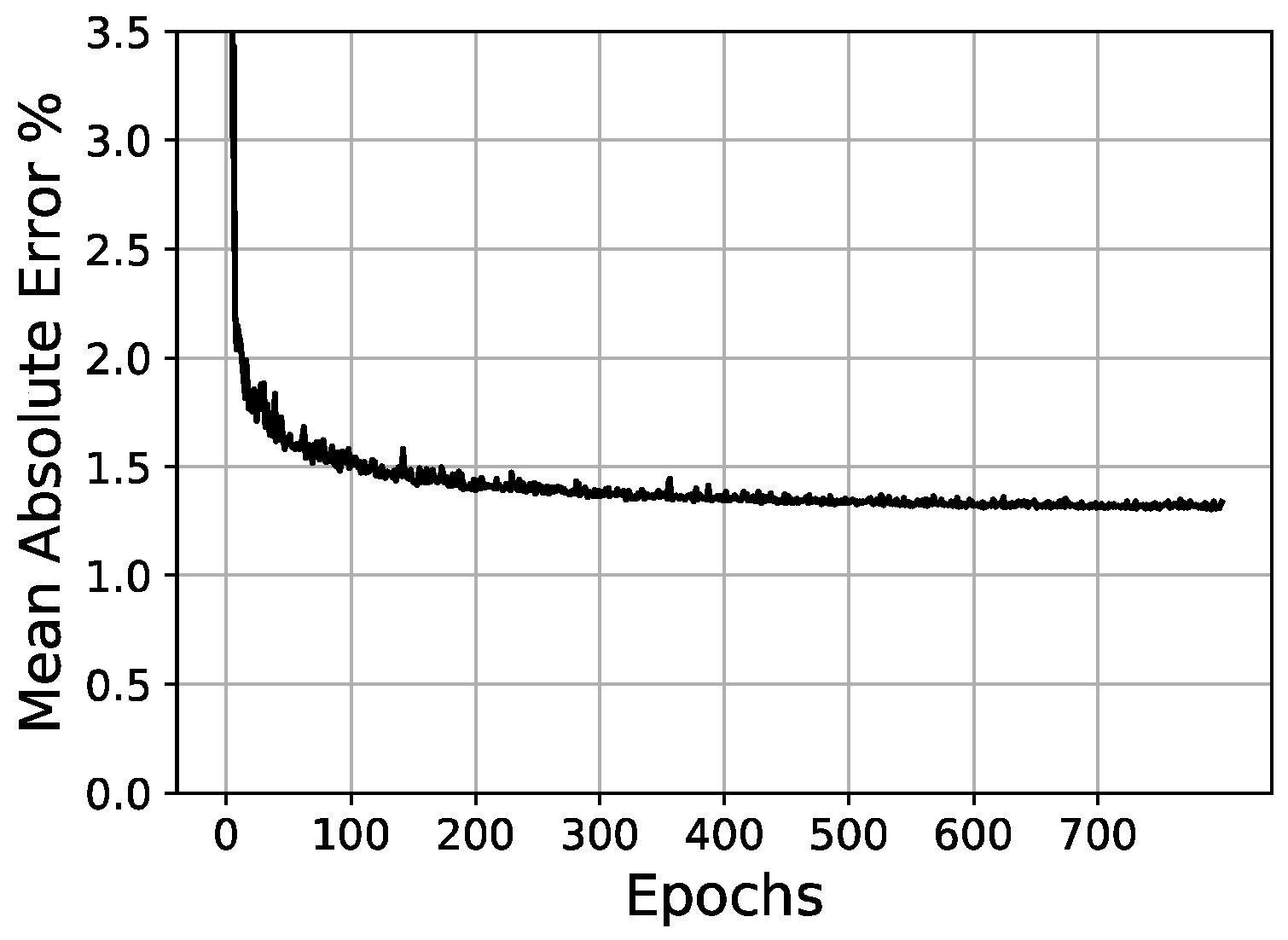
Figure 14.
Validation loss/epochs graph for 30-205-100 scheme (one hidden layer).
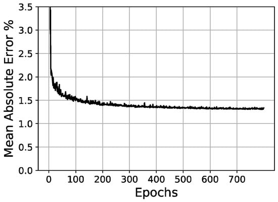
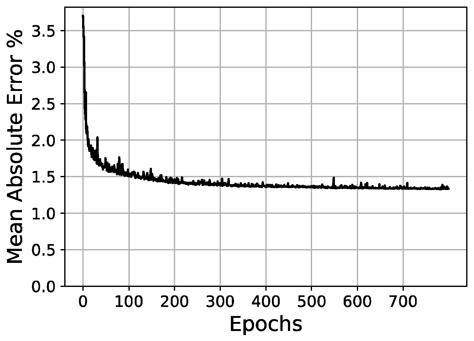
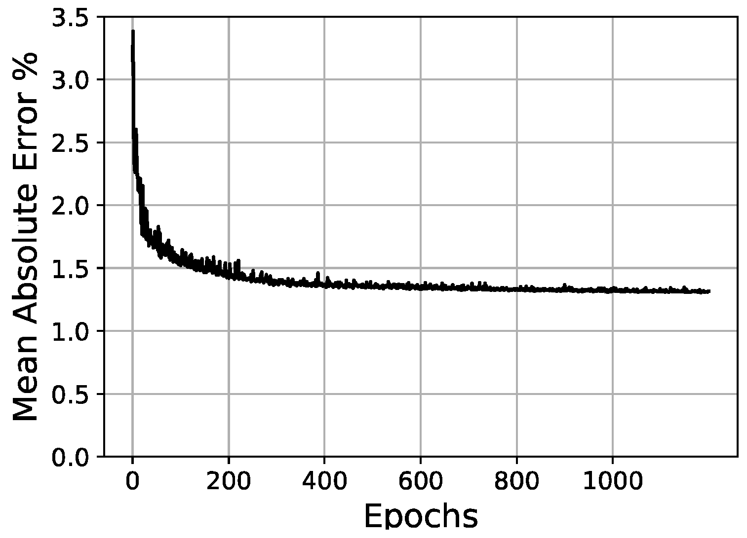
Figure 15.
Validation loss/epochs graph for 30-100-100-100 scheme (two hidden layers).

Figure 16.
Validation loss/epochs graph for 30-30-30-65-100 scheme (three hidden layers).
Table 7.
Results of curve resolution (output layer architecture).
2.4.7. Network Parameter Fine-Tuning
After obtaining the best error rates for all of the configurations tested, a final architecture of 30-65-65-100 was selected. From this setup, a more refined set of variations was executed. These variations included a second round of SGD optimizer parameters, as well as an attempt on the Adadelta optimizer, ReLU activation for hidden layers, and different batch sizes. The number of training epochs is always prolonged until the error does not improve significantly.
The initial conditions for the network parameter fine-tuning are presented in Table 8. The experimentation and results of the network parameter fine-tuning are shown in Table 9. Finally, the support data for the selected samples can be consulted in Table A1 and Table A2 of the Appendix A.
Table 8.
Initial setup for network parameter fine-tuning.
Table 9.
Network parameter fine-tuning results.
3. Results
Following the experimentation, a final configuration of the network was achieved, which is detailed in Table 10. Specific examples of the results are provided and shown in the Appendix A.
Table 10.
Final network architecture.
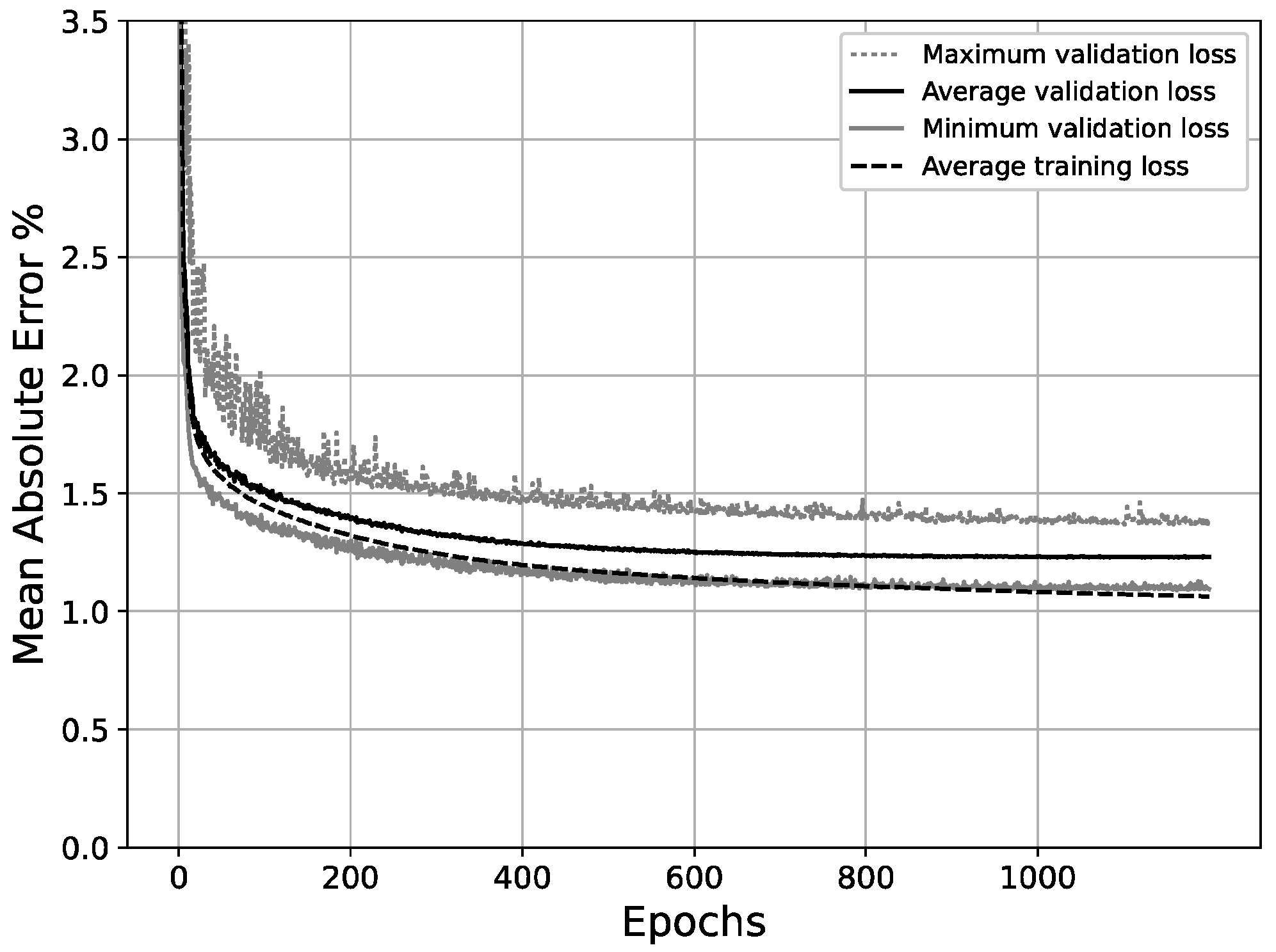
With the final network configuration presented, after 1200 epochs, the average validation MAE across 60 random splits between training and validation sets was 0.0123 (1.23%). A graph plotting the MAE (%)/epoch progress for the minimum, maximum and average results out of the randomized splits is shown in Figure 17. Additionally, the RMSE was also calculated in order to draw comparisons with other work, yielding a value of 0.0134 and following a very similar distribution to the MAE.

Figure 17.
Average, maximum and minimum validation loss, and average training loss/epochs for final scheme (30-65-65-100).
However, as can be observed in Figure 17, the best balance between the validation error and the overfitting ratio is achieved around epoch #700, where the average training and validation MAE are 0.0112 and 0.0124, respectively. This couplet of values makes up for an overfitting ratio of 0.904, which lies within an acceptable range [52]. Beyond this point, the validation error does not improve significantly, while the divergence between training and validation errors increases at a steady pace, thus increasing the overfitting ratio without a substantial gain in the validation accuracy. Table 11 shows the evolution of the average overfitting ratio across epochs.
Table 11.
Overfitting ratio across epochs.
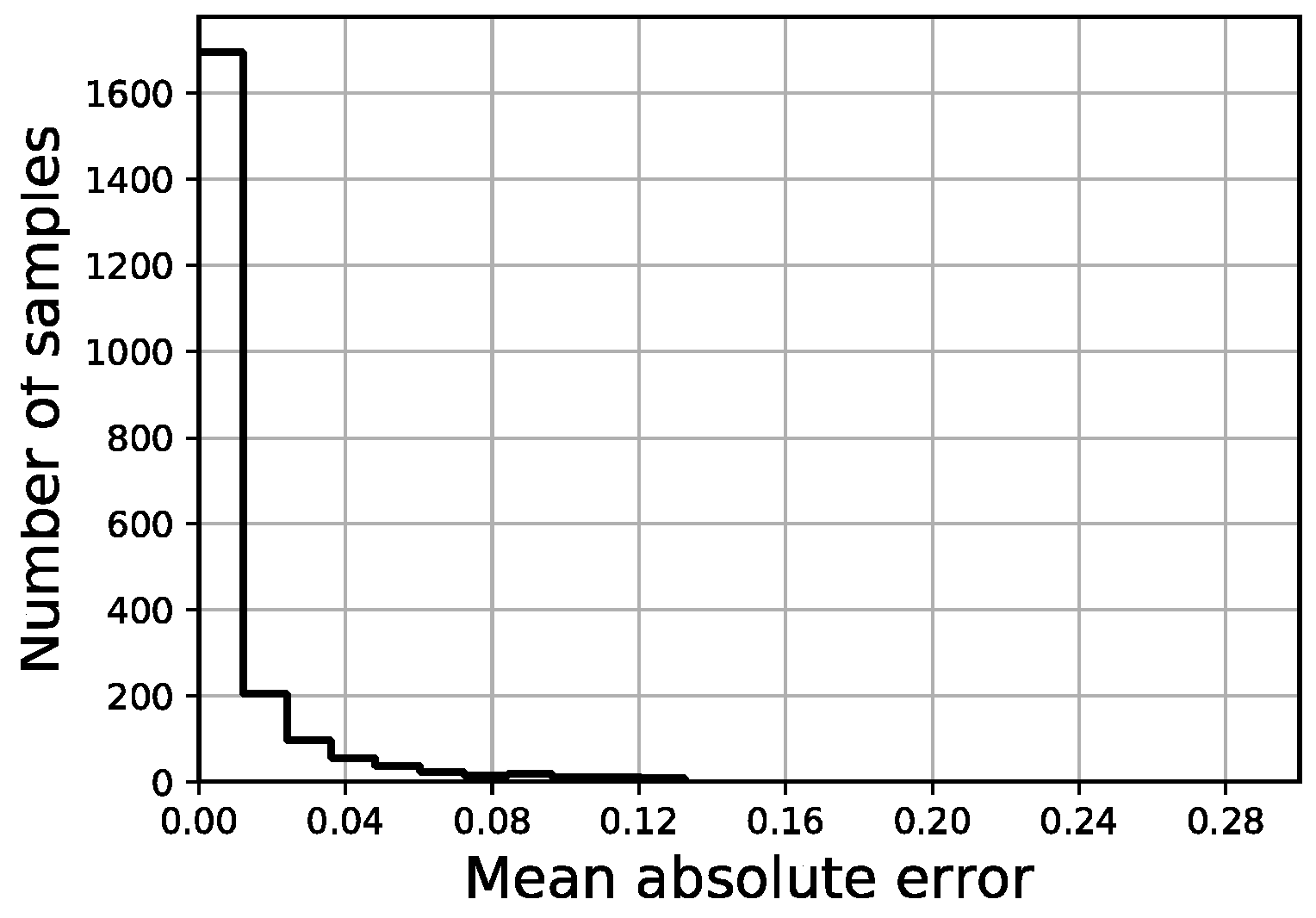
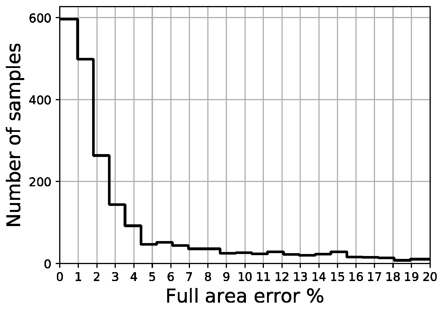
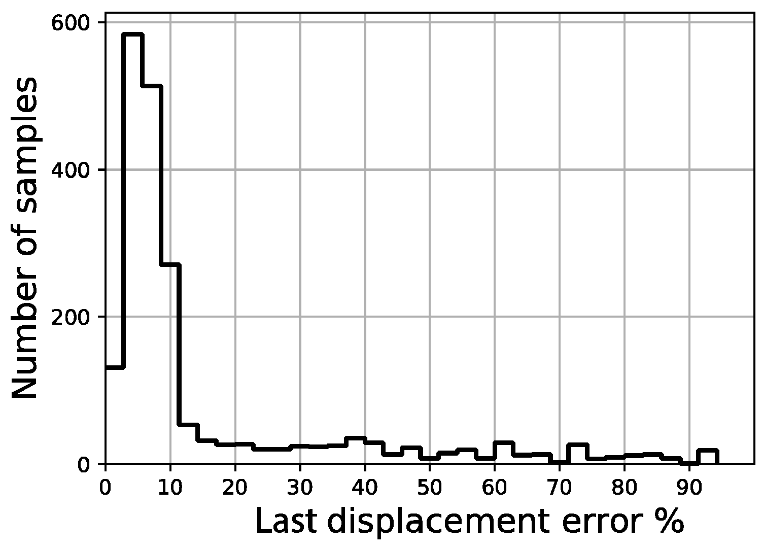
The distribution of the four error indicators defined in the scope of this work (MAE, full area error, fitted area error and Ld) are shown in Figure 18, Figure 19, Figure 20 and Figure 21, respectively. The average fitted area error obtained for capacity curves is 2.35%, while the full area error is 2.65%. Last displacement error (Ld) is 20.81% on average.
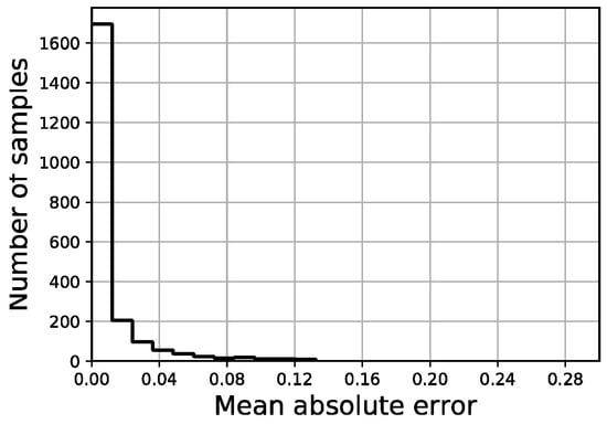
Figure 18.
MAE distribution of validation set.

Figure 19.
Full area error distribution of validation set.
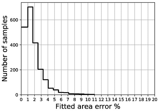
Figure 20.
Fitted area error distribution of validation set.

Figure 21.
Last displacement error distribution of validation set.
Out of a total of 2200 samples in the validation set, less than 50 samples present a fitted area error above 5.0% and there are no samples above 11.0%, while more than 1200 samples remain below the 2% threshold. Regarding the last displacement error, although most of the samples display an error below 10%, there is a constant spread of this error along the percentage axis all the way up to 100%.
To illustrate what these errors account for in visual terms, specific samples of curves have been graphed for three representative error values within the error distributions obtained. For the fitted area error, Figure 22 shows a sample with an error below 1%, while Figure 23 corresponds to a sample with an error close to the average value of the distribution (2.35%), and Figure 24 an error close to 5%, which represents the largest error range containing a meaningful number of samples (at least 10). More data on these specific samples can be consulted in Table A1 of the Appendix A.

Figure 22.
Fitted area error < 1.0% validation sample #1355.

Figure 23.
Fitted area error ~2.35% validation sample #1547.
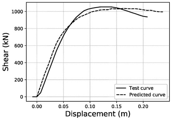
Figure 24.
Fitted area error ~5.0% validation sample #147.
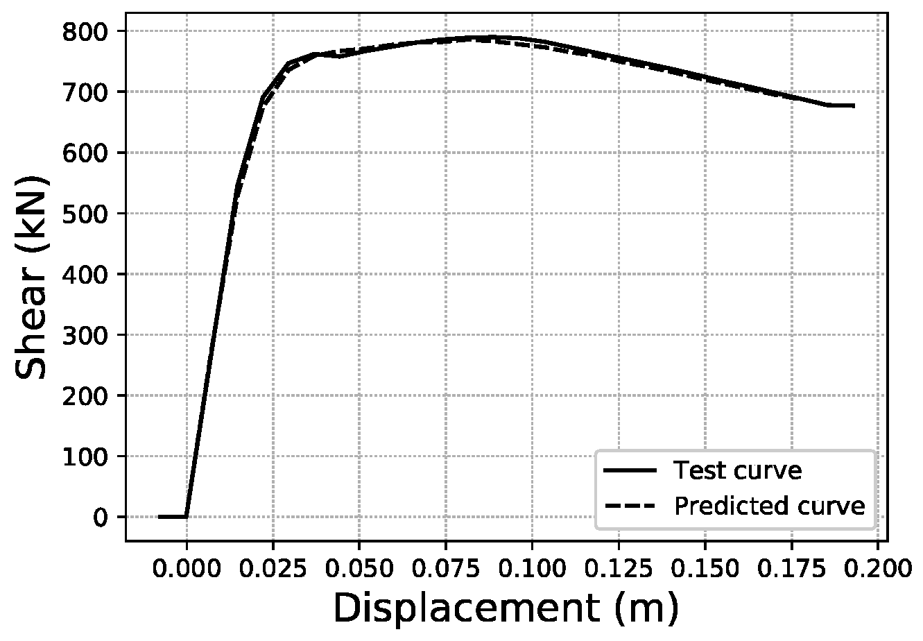
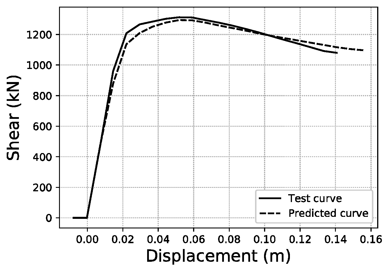
For the last displacement error (Ld), the thresholds chosen to provide a visual illustration are Ld < 5%, Ld ~21.32% (average of the distribution) and Ld ~60%, as shown in Figure 25, Figure 26 and Figure 27. More data on these specific samples can be consulted in Table A2 of the Appendix A.
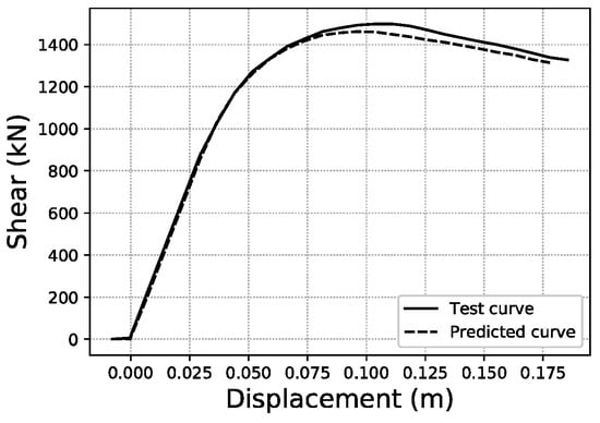
Figure 25.
Ld < 5.0% validation sample #639.
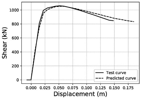
Figure 26.
Ld ~21.32% validation sample #1971.
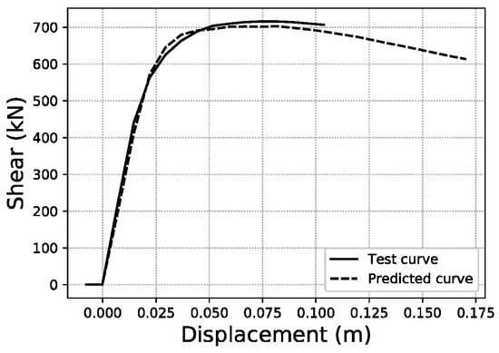
Figure 27.
Ld ~60.0% validation sample #1926.
4. Discussion of Results
The tests on different network architectures yielded the best results for configurations that featured two hidden layers; in particular, the scheme that delivered the best results was 30-65-65-100, as shown in Table 6. Architectures with only one hidden layer returned better results with larger sizes, but still not as competitive as the latter. The fact that the network clearly performs better when increasing its complexity accounts for the level of difficulty of the predictions. However, as illustrated previously in Figure 11, after a certain point, increasing the complexity of the model does not improve the results due to overfitting. Perhaps, with an even larger training set, these deeper architectures may improve the results presented in this paper, thus leaving room for future work.
Regarding the size of the output layer, and rather counter-intuitively, smaller sizes of curve resolution did not improve the metrics. An initial output layer size of 100 was set because it was considered to have enough resolution for the problem at hand while not being excessively large for training. Interestingly, lowering this value proved detrimental, while eventually increasing its size up to 135 yielded equally accurate results (see Table 7). This can be explained by the fact that lower resolutions are less loyal to the calculation algorithms within the engineering software that produced the validation set of capacity curves (SAP2000), and since neural networks perform best with clear patterns, lower resolutions introduce harmful noise into the training process.
At the fine-tuning stage, batch sizes played an important role in maximizing the curve prediction accuracy. Although there may be some disagreement on the regularizing effect of the batch size [64,65], in these experiments, it was found that larger batch sizes can prevent overfitting by regularizing the network to some extent, because the loss values are averaged for all elements in the batch and then back-propagated to adjust the weights and biases of the model. Table 9 shows how the lowest batch sizes had very good training results, but lagged when tested against the validation set, thus displaying a more acute overfitting. The best-performing batch size tested was of 24 samples.
Beyond the exploration of network parameters, it is important to note that the one critical factor in achieving the results discussed above was the size of the dataset. Initial attempts not accounted for in this text were carried out with 2000 samples and delivered poor results. The increase to 7000 samples saw the largest impact in accuracy among all of the different options and parameters tested in that first round of experiments. However, it is important to observe that these results should be tested and validated on real cases to measure the impact of the modeling assumptions (like the lack of infill panels) established in this method. Additionally, there are several uncertainties implicit in the results from the model that need to be explored further, such as the actual properties of the materials that have been modeled according to industry regulations, but are not based on empiric material surveys on the ground.
Although this research is centered on its applicability to a very broad range of structures, the results achieved still compare quite well to other work previously discussed in this paper. In [26], the maximum inter-story drift ratio (MIDR) was predicted using different ANN models. The best results featured the prediction of MIDR values with an error between 1.5% and 2%. Despite the obvious difference of the parameters being measured, the average fitted area error of 2.35% achieved in the present study remains within close range to those results. Another interesting point of comparison is the work of Pérez Ramírez et al. [27], where a recurrent neural network model with Bayesian training and mutual information is employed to estimate the acceleration response spectrum of buildings. In this case, the model also aims to predict a response curve and, therefore, a better comparison can be established. Their results show the prediction accuracy of the network for a large residential building and a scaled model of a five-story steel structure under both seismic action and ambient vibrations. For the 30th floor of the residential building, the lowest RMSE values were 0.1789 and 0.1827 for moderate and high-level seismic excitations, respectively. These results are less accurate than the RMSE of 0.0134 achieved in the present work, but, of course, predicting the vibration response of a high-rise building is also a very tough challenge.
Future Work
In the short term, it may be interesting to include the use of genetic algorithms to evolve an even more optimal network architecture. Additionally, a comparison with other regression methods or machine learning approaches would be desirable to contextualize the results presented in this paper, while in the long term, it might be interesting to explore a similar approach with (i) dynamic nonlinear analysis, e.g., time history analysis, (ii) irregular structures and high-rise buildings with higher vibration modes and (iii) a wider variation of sectional and material properties. It should also be observed that this work has followed the capacity spectrum method from Eurocode 8, which is proven to work well with low-rise structures. However, a research effort to predict capacity curves under a set of strong earthquakes that can produce greater nonlinearities would extend the applicability of the method presented in this paper. All of these cases (dynamic analysis, high-rise buildings and stronger earthquakes) pose a greater challenge in terms of machine learning and may require the use of more specialized neural network architectures. In this regard, because capacity curves can be regarded as time-dependent time series, network models better suited to handle dynamic inputs, such as recurrent neural networks [66,67], should be explored.
5. Conclusions
A method based on artificial neural networks to estimate the capacity curves of low-rise RC buildings was developed and implemented. In the methodology presented, no modeling of the specific building is required. Curves can be estimated with an average curve-area fitting above 97.6%, only requiring the basic geometric parameters of the building to be specified.
As a first implementation, a typology of prismatic RC buildings was defined and a training set of more than 7000 structures was parametrically generated. The capacity curves of these models were obtained by means of push-over analysis using SAP2000 software.
The proposed method is fit for the accurate assessment of the seismic vulnerability of regular low-rise RC buildings almost instantly. It provides a fast and reliable alternative for the calculation of capacity curves when detailed information of the building is unavailable, but basic data are available (number of spans, span dimensions, beam and column profiles and slab thickness). It may also provide a fast and robust alternative when, due to the large volume of buildings to be assessed, it is not feasible to engage in individual modeling. While current macro-seismic approaches address these issues, their accuracy is in no way comparable. This feature can be very relevant in the light of urban scenarios where the seismic vulnerability of a great number of buildings needs to be assessed. The resulting trained network can be used by emergency services and other government bodies as a decision-making tool for prevention purposes (targeted retrofitting interventions, for example) and, after a seismic event, for quick and effective relief action.
The main conclusions of the research presented in this paper are the following:
- -
- ANN provide an accurate approximation method for the nonlinear static push-over calculation of low-rise structures within a wide range of sizes and geometric configurations.
- -
- The accuracy of the method successfully addresses the shortcomings of current macro-seismic approaches, while remaining fast and efficient.
- -
- Stress-deformation curves in a plastic regime can be predicted with ANN in one go for entire buildings using only basic geometric parameters. For low-rise structures, this work achieves a curve area error below 2.7% and a resolution of up to 100 points.
- -
- The relative simplicity of the ANN architecture required to predict the capacity curves of low-rise buildings makes a strong case for the future research of high-rise structures using deeper networks and larger datasets.
Author Contributions
Conceptualization, J.d.-M.-R. and A.M.-E.; data curation, J.d.-M.-R.; formal analysis, J.d.-M.-R.; funding acquisition, A.M.-E. and J.M.C.-E.; investigation, J.d.-M.-R., M.-V.R.-G.-C., B.Z.-B., M.-L.S.-V. and E.R.-S.; methodology, J.d.-M.-R. and A.M.-E.; project administration, A.M.-E. and J.M.C.-E.; resources, A.M.-E.; software, J.d.-M.-R.; supervision, A.M.-E.; validation, J.d.-M.-R.; visualization, J.d.-M.-R., M.-V.R.-G.-C. and E.R.-S.; writing—original draft, J.d.-M.-R.; writing—review and editing, J.d.-M.-R., A.M.-E., M.-V.R.-G.-C. and B.Z.-B. All authors have read and agreed to the published version of the manuscript.
Funding
The grant provided by the Spanish National Project SIMRIS (A seismic risk simulator and a real-time evaluating tool in case of earthquake for residential buildings of the Iberian Peninsula) is acknowledged. The grant provided by the Instituto Universitario de Arquitectura y Ciencias de la Construcción is also acknowledged.
Institutional Review Board Statement
Not applicable.
Informed Consent Statement
Not applicable.
Data Availability Statement
Not applicable.
Acknowledgments
The authors wish to thank Fernando Sancho Caparrini for his kind support on the machine learning aspects of the paper.
Conflicts of Interest
The authors declare no conflict of interest.
Appendix A
Table A1.
Error data and input parameters for selected samples.
Table A1.
Error data and input parameters for selected samples.
| Sample #147 | Sample #1547 | Sample #1355 | ||
|---|---|---|---|---|
| Error data | MAE | 0.0097 | 0.0048 | 0.00072 |
| Full area error | 5.21% | 2.13% | 0.49% | |
| Fitted area error | 5.48% | 2.27% | 0.80% | |
| Ld error | 13.3% | 9.52% | 7.14% | |
| Input parameters | Spans in X (m) | 6.4, 5.4 | 6.43, 5.39 | 6.7, 4.1, 4.8, 6.9, 4.3, 4.5, 6.6 |
| Spans in Y (m) | 5.2, 4.3, 5.8, 3.1, 5.3, 3.2, 4.1 | 4, 4.5, 4.8, 3, 3.3, 3.2, 5.3, 4.9, 5.4 | 3.2, 4.8 | |
| Spans in Z (m) | 0.7, 3.5, 3.3, 3.4 | 0.7, 3.4, 3.2, 3 | 0.6, 3.9, 3.1 | |
| Wide load B. B.? | Yes | No | No | |
| Load B. B. dim | 60 × 30 cm | 30 × 60 cm | 30 × 60 cm | |
| Non-load B. B. dim | 30 × 30 cm | 30 × 30 cm | 30 × 30 cm | |
| Supports dim | 30 × 30 cm | 30 × 30 cm | 30 × 30 cm | |
| Slab thickness | 30 cm | 30 cm | 30 cm |
Table A2.
Error data and input parameters for selected samples.
Table A2.
Error data and input parameters for selected samples.
| Sample #1926 | Sample #1971 | Sample #639 | ||
|---|---|---|---|---|
| Error data | MAE | 0.0179 | 0.0065 | 0.0074 |
| Full area error | 12.44% | 3.62% | 2.75% | |
| Fitted area error | 2.21% | 2.26% | 1.99% | |
| Ld error | 56.2% | 22.7% | 3.70% | |
| Input parameters | Spans in X (m) | 7.7, 4.5, 5.6, 4.9 | 6.1, 5.2 | 6.3, 4.5, 4.2, 5.9 |
| Spans in Y (m) | 4.8, 5.6, 5.5 | 3.8, 4.8, 4.7, 5.3, 5.0, 5.2, 5.1 | 5.1, 4.6, 4.3, 5.3, 4.8, 4.7 | |
| Spans in Z (m) | 0.6, 3.9, 3.1 | 0.7, 3.4, 3.1, 3.2 | 0.6, 3.65, 3.35, 3.4 | |
| Wide load B. B.? | Yes | No | Yes | |
| Load B. B. dim | 60 × 30 cm | 30 × 60 cm | 60 × 30 cm | |
| Non-load B. B. dim | 30 × 30 cm | 30 × 30 cm | 30 × 30 cm | |
| Supports dim | 30 × 30 cm | 30 × 30 cm | 30 × 30 cm | |
| Slab thickness | 30 cm | 30 cm | 30 cm |
References
- Sá, L.F.; Morales-Esteban, A.; Neyra, P.D. A Seismic Risk Simulator for Iberia. Bull. Seism. Soc. Am. 2016, 106, 1198–1209. [Google Scholar] [CrossRef]
- Antonucci, A.; Rovida, A.; D’Amico, V.; Albarello, D. Integrating macroseismic intensity distributions with a probabilistic approach: An application in Italy. Nat. Hazards Earth Syst. Sci. 2021, 21, 2299–2311. [Google Scholar] [CrossRef]
- Valente, M.; Milani, G. Seismic assessment of historical masonry towers by means of simplified approaches and standard FEM. Constr. Build. Mater. 2016, 108, 74–104. [Google Scholar] [CrossRef]
- Barbieri, G.; Biolzi, L.; Bocciarelli, M.; Fregonese, L.; Frigeri, A. Assessing the seismic vulnerability of a historical building. Eng. Struct. 2013, 57, 523–535. [Google Scholar] [CrossRef]
- Candia, G.; Jaimes, M.; Arredondo, C.; De La Llera, J.C.; Favier, P. Seismic Vulnerability of Wine Barrel Stacks. Earthq. Spectra 2016, 32, 2495–2511. [Google Scholar] [CrossRef]
- Mouroux, P.; Le Brun, B. Presentation of RISK-UE Project. Bull. Earthq. Eng. 2006, 4, 323–339. [Google Scholar] [CrossRef]
- Barbat, A.H.; Carreño, M.L.; Pujades, L.G.; Lantada, N.; Cardona, O.D.; Marulanda, M.C. Seismic vulnerability and risk evaluation methods for urban areas. A review with application to a pilot area. Struct. Infrastruct. Eng. 2010, 6, 17–38. [Google Scholar] [CrossRef]
- Fiore, A.; Sulpizio, C.; DeMartino, C.; Vanzi, I.; Biondi, S.; Fabietti, V. Seismic vulnerability assessment of historical centers at urban scale. Int. J. Arch. Heritage 2017, 12, 257–269. [Google Scholar] [CrossRef]
- Simões, A.; Bento, R.; Cattari, S.; Lagomarsino, S. Seismic performance-based assessment of “Gaioleiro” buildings. Eng. Struct. 2014, 80, 486–500. [Google Scholar] [CrossRef]
- Milosevic, J.; Cattari, S.; Bento, R. Definition of fragility curves through nonlinear static analyses: Procedure and application to a mixed masonry-RC building stock. Bull. Earthq. Eng. 2020, 18, 513–545. [Google Scholar] [CrossRef] [Green Version]
- Gautam, D.; Adhikari, R.; Rupakhety, R.; Koirala, P. An empirical method for seismic vulnerability assessment of Nepali school buildings. Bull. Earthq. Eng. 2020, 18, 5965–5982. [Google Scholar] [CrossRef]
- Çavdar, Ö.; Bayraktar, A. Pushover and nonlinear time history analysis evaluation of a RC building collapsed during the Van (Turkey) earthquake on October 23, 2011. Nat. Hazards 2013, 70, 657–673. [Google Scholar] [CrossRef]
- Mwafy, A.; Elnashai, A. Static pushover versus dynamic collapse analysis of RC buildings. Eng. Struct. 2001, 23, 407–424. [Google Scholar] [CrossRef]
- Lee, S.-C.; Ma, C.-K. Time history shaking table test and seismic performance analysis of Industrialised Building System (IBS) block house subsystems. J. Build. Eng. 2021, 34, 101906. [Google Scholar] [CrossRef]
- Maleska, T.; Beben, D.; Nowacka, J. Seismic vulnerability of a soil-steel composite tunnel—Norway Tolpinrud Railway Tunnel Case Study. Tunn. Undergr. Space Technol. 2021, 110, 103808. [Google Scholar] [CrossRef]
- Pang, R.; Xu, B.; Zhou, Y.; Song, L. Seismic time-history response and system reliability analysis of slopes considering uncertainty of multi-parameters and earthquake excitations. Comput. Geotech. 2021, 136, 104245. [Google Scholar] [CrossRef]
- Pilarska, D.; Maleska, T. Numerical Analysis of Steel Geodesic Dome under Seismic Excitations. Materials 2021, 14, 4493. [Google Scholar] [CrossRef]
- Asteris, P.G.; Nozhati, S.; Nikoo, M.; Cavaleri, L.; Nikoo, M. Krill herd algorithm-based neural network in structural seismic reliability evaluation. Mech. Adv. Mater. Struct. 2019, 26, 1146–1153. [Google Scholar] [CrossRef]
- Wang, Z.; Pedroni, N.; Zentner, I.; Zio, E. Seismic fragility analysis with artificial neural networks: Application to nuclear power plant equipment. Eng. Struct. 2018, 162, 213–225. [Google Scholar] [CrossRef] [Green Version]
- Zhang, R.; Liu, Y.; Sun, H. Physics-guided convolutional neural network (PhyCNN) for data-driven seismic response modeling. Eng. Struct. 2020, 215, 110704. [Google Scholar] [CrossRef]
- Ahmed, B.; Mangalathu, S.; Jeon, J.-S. Seismic damage state predictions of reinforced concrete structures using stacked long short-term memory neural networks. J. Build. Eng. 2022, 46, 103737. [Google Scholar] [CrossRef]
- Yuan, X.; Chen, G.; Jiao, P.; Li, L.; Han, J.; Zhang, H. A neural network-based multivariate seismic classifier for simultaneous post-earthquake fragility estimation and damage classification. Eng. Struct. 2022, 255, 113918. [Google Scholar] [CrossRef]
- Kim, M.; Song, J. Near-Real-Time Identification of Seismic Damage Using Unsupervised Deep Neural Network. J. Eng. Mech. 2022, 148, 04022006. [Google Scholar] [CrossRef]
- Soleimani, F.; Liu, X. Artificial neural network application in predicting probabilistic seismic demands of bridge components. Earthq. Eng. Struct. Dyn. 2021, 51, 612–629. [Google Scholar] [CrossRef]
- Huo, H.; Zhou, L.; Wang, Y.; Zhang, T. A Method for Predicting Seismic Stress and Deformation of Circular Tunnels Based on BP Artificial Neural Network. Lect. Notes Civ. Eng. 2021, 126, 369–376. [Google Scholar] [CrossRef]
- Morfidis, K.; Kostinakis, K. Approaches to the rapid seismic damage prediction of r/c buildings using artificial neural networks. Eng. Struct. 2018, 165, 120–141. [Google Scholar] [CrossRef]
- Perez-Ramirez, C.A.; Amezquita-Sanchez, J.P.; Valtierra-Rodriguez, M.; Adeli, H.; Dominguez-Gonzalez, A.; Romero-Troncoso, R.J. Recurrent neural network model with Bayesian training and mutual information for response prediction of large buildings. Eng. Struct. 2019, 178, 603–615. [Google Scholar] [CrossRef]
- Asim, K.M.; Martínez-Álvarez, F.; Basit, A.; Iqbal, T. Earthquake magnitude prediction in Hindukush region using machine learning techniques. Nat. Hazards 2017, 85, 471–486. [Google Scholar] [CrossRef]
- Panakkat, A.; Adeli, H. Recurrent Neural Network for Approximate Earthquake Time and Location Prediction Using Multiple Seismicity Indicators. Comput. Civ. Infrastruct. Eng. 2009, 24, 280–292. [Google Scholar] [CrossRef]
- Ruggieri, S.; Cardellicchio, A.; Leggieri, V.; Uva, G. Machine-learning based vulnerability analysis of existing buildings. Autom. Constr. 2021, 132, 103936. [Google Scholar] [CrossRef]
- Moayedi, H.; Mosallanezhad, M.; Rashid, A.S.A.; Jusoh, W.A.W.; Muazu, M.A. A systematic review and meta-analysis of artificial neural network application in geotechnical engineering: Theory and applications. Neural Comput. Appl. 2020, 32, 495–518. [Google Scholar] [CrossRef]
- Alizadeh, M.; Ngah, I.; Hashim, M.; Pradhan, B.; Pour, A.B. A Hybrid Analytic Network Process and Artificial Neural Network (ANP-ANN) Model for Urban Earthquake Vulnerability Assessment. Remote Sens. 2018, 10, 975. [Google Scholar] [CrossRef] [Green Version]
- Nguyen, Q.H.; Ly, H.-B.; Nguyen, T.-A.; Phan, V.-H.; Nguyen, L.K.; Tran, V.Q. Investigation of ANN architecture for predicting shear strength of fiber reinforcement bars concrete beams. PLoS ONE 2021, 16, e0247391. [Google Scholar] [CrossRef] [PubMed]
- Won, J.; Shin, J. Machine Learning-Based Approach for Seismic Damage Prediction Method of Building Structures Considering Soil-Structure Interaction. Sustainability 2021, 13, 4334. [Google Scholar] [CrossRef]
- Kwag, S.; Hahm, D.; Kim, M.; Eem, S. Development of a Probabilistic Seismic Performance Assessment Model of Slope Using Machine Learning Methods. Sustainability 2020, 12, 3269. [Google Scholar] [CrossRef] [Green Version]
- Arslan, M.H. An evaluation of effective design parameters on earthquake performance of RC buildings using neural networks. Eng. Struct. 2010, 32, 1888–1898. [Google Scholar] [CrossRef]
- Kao, W.-K.; Chen, H.-M.; Chou, J.-S. Aseismic ability estimation of school building using predictive data mining models. Expert Syst. Appl. 2011, 38, 10252–10263. [Google Scholar] [CrossRef]
- Chen, H.-M.; Kao, W.-K.; Tsai, H.-C. Genetic programming for predicting aseismic abilities of school buildings. Eng. Appl. Artif. Intell. 2012, 25, 1103–1113. [Google Scholar] [CrossRef]
- Šipoš, T.K.; Sigmund, V.; Hadzima-Nyarko, M. Earthquake performance of infilled frames using neural networks and experimental database. Eng. Struct. 2013, 51, 113–127. [Google Scholar] [CrossRef]
- Estêvão, J. Feasibility of Using Neural Networks to Obtain Simplified Capacity Curves for Seismic Assessment. Buildings 2018, 8, 151. [Google Scholar] [CrossRef] [Green Version]
- Leggieri, V.; Ruggieri, S.; Zagari, G.; Uva, G. Appraising seismic vulnerability of masonry aggregates through an automated mechanical-typological approach. Autom. Constr. 2021, 132, 103972. [Google Scholar] [CrossRef]
- Requena-Garcia-Cruz, M.-V.; Morales-Esteban, A.; Durand-Neyra, P.; Estêvão, J.M.C. An index-based method for evaluating seismic retrofitting techniques. Application to a reinforced concrete primary school in Huelva. PLoS ONE 2019, 14, e0215120. [Google Scholar] [CrossRef] [PubMed] [Green Version]
- American Society of Civil Engineers. ASCE/SEI 41-13: Seismic Evaluation and Retrofit of Existing Buildings; American Society of Civil Engineers: Reston, FL, USA, 2014. [Google Scholar]
- Inel, M.; Ozmen, H.B. Effects of plastic hinge properties in nonlinear analysis of reinforced concrete buildings. Eng. Struct. 2006, 28, 1494–1502. [Google Scholar] [CrossRef]
- Remki, M.; Kehila, F. Analytically Derived Fragility Curves and Damage Assessment of Masonry buildings. In Proceedings of the 1st GeoMEast International Congress and Exhibition, Cairo, Egypt, 24–28 November 2018; pp. 42–54. [Google Scholar] [CrossRef]
- Spanish Ministry of Public Works [Ministerio de Fomento de España], Spanish Seismic Construction Code of Buildings [Norma de Construcción Sismorresistente: Parte General y Edificación (NSCE-02)], Spain. 2002. Available online: https://www.mitma.gob.es/recursos_mfom/0820200.pdf (accessed on 26 April 2022).
- Spanish Ministry of Public Works [Ministerio de Fomento de España], Spanish reinforced concrete code [EHE-08: Instrucción de Hormigón Estructural], Spain. 2008. Available online: https://www.mitma.gob.es/recursos_mfom/1820100.pdf (accessed on 26 April 2022).
- Clementi, F.; Quagliarini, E.; Maracchini, G.; Lenci, S. Post-World War II Italian school buildings: Typical and specific seismic vulnerabilities. J. Build. Eng. 2015, 4, 152–166. [Google Scholar] [CrossRef]
- Lodi, S.H.; Mohammad, A.F. Nonlinear Static Analysis of an Infill Framed Reinforced Concrete Building. In Proceedings of the 15th World Conference on Earthquake Engineering, Lisbon, Portugal, 24–28 September 2012. [Google Scholar]
- European Union. Eurocode 8: Design of structures for earthquake resistance. In Part 1: General Rules, Seismic Actions and Rules for Buildings; European Union: Brussels, Belgium, 2004. [Google Scholar]
- Lamego, P.; Lourenco, P.; Sousa, M.L.; Marques, R. Seismic vulnerability and risk analysis of the old building stock at urban scale: Application to a neighbourhood in Lisbon. Bull. Earthq. Eng. 2017, 15, 2901–2937. [Google Scholar] [CrossRef]
- Zhang, C.; Bengio, S.; Hardt, M.; Recht, B.; Vinyals, O. Understanding deep learning (still) requires rethinking generalization. Commun. ACM 2021, 64, 107–115. [Google Scholar] [CrossRef]
- Saerens, M. Building cost functions minimizing to some summary statistics. IEEE Trans. Neural Netw. 2000, 11, 1263–1271. [Google Scholar] [CrossRef]
- Ludermir, T.B.; Yamazaki, A.; Zanchettin, C. An Optimization Methodology for Neural Network Weights and Architectures. IEEE Trans. Neural Netw. 2006, 17, 1452–1459. [Google Scholar] [CrossRef]
- Ojha, V.; Abraham, A.; Snasel, V. Metaheuristic design of feedforward neural networks: A review of two decades of research. Eng. Appl. Artif. Intell. 2017, 60, 97–116. [Google Scholar] [CrossRef] [Green Version]
- Charte, F.; Rivera, A.J.; Martínez, F.; del Jesus, M.J. EvoAAA: An evolutionary methodology for automated neural autoencoder architecture search. In Integrated Computer-Aided Engineering; IOS Press: Amsterdam, The Netherlands, 2020; pp. 211–231. [Google Scholar] [CrossRef]
- Torres, J.; Galicia, A.; Troncoso, A.; Martínez-Álvarez, F. A scalable approach based on deep learning for big data time series forecasting. Integr. Comput. Eng. 2018, 25, 335–348. [Google Scholar] [CrossRef]
- Reyes, O.; Ventura, S. Performing Multi-Target Regression via a Parameter Sharing-Based Deep Network. Int. J. Neural Syst. 2019, 29, 1950014. [Google Scholar] [CrossRef] [PubMed]
- Saadaoui, F.; Ben Messaoud, O. Multiscaled Neural Autoregressive Distributed Lag: A New Empirical Mode Decomposition Model for Nonlinear Time Series Forecasting. Int. J. Neural Syst. 2020, 30, 2050039. [Google Scholar] [CrossRef] [PubMed]
- Gomes, G.S.D.S.; Ludermir, T.B.; Lima, L.M.M.R. Comparison of new activation functions in neural network for forecasting financial time series. Neural Comput. Appl. 2011, 20, 417–439. [Google Scholar] [CrossRef]
- Krizhevsky, A.; Sutskever, I.; Hinton, G.E. Imagenet classification with deep convolutional neural networks. NIPS 2012, 60, 84–90. [Google Scholar] [CrossRef]
- Bottou, L. Large-Scale Machine Learning with Stochastic Gradient Descent. In Proceedings of the COMPSTAT’2010, Physica-Verlag HD, Heidelberg, Australia, 22–27 August 2010; pp. 177–186. [Google Scholar] [CrossRef] [Green Version]
- Zeiler, M.D. ADADELTA: An Adaptive Learning Rate Method, ArXiv E-Prints. 2012. Available online: http://arxiv.org/abs/1212.5701 (accessed on 23 April 2019).
- Wilson, D.; Martinez, T.R. The General Inefficiency of Batch Training for Gradient Descent Learning. Neural Netw. 2003, 16, 1429–1451. [Google Scholar] [CrossRef] [Green Version]
- Smith, L.N. A Disciplined Approach to Neural Network Hyper-Parameters: Part 1—Learning Rate, Batch Size, Momentum, and Weight Decay. 2018. Available online: http://arxiv.org/abs/1803.09820 (accessed on 25 April 2019).
- Hu, R.; Huang, Q.; Wang, H.; He, J.; Chang, S. Monitor-Based Spiking Recurrent Network for the Representation of Complex Dynamic Patterns. Int. J. Neural Syst. 2019, 29, 1950006. [Google Scholar] [CrossRef]
- Ohsumi, T.; Kajiura, M.; Anzai, Y. Multimodule Neural Network for Complex and Dynamic Associations. Integr. Comput. Eng. 1995, 2, 153–161. [Google Scholar] [CrossRef]


Publisher’s Note: MDPI stays neutral with regard to jurisdictional claims in published maps and institutional affiliations. |
© 2022 by the authors. Licensee MDPI, Basel, Switzerland. This article is an open access article distributed under the terms and conditions of the Creative Commons Attribution (CC BY) license (https://creativecommons.org/licenses/by/4.0/).