Measurement and Analysis of the Influence Factors of Tractor Tire Contact Area Based on a Multiple Linear Regression Equation

Abstract

Tractor tire three-dimensional (3D) contact area is one of the significant concerns of the soil-tire coupling mechanism, and it influence soil compaction and the sustainable development of agriculture. In this study, we developed a method to measure the 3D contact area of a pneumatic tire using a laser profiler on a signal tire soil-bin testing facility. A 6.00-14 bias-ply tire with high lugs was driven on sandy loam soil in a soil-bin testing facility under different vertical loads, driving speeds, and inflation pressures. Then, we developed a multiple linear regression equation between the influence factors and tractor tire contact area. The results indicated that the contact area was impacted by the three factors involved in this study, and the inflation pressure significantly influenced results, and the combination of high speed (3 m/s), low inflation pressure (69 kPa), and high tire load (2.5 kN) led to a relatively high contact area on the soil-tire contact interface and possible severe soil compaction. Also, we found that the contact area varied in a quadratic manner with speed at a given inflation pressure and tire load and varied in a quadratic manner with inflation pressure at a given speed and tire load and varied linearly with the tire load for a given speed and inflation pressure.

1. Introduction

The portion of the tire in contact with the supporting surface is called “contact area”, and it transmits the forces developed between the tire and the ground [1]. Field driving and field tilling with heavy machines contribute to soil compaction and soil shearing and reduce the availability of oxygen, water, nutrients, and heat to the soil [2,3]. This affects the environment and the sustainable development of agriculture by increasing N₂O, CH₄, and CO₂ emanation from faded soils, such as accelerating global climate warming and guaranteeing food security [4,5]. It is, therefore, essential to estimate the tire contact area concerned since this parameter appears in (i) the calculation of surface pressures [6], (ii) models of strain stress propagation in soil [7], and (iii) the prediction of severe risks of compaction [8,9]. The lugs under a chevron tread pattern tire interrupted the contact area and increased the contact area, which directly influenced the development of surface stresses and transmitted the stresses to the supporting terrain [10].

The contact area is affected by various parameters, such as tire load, speed, sliding, soil and tire characteristic parameters, and so on [11]. The determination of the contact area can be accomplished by direct, indirect, and inverse methods. The direct method means recording the footprint directly or dividing the footprint into sufficient grids, and the total area of the grid equals the contact area; the indirect method means monitoring the tire or soil deformation, thus estimating the contact area, while the inverse method means assuming a mathematical model for the contact area and determining the model parameters from experiments. Also, various methods, e.g., mathematical algorithms, image processing techniques, Finite Element Method (FEM), and Finite Element Method (EDM), are used to predict the tire contact area with soil.

Upadhyaya [12] determined the static and dynamic contact area data for two radial-ply tire sizes under different loads, inflation pressures, and surfaces. In order to predict the off-road tire contact area on the hard ground, Grecčenko [13] presented several formulae. Schjønning discovered that the contact area increased with a decrease in tire inflation pressure [14], while Arvidsson [15] declared that the effect of inflation pressure on the contact area is verified, but the effect of wheel load is confused. Diserens [16] reported that a reduction in inflation pressure has a positive effect on the increase in the contact area.

Zhang [17] proposed a noncontact method for tire deformation measurement based on the CV and DL techniques and established the tire image dataset of various vehicle types and environmental scenes. Based on the quantification algorithms, they finally obtained the vertical deflection, contact length, and deformation area. Taghavifar [18] measured the contact area in a soil bin facility under different tire characteristics (i.e., tire inflation pressure and wheel load) utilizing an image processing method. González [19] used FEM to analyze the tire-soil interaction. Michael [20] made a combination of FEM and the DEM, in which the FEM was used to model a tire and a deep soil layer and DEM was used to model the surface layer of soil. Botta [21] analyzed the rut depth and compaction under various number of tractor trips in two tillage systems. Kenarsari [22] obtained the 3D models of tractor tire footprints based on digital photogrammetry in the static and dynamic state on a soil-bin. They estimated the rut depth, contact area, and volume based on the obtained models. Payal [23] developed a method to estimate the 3D footprint of the tires and found that the contact volume parameters increased as the vertical load and inflation pressure increased.

In conclusion, tractor tire contact area is an important parameter in a given terramechanic system and it is influenced by the vertical load, tire inflation pressure, speed, soil, and tire characteristic parameter. In this study, we chose the direct method and used a signal tire soil-bin testing facility and a laser profiler to measure the tractor tire contact area. The main contents of this study were to (1) measure the contact area under different levels of speed, inflation pressure, and tire load and determine the influence of these three factors on contact area; (2) develop empirical relationships between the contact area and the speed, inflation pressure, and tire load; and (3) evaluate the effects of speed, inflation pressure, and tire load on the contact area using the developed empirical equation.

2. Materials and Methods

2.1. Experiment Materials

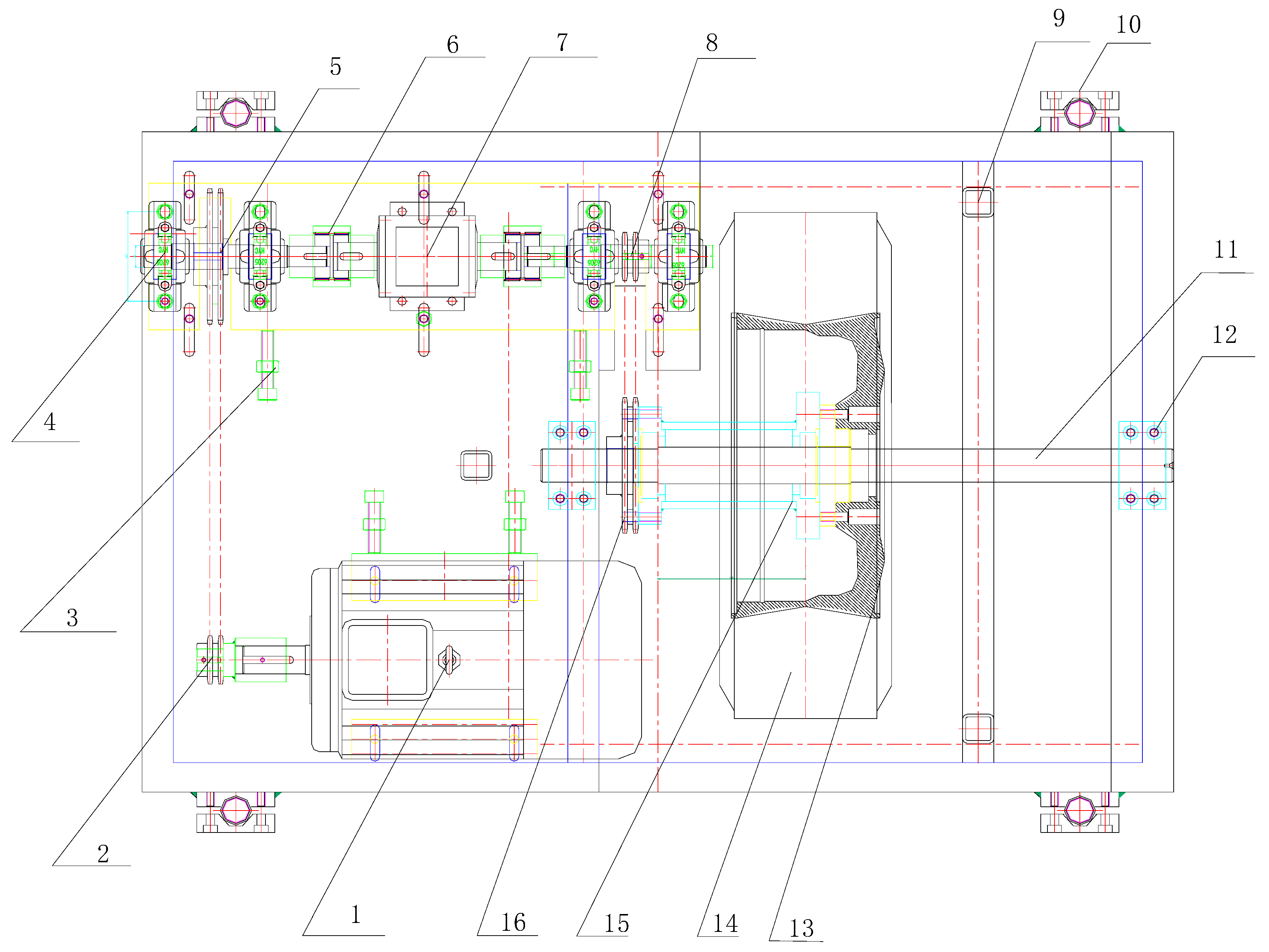
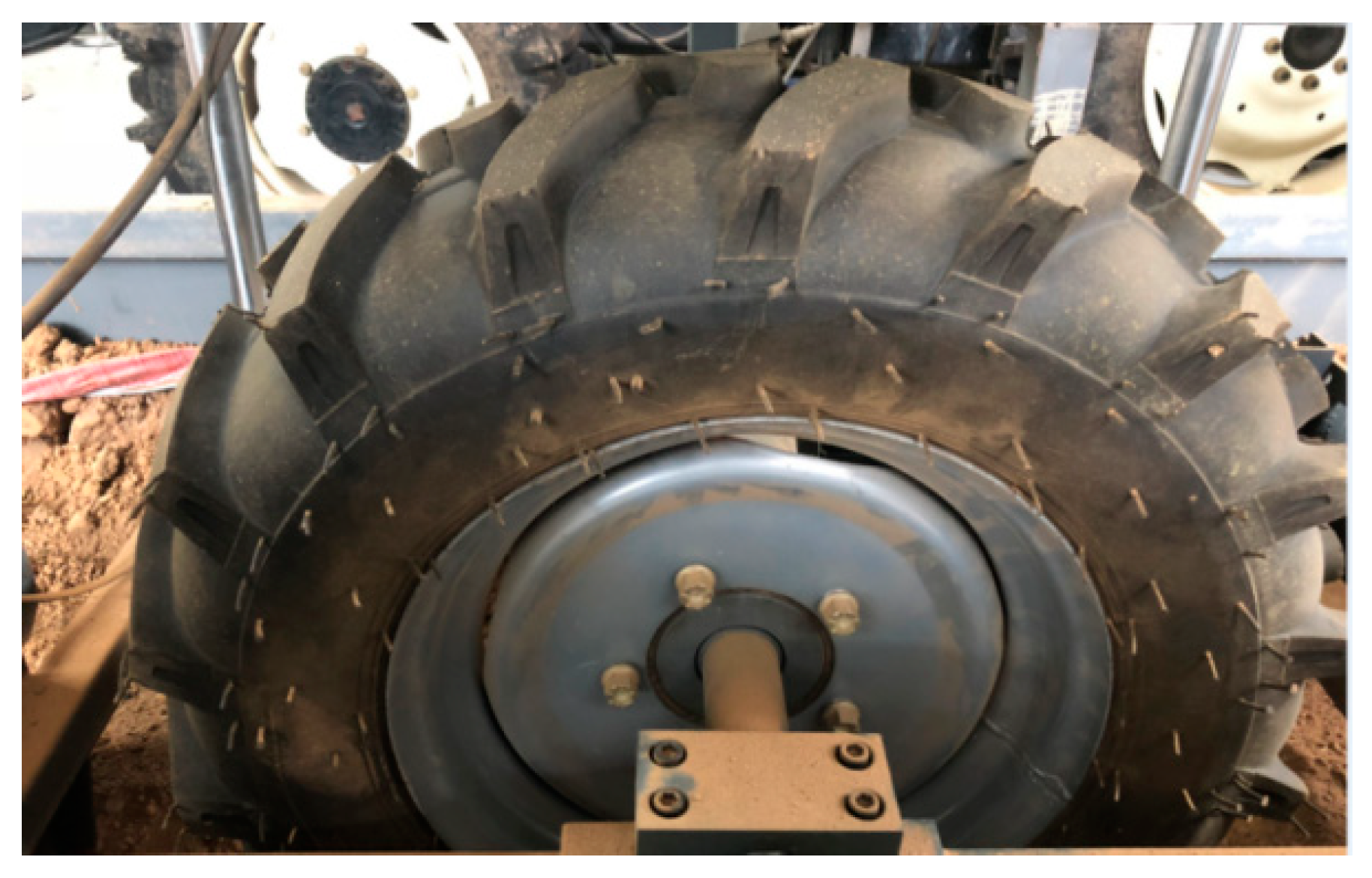
2.1.1. A Soil-Bin Testing Facility

The vehicle engineering laboratory of Nanjing Agriculture University developed the soil-bin testing facility (Figure 1) which was used for the experiments. The soil-bin was filled with sandy loam soil, and the size was 9 m × 1.5 m × 0.8 m (length × width × depth). The measured soil properties are listed in

Table 1. Mean soil physical properties.

Depth (cm)	Mean Dry Bulk Density (g/cm3)	Mean Soil Moisture Content (Wet Basis) w (%)	Soil Mechanical Composition/%			Mean Soil Compactness (kPa)
						Depth
			<0.002 mm	0.002–0.5 mm	>0.5 mm	100 mm	200 mm	300 mm
0–5	1.29	17.65	21.67	35.89	42.44	21	177	414

.

A 7.5 kW three-phase electric motor (model YVF132M-4; Nanjing Zhongke Co., Nanjing, China) was applied to supply tire input torque. The power is transferred to the wheel after two-stage deceleration and drives the tire rotation. To ensure the stability of the torque transmission, some adjusting bolts were installed near each bearing bracket and motor stand to adjust the tightness of the chain. A torque and rotational speed sensor was installed between the first brake sprocket and the second drive sprocket to measure the value of the torque and speed. In order to measure the 3D tractor tire contact area, it is necessary for the whole tire platform to move up and down in real-time in the process of driving and then describe the real deformation of the soil. Therefore, four vertical guide bars were installed at the four corners of the platform, and four springs were installed on the vertical guide rail, so that the platform moved smoothly up and down without beating. In addition, the platform was equipped with a triangular counterweight mounting plate through the counterweight plate support, which is convenient to analyze wheel-earth action under different loads.

The experiment was conducted in a soil-bin testing facility to investigate the effect of the tire-soil interface on contact area under different conditions of the speed, tire load, and inflation pressure, and soil moisture content of 17.65%. The utilized tire was a 6.00-14 bias-ply (four-ply rating) tire with high lugs, and it was a new one. A 6.00-14 bias-ply tire is often used as the tractor’s front wheel under 50 horsepower. The width of the tire is 153 mm and the half-width contains 18 wheel spikes. For the tire, the recommended inflation pressure of 180 kPa corresponds to the maximum capacity of 3.70 kN (China, 2017). In order to investigate the variation of the contact area under different values of inflation pressure (overinflated, slightly underinflated, and seriously underinflated), 207 kPa (overinflated), 138 kPa (slightly underinflated), and 69 kPa (seriously underinflated) tire pressures were selected in this paper. According to a maximum capacity of 3.7 kN and the maximum speed of the tire in the soil-bin, we chose the level of the tire load and the speed. Figure 2 shows the test tire, and

Table 2. Summary of examined parameters.

Level	Factor
	Tire Load (kN)	Inflation Pressure (kPa) 1	Speed (m/s)
1	1.5	207 (slightly overinflated)	1
2	2	138 (slightly underinflated)	2
3	2.5	69 (seriously underinflated)	3

¹ All tire loads used in this study were less than 3.70 kN so that we could investigate the effect of lower inflation pressures.

shows the influence factors and their corresponding value.

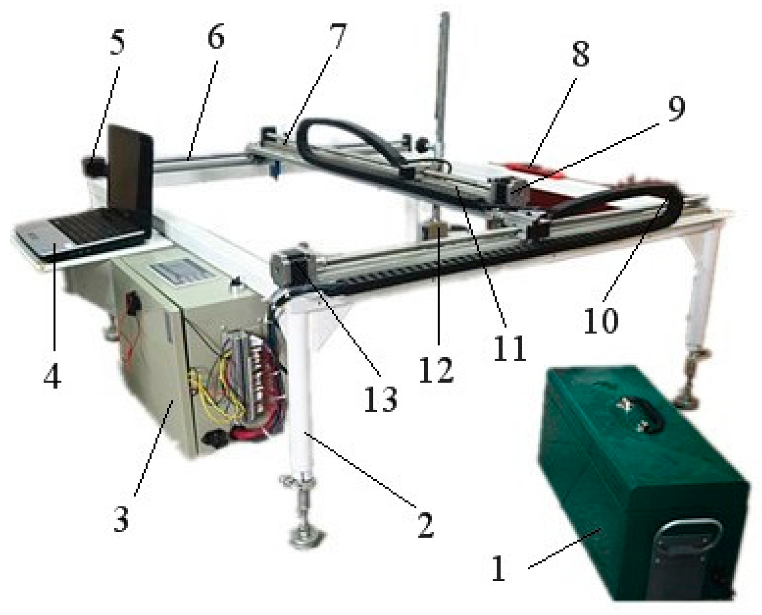
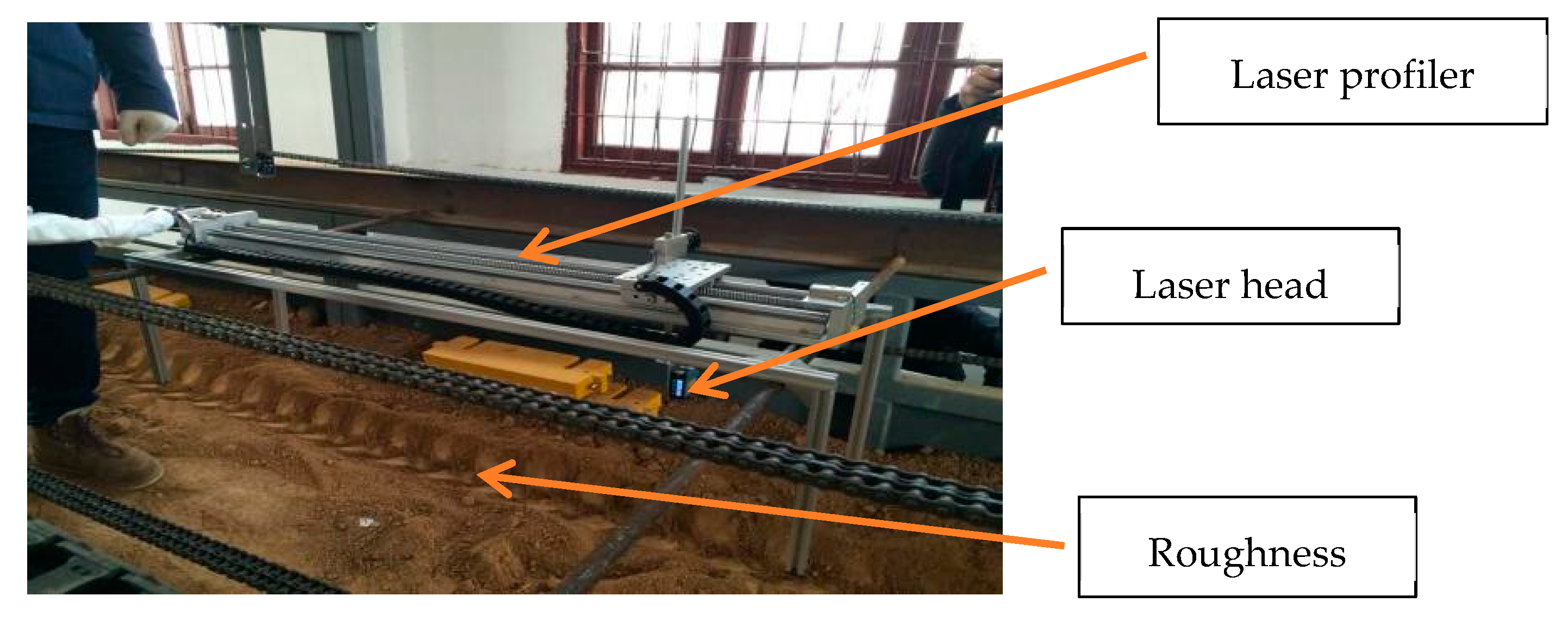
2.1.2. Laser Profiler

A laser profiler [24], independently manufactured by the Nanjing Agriculture University, was used to measure the roughness after rutting of the soil surface. A laser head, SICK DT20-P214B, was certified by CE, and the scanned area was 1 m × 1 m. The precision of the laser profiler is within ±0.5 mm, and the sampling interval was 5 mm.

The structure diagram is shown in Figure 3. The principle of the laser profiler is to measure the vertical distance between the standard and ground surface based on the triangulation technique. The real-time vertical distances were displayed in a software program in LabVIEW 2015 (v1.1). All these vertical distances formed the roughness curve of the ground surface.

Considering the size between the laser profiler and soil-bin, we took down the ball wire pair and servo motor of the laser profiler. Four support legs were used to support the laser profiler, and a gradienter was used to ensure the instrument’s level. The disassembled ball bars and control box were used to measure the soil roughness after rutting. Figure 4 shows the laser soil profile in use during the soil-bin experiments.

2.2. Experiment Method

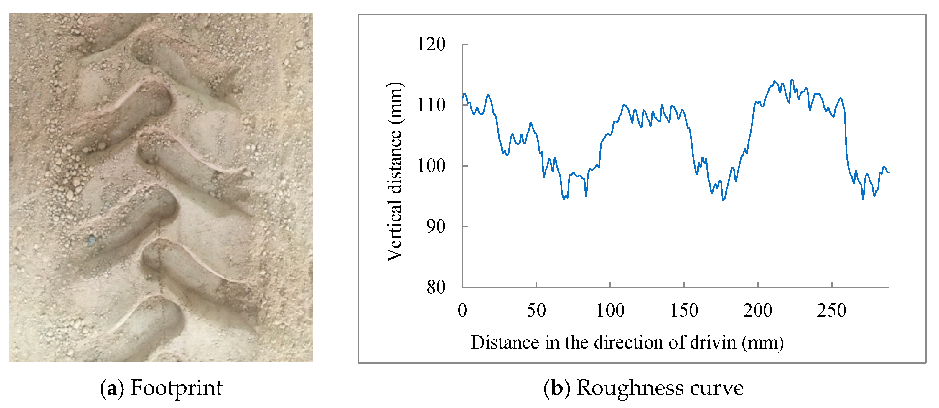
2.2.1. Roughness after Rutting

Since the width of the tire is 153 mm, and the sampling interval is 10 mm, 17 curves were measured to describe the roughness after rutting in each condition. These 17 curves made up the contact contour. To present the contact contour more exquisitely, we utilized the iterative function method for fractal interpolation. However, compared to the real roughness after rutting, the contact contour obtained by the laser profiler was upside-down. In this experiment, the measurement basic was 500 mm below the leaser head, and the test data minus 500 became the final data. All these data formed the real roughness after rutting. The roughness after rutting at a given speed (2 m/s), inflation pressure (207 kPa), and tire load (1.5 kN) is shown in Figure 5.

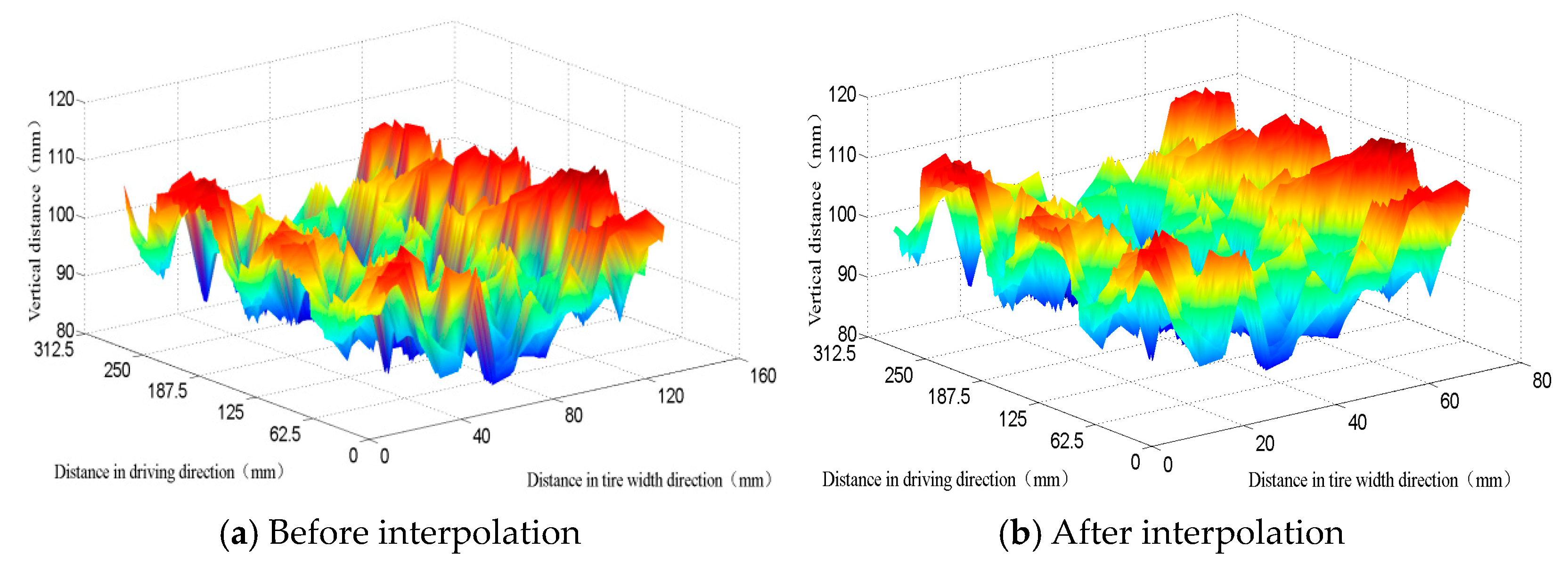
2.2.2. Fractal Interpolation Theory

The random 3D fractal interpolation theory [25] was used to interpolate the original measurement data. The initial point p₀ can be chosen at random, $p_0=p_i$, $p_i\in \{p_1, p_2, \cdots ,p_n\}$, and the data sequence is $x_1<x_2<\cdots <x_n$. The first point of iteration depends on p₀ and any set of affine functions, the second point of iteration depends on the first point and any set of affine functions, and so on, until the generated iteration point meets the requirements of subsequent finite element and simulation analysis. For example, if we chose $p_0=p_1=\left(x_1, y_1\right)$ as the initial point, the iterative process can be described as:

$$\begin{gathered} \widehat{p_1}\in \{F_{2,2}\left(p_0\right), F_{2,3}\left(p_0\right), F_{3,2}\left(p_0\right), F_{3,3}\left(p_0\right), \cdots , F_{N,M}\left(p_0\right)\} \\ \widehat{p_2}\in \{F_{2,2}\left(p_1\right), F_{2,3}\left(p_1\right), F_{3,2}\left(p_1\right), F_{3,3}\left(p_1\right), \cdots , F_{N,M}\left(p_1\right)\} \\ ⋮ \\ \widehat{p_n}\in \{F_{2,2}\left(p_{n-1}\right), F_{2,3}\left(p_{n-1}\right), F_{3,2}\left(p_{n-1}\right), F_{3,3}\left(p_{n-1}\right), \cdots , F_{N,M}\left(p_{n-1}\right)\} \end{gathered}$$

(1)

where $\widehat{p_n} \left(n=1, 2, 3, \cdots \right)$ is the basic interpolation data point, and F_N,M (N = 2, 3, …, N, M = 1, 2, …, M) is the test point.

If N′ is the total number of iterations, then the point set $\left\{(x_n, y_n|n=1, 2, \cdots , {\mathrm{N}}^{\prime }\right\}$ is all the reconstructed data points.

2.2.3. Roentgen Formula to Calculate the 3D Contact Area

The data collected by laser profiler is made up of matrix points and these points are distributed in three dimensions. Four adjacent non-coplanar points formed a small grid (Figure 6). And the mesh function is used to contact these small grids to form an intuitive 3D diagram. The total contact area equals the sum of all the small grid areas.

The small grid can be divided into two triangles, and the area of the grid is equal to the sum of the areas of the two triangles. The distance between AB, BC, CD, AD, and AC can be calculated by the distance formula between two points in space. According to Roentgen Formula, if the length of the three sides of the triangle are known, we can calculate the area of the triangle.

The Roentgen Formula is as follows:

$$A=\sqrt{l\left(l-a\right)\left(l-b\right)\left(l-c\right)}$$

(2)

$$l=\frac{a+b+c}{2}$$

(3)

where A is the area of the small grid formed by four adjacent non-coplanar points, and a, b, and c are the length of any two adjacent non-coplanar points.

The area of a quadrilateral formed by any four points:

$$A_{\mathrm{A}\mathrm{B}\mathrm{C}\mathrm{D}}=A_{\mathrm{A}\mathrm{B}\mathrm{C}}+A_{\mathrm{A}\mathrm{C}\mathrm{D}}$$

(4)

where A_ABCD is the area of any quadrilateral in space, A_ABC is the area of ΔABC, and A_ACD is the area of ΔACD.

2.2.4. Multiple Linear Regression

The contact area is influenced by the speed, tire load, and inflation pressure. Therefore, a functional relationship was proposed as the following type:

$$A=f\left(S,p,W\right)$$

(5)

where A is contact area, S is speed, p is inflation pressure, and W is tire load. We considered a full quadratic response for the vertical stress as follows:

$$A=a_0+a_1{x}_1+a_2{x}_2+a_3{x}_3+a_{11}{x}_1^2+a_{22}{x}_2^2+a_{33}{x}_3^2+a_{12}{x}_1{x}_2+a_{13}{x}_1{x}_3+a_{23}{x}_2{x}_3$$

(6)

where a₀, a₁, a₂, a₃, a₁₁, a₂₂, a₃₃, a₁₂, a₁₃, and a₂₃ are regression coefficients, x₁ is coded speed, x₂ is coded inflation pressure, x₃ is coded tire load, $\overline{S}$ is mean speed, S_max is maximum speed, S_min is minimum speed, $\overline{p}$ is mean inflation pressure, p_max is maximum inflation pressure, p_min is minimum inflation pressure, $\overline{W}$ is mean tire load, W_max is maximum tire load and W_min is minimum tire load.

Where $x_1=\frac{S-\overline{S}}{\left(S_{\max }-S_{\min }\right)/2}$, $x_2=\frac{p-\overline{p}}{\left(p_{\max }-p_{\min }\right)/2}$, $x_3=\frac{W-\overline{W}}{\left(W_{\max }-W_{\min }\right)/2}$, $\overline{S}$ = 2 m/s, $S_{\max }$ = 3 m/s, $S_{\min }$= 1 m/s, $\overline{p}$ = 138 kPa, $p_{\max }$ = 207 kPa, $p_{\min }$ = 69 kPa, $\overline{W}$ = 2 kN, $W_{\max }$ = 2.5 kN, and $W_{\min }$ = 1.5 kN.

Therefore:

$$x_1=\frac{S-\overline{S}}{\left(S_{\max }-S_{\min }\right)/2}=S-2$$

(7)

$$x_2=\frac{p-\overline{p}}{\left(p_{\max }-p_{\min }\right)/2}=\frac{p-138}{69}$$

(8)

$$x_3=\frac{W-\overline{W}}{\left(W_{\max }-W_{\min }\right)/2}=2W-4$$

(9)

Table 3. Parameters and the coded result of S, p, and W.

Parameters			Coded Values
S (m/s)	p (kPa)	W (kN)	x1	x2	x3
1	69	1.5	−1	−1	−1
2	138	2	0	0	0
3	207	2.5	1	1	1

presents the levels and coded values of the independent variables (S, p, and W). In this study, we analyze the coded data based on a backward variable selection technique in SAS (SAS Institute, Cary, NC, USA), and the resulting regression equation only focused on the significant variables.

3. Results and Discussion

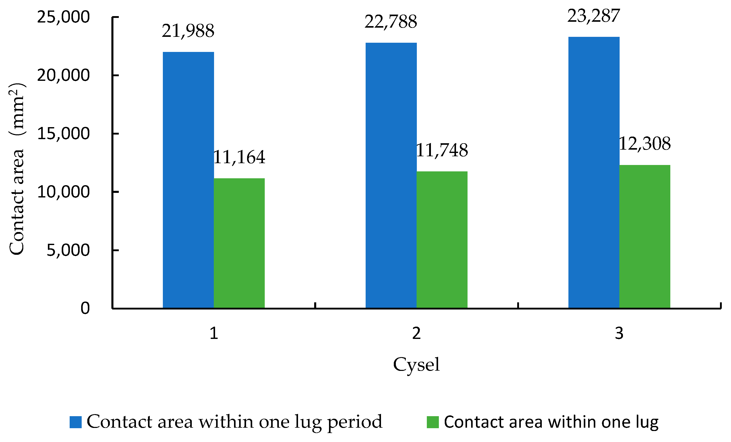
3.1. The Distribution Rule of Contact Area under the Same Tire Pattern Cycle

Theoretically, a tire with a chevron tread pattern is periodic, and the contact area of the ground surface is also periodic. However, the complexity of soil characteristics influences the contact area’s periodicity. In this paper, we chose one set of experiments to study the contact area’s periodicity at a given speed, inflation pressure, and tire load (S = 2 m/s, p = 69 kPa, and W = 1.5 kN). Figure 7 shows a 3D curve of tire contact patterns within three lug cycles. In Figure 8, the contact width is 139 mm, and the contact length is 290 mm, while the single contact lengths are 96.25 mm, 97.5 mm, and 96.25 mm, respectively. Figure 8 shows the contact area of a single cycle and the contact area of a single-wheel spur.

As shown in Figure 8, the contact area of the tire still has periodicity, and the contact area within a single cycle changed little at a given condition, indicating that the soil characteristics in the soil-bin were almost the same. At the same time, the width of the chevron tread pattern in the tire was obviously less than the width of the tread, but the contact area of a single chevron tread pattern was more than half of the contact area within a cycle. That was to say, the contact area of a chevron tread pattern was slightly larger than the area of the tread because of the height of the chevron tread pattern.

3.2. Fractal Dimension

Figure 9 shows the comparison of contact area between the graphical before and after interpolation (p = 69 kPa, W = 1.5 kN, and S = 2 m/s). Based on the Iterative function system and Fractal interpolation theory, the fractal dimensions of the contact surface before and after interpolation were 2.20 and 2.27, respectively, and the non-scale range is the same. The similar correlation coefficient indicated that the surface became smoother, but the structure was not changed. The actual contact width was 138 mm.

3.3. Empirical Equation for Contact Area

The significant variables from the results of the statistical analysis of the contact area and the influence factors based on the backward analysis technique in SAS are listed in

Table 4. Main influence factors for contact area.

Variable	Parameter Estimate	Standard Error	Pr Value
Intercept	68,525	13,213	<0.0001
x1	596	3.33	0.083
x2	−3220	97	<0.0001
x3	1865	33	<0.0001
x12	−1270	5	0.0362
x22	−1880	11	0.0034
x2x3	1568	15	0.0008

.

The resulting regression equation is:

$$A=a_0+a_1{x}_1+a_2{x}_2+a_3{x}_3+a_{11}{x}_1^2+a_{22}{x}_2^2+a_{23}{x}_2{x}_3$$

(10)

Because x₁, x₂, and x₃ are given by Equation (7) through (9), Equation (10) can be written as:

$$A=\mathrm{68,525}+596(S-2)-3220\left(\frac{p-138}{69}\right)+3730\left(W-2\right)-1270{\left(S-2\right)}^2-1880{\left(\frac{p-138}{69}\right)}^2+3136\left(\frac{p-138}{69}\right)\left(W-2\right)$$

(11)

Equation (11) is a comprehensive equation that incorporates the effect of speed, inflation pressure and vertical load on the contact area between the soil and tire. It contains 10 empirical coefficients, of which only 6 are significant. It has an R² value of 90.80%, which means this prediction equation has a high predictive ability. And all the variables included in the study were equidistant to ensure no multicollinearity issues in model selection. Therefore, the prediction equation is robust to the coefficients. This equation shows that the contact area increased with the increase in speed and tire load while it decreased with the increase in inflation pressure. Of the model parameters, inflation pressure had the greatest influence on vertical stress, followed by tire load and speed. And the prediction equation can be used to preliminary estimate the soil compaction, which directly affects the sustainability of agriculture [2,8].

Equation (11) provides further insight into the influence of speed, inflation pressure, and tire load on the contact area. For a given inflation pressure and tire load (p = 138 kPa and W = 2 kN), Equation (8) reduces to:

$$A=\mathrm{68,525}+596(S-2)-1270{\left(S-2\right)}^2$$

(12)

Equation (12) means that the contact area at a given inflation pressure and tire load varies in a quadratic manner with the speed (Figure 10a). Alternatively, at a given speed and tire load (S = 2 m/s and W = 2 kN), we obtain the following equation:

$$A=\mathrm{68,525}-3220\left(\frac{p-138}{69}\right)-1880{\left(\frac{p-138}{69}\right)}^2$$

(13)

Equation (13) means that the contact area at a given speed and tire load varies in a quadratic manner with the inflation pressure (Figure 10b). In addition, at a given speed and inflation pressure (S = 2 m/s and p = 138 kPa), Equation (11) becomes:

$$A=\mathrm{68,525}+3730\left(W-2\right)$$

(14)

Equation (14) means that the contact area is linearly related to the tire load at a given speed and inflation pressure, as shown in Figure 10c.

3.4. Combination Influence of Influence Factors

The combination influence of speed, inflation pressure, and tire load is shown in Figure 11.

As shown in Figure 11, the contact area increased as the tire load increased, while the contact area decreased as the inflation pressure increased [26]. This is because the high tire load increased the contact width, while the high inflation pressure decreased the contact length and width. When the inflation pressure was 69 kPa or 138 kPa, the contact area was changed minorly. When the inflation pressure was 207 kPa, and the tire load increased from 1.5 kN and 2 kN to 2.5 kN, the contact area had changed greatly. This is because the high inflation pressure decreased the contact length and width, but increased the contact depth, while the low tire load decreased the contact depth. So, the combination of high speed, high inflation pressure, and low tire load (S = 3 m/s, p = 207 kPa, and W = 1.5 kN) led to the smallest contact area (A = 59,019 mm²), while the combination of high speed, low inflation pressure, and high tire load (S = 3 m/s, p = 69 kPa, and W = 2.5 kN) led to the biggest contact area [27] (A = 69,934 mm²), which also led the biggest soil compaction and is not conducive to the sustainable development of agriculture.

4. Conclusions

In this study, we investigated the effects of speed, inflation pressure, and tire load on the contact area between the tire and the soil in the signal tire soil-bin. We reached the following conclusions:

• The width of a chevron tread pattern in the tire was obviously less than the width of the tread, but the contact area of a single chevron tread pattern was more than half of the contact area within a cycle. That was to say, the contact area of a chevron tread pattern was slightly larger than the area of the tread because of the height of the chevron tread pattern.
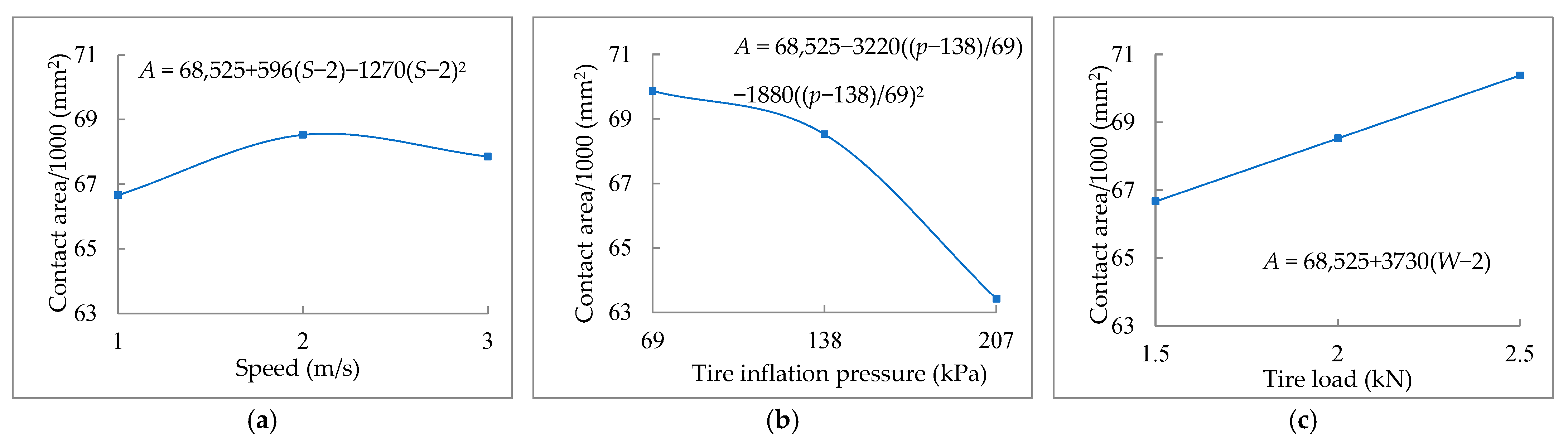
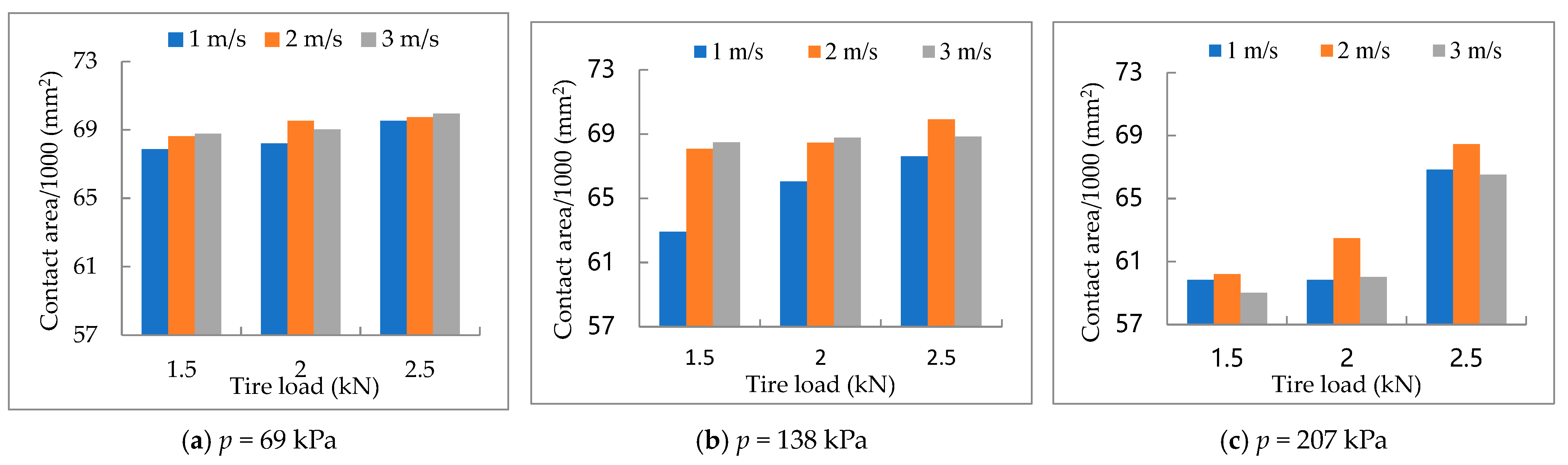
• The empirical Equations (12)–(14) demonstrated that the contact area varied in a quadratic manner with speed at a given inflation pressure and tire load and varied in a quadratic manner with inflation pressure at a given speed and tire load and varied linearly with the tire load for a given speed and inflation pressure.
• The combination of high speed (S = 3 m/s), low inflation pressure (69 kPa), and high tire load (W = 2.5 kN) led to the biggest contact area (A = 69,934 mm²) and possibly severe soil compact and unsustainable development of agriculture. Therefore, this combination of speed, inflation pressure, and tire load is not recommended for the soil conditions used in this study.

References

1. Teimourlou, R.F.; Taghavifar, H. Determination of the Super-Elliptic Shape of Tire-Soil Contact Area Using Image Processing Method. Cercet. Agron. Mold. 2015, 48, 5–14. [Google Scholar] [CrossRef]
2. Kokieva, E.G.; Troyanovskaya, I.P.; Orekhovskaya, A.A.; Kalimullin, M.N.; Dzjasheev, A.-M.S.; A Ivanov, A.; A Sokolova, V. Research of soil compaction process in area of contact with a wheel mover. J. Phys. Conf. Ser. 2021, 2094, 042003. [Google Scholar] [CrossRef]
3. Lu, J.; Cheng, M.; Zhao, C.; Li, B.; Peng, H.; Zhang, Y.; Shao, Q.; Hassan, M. Application of lignin in preparation of slow-release fertilizer: Current status and future perspectives. Ind. Crops Prod. 2021, 176, 114267. [Google Scholar] [CrossRef]
4. Yue, K.; Fornara, D.A.; Heděnec, P.; Wu, Q.; Peng, Y.; Peng, X.; Ni, X.; Wu, F.; Peñuelas, J. No tillage decreases GHG emissions with no crop yield tradeoff at the global scale. Soil Tillage Res. 2023, 228, 105643. [Google Scholar] [CrossRef]
5. Memon, M.S.; Guo, J.; Tagar, A.A.; Perveen, N.; Ji, C.; Memon, S.A.; Memon, N. The effects of tillage and straw incorporation on soil organic carbon status, rice crop productivity, and sustainability in the rice-wheat cropping system of eastern China. Sustainability 2018, 10, 961. [Google Scholar] [CrossRef] [Green Version]
6. Farhadi, P.; Golmohammadi, A.; Malvajerdi, A.S.; Shahgholi, G. Finite element modeling of the interaction of a treaded tire with clay-loam soil. Comput. Electron. Agric. 2019, 162, 793–806. [Google Scholar] [CrossRef]
7. Batey, T. Soil compaction and soil management—A review. Soil Use Manag. 2009, 25, 335–345. [Google Scholar] [CrossRef]
8. Júnnyor, W.D.S.G.; Diserens, E.; De Maria, I.C.; Araujo-Junior, C.F.; Farhate, C.V.V.; de Souza, Z.M. Prediction of soil stresses and compaction due to agricultural machines in sugarcane cultivation systems with and without crop rotation. Sci. Total Environ. 2019, 681, 424–434. [Google Scholar] [CrossRef]
9. Augustin, K.; Kuhwald, M.; Brunotte, J.; Duttmann, R. Wheel Load and Wheel Pass Frequency as Indicators for Soil Compaction Risk: A Four-Year Analysis of Traffic Intensity at Field Scale. Geosciences 2020, 10, 292. [Google Scholar] [CrossRef]
10. Wulfsohn, D. Soil-Tire Contact area. In Advances in Soil Dynamics; Upadhyaya, S.K., Chancellor, W.J., Perumpral, J.V., Wulfsohn, D., Way, T.R., Eds.; American Society of Agricultural and Biological Engineers: St. Joseph, MI, USA, 2009; Volume 3, p. 59. [Google Scholar]
11. Wong, J. Theory of Ground Vehicles; John Wiley & Sons Inc.: Hoboken, NJ, USA, 2021. [Google Scholar] [CrossRef]
12. Upadhyaya, S.; Wolf, D.; Chancellor, W.J.; Shmulevich, I.; Hadas, A. Traction-Soil Compaction Tradeoffs as a Function of Dynamic Soil-Tire Interation Due to Varying Soil and Loading Conditions; United States Department of Agriculture: Washington, DC, USA, 1995. [Google Scholar] [CrossRef]
13. Grečenko, A. Tyre footprint area on hard ground computed from catalogue values. J. Terramech. 1995, 32, 325–333. [Google Scholar] [CrossRef]
14. Schjønning, P.; Lamandé, M.; Tøgersen, F.A.; Arvidsson, J.; Keller, T. Modelling effects of tyre inflation pressure on the stress distribution near the soil–tyre interface. Biosyst. Eng. 2007, 99, 119–133. [Google Scholar] [CrossRef]
15. Arvidsson, J.; Keller, T. Soil stress as affected by wheel load and tyre inflation pressure. Soil Tillage Res. 2007, 96, 284–291. [Google Scholar] [CrossRef]
16. Diserens, E. Calculating the contact area of trailer tyres in the field. Soil Tillage Res. 2009, 103, 302–309. [Google Scholar] [CrossRef]
17. Zhang, J.; Kong, X.; Obrien, E.J.; Peng, J.; Deng, L. Noncontact measurement of tire deformation based on computer vision and Tire-Net semantic segmentation. Measurement 2023, 217, 113034. [Google Scholar] [CrossRef]
18. Taghavifar, H.; Mardani, A. Potential of functional image processing technique for the measurements of contact area and contact pressure of a radial ply tire in a soil bin testing facility. Measurement 2013, 46, 4038–4044. [Google Scholar] [CrossRef]
19. Cueto, O.G.; Coronel, C.E.I.; Bravo, E.L.; Morfa, C.A.R.; Suárez, M.H. Modelling in FEM the soil pressures distribution caused by a tyre on a Rhodic Ferralsol soil. J. Terramech. 2016, 63, 61–67. [Google Scholar] [CrossRef]
20. Michael, M.; Vogel, F.; Peters, B. DEM–FEM coupling simulations of the interactions between a tire tread and granular terrain. Comput. Methods Appl. Mech. Eng. 2015, 289, 227–248. [Google Scholar] [CrossRef]
21. Botta, G.; Becerra, A.T.; Tourn, F.B. Effect of the number of tractor passes on soil rut depth and compaction in two tillage regimes. Soil Tillage Res. 2009, 103, 381–386. [Google Scholar] [CrossRef]
22. Kenarsari, A.E.; Vitton, S.J.; Beard, J.E. Creating 3D models of tractor tire footprints using close-range digital photogrammetry. J. Terramech. 2017, 74, 1–11. [Google Scholar] [CrossRef]
23. Farhadi, P.; Golmohammadi, A.; Sharifi, A.; Shahgholi, G. Potential of three-dimensional footprint mold in investigating the effect of tractor tire contact volume changes on rolling resistance. J. Terramech. 2018, 78, 63–72. [Google Scholar] [CrossRef]
24. Jiang, C.; Lu, Z.; Upadhyaya, S.K.; Memon, M.S. Measurement and Analysis of the Vertical Stress Distribution within a Cultivated Soil Volume under Static Conditions. Trans. ASABE 2019, 62, 1035–1043. [Google Scholar] [CrossRef]
25. Barnsley, M.F. Fractal functions and interpolation. Constr. Approx. 1986, 2, 32–303. [Google Scholar] [CrossRef]
26. Yadav, R.; Raheman, H. Development of an artificial neural network model with graphical user interface for predicting contact area of bias-ply tractor tyres on firm surface. J. Terramech. 2023, 107, 1–11. [Google Scholar] [CrossRef]
27. Ptak, W.; Czarnecki, J.; Brennensthul, M.; Lejman, K.; Małecka, A. Evaluation of Tire Footprint in Soil Using an Innovative 3D Scanning Method. Agriculture 2023, 13, 514. [Google Scholar] [CrossRef]
Figure 1. Soil-bin testing facility. 1. Driving motor; 2. The first drive sprocket; 3. Adjusting bolt; 4. Bearing pedestal; 5. The first brake sprocket; 6. Shaft coupling; 7. Torque transducer; 8. The second drive sprocket; 9. Counterweight plate bearing; 10. Vertical guide bearing; 11. The wheel fixed shaft; 12. Axle fixed support; 13. Wheel; 14. Tire; 15. Hub; 16. The second brake sprocket.
Sustainability 15 10017 g001
Figure 2. Test tire.
Sustainability 15 10017 g002
Figure 3. Laser profiler. 1. servo motor (x-direction); 2. cable carrier for surrounding and guiding the flexible cables; 3. laser sensor; 4. servo motor (y-direction); 5, 13. control box; 6. electric power; 7, 11. ruler with a level; 8. trundle with moving horizontal beam to which laser sensor is mounted; 9. ball screw pair with double optical axis; 10. tank chain; 12. laser head.
Sustainability 15 10017 g003
Figure 4. Measurement of roughness by laser profiler.
Sustainability 15 10017 g004
Figure 5. Roughness after rutting.
Sustainability 15 10017 g005
Figure 6. Random four points in space.
Sustainability 15 10017 g006
Figure 7. A 3D curve of tire contact pattern within three lug cycles.
Sustainability 15 10017 g007
Figure 8. The contact area of single lug period within the wheel-soil contact area.
Sustainability 15 10017 g008
Figure 9. Comparison of contact area between the graphical before and after interpolation (p = 69 kPa, W = 1.5 kN, and S = 2 m/s).
Sustainability 15 10017 g009
Figure 10. Equation (11) provides insight into the influence of the speed, inflation pressure, and tire load: (a) relationship between contact area and speed, when p = 138 kPa and W = 2 kN; (b) relationship between contact area and inflation pressure, when S = 2 m/s and W = 2 kN; and (c) relationship between contact area and tire load, when S = 2 m/s and p = 138 kPa.
Sustainability 15 10017 g010
Figure 11. Influence of speed, inflation pressure, and tire load on contact area.
Sustainability 15 10017 g011