


On Employing a Constrained Nonlinear Optimizer to Constrained Economic Dispatch Problems

 ,
,  ,
,  ,
,
Abstract
:1. Introduction
1.1. Background
1.2. Literature Review
1.3. Contribution
1.4. Paper Organization
2. ELD Problem Formulation
3. Interior Point Algorithm
3.1. Original Problem
3.2. Approximate Problem
3.3. Barrier Function
3.4. Lagrangian Function
3.5. KKT Conditions
3.6. Solution to KKT System
3.6.1. Newton or Direct Step
3.6.2. Conjugate Gradient (CG) Step
3.7. Next Iteration and Step Size
3.8. Merit Function
3.9. Updating Barrier Parameter
3.9.1. Monotonically
3.9.2. By Predictor–Corrector
| Algorithm 1. Primal–dual interior–point algorithm | |
| 1: | Initialize and Lagrangian multipliers . |
| 2: | Choose threshold parameter , parameter , trust-region radius , barrier parameter and . |
| 3: | Set . |
| 4: | Define and . |
| 5: | Repeat until an original nonlinear stopping test is met: |
| 6: | Repeat until KKT conditions are met: |
| 7: | Factor the primal-dual system and count its coefficient matrix’s negative eigenvalues nEig. |
| 8: | Set LineSearch = False, |
| 9: | If nEig , |
| 10: | Obtain the search direction . |
| 11: | Compute , . |
| 12: | If , |
| 13: | Update the penalty parameter . |
| 14: | Compute a steplength such that |
| 15: | |
| 16: | If |
| 17: | Set |
| 18: | Set . |
| 19: | Set LineSearch = True. |
| 20: | Endif |
| 21: | Endif |
| 22: | Endif |
| 23: | If LineSearch = False, |
| 24: | Compute |
| 25: | Endif |
| 26: | Compute . |
| 27: | Set . |
| 28: | Set . |
| 29: | End |
| 30: | Reduce barrier parameter µ monotonically or by “predictor–corrector.” |
| 31: | End |
4. Simulation Results
4.1. Case Study 1: 3-Unit System
4.1.1. Without VPL Effects
4.1.2. With VPL Effects
4.2. Case Study 2: 10-Unit System
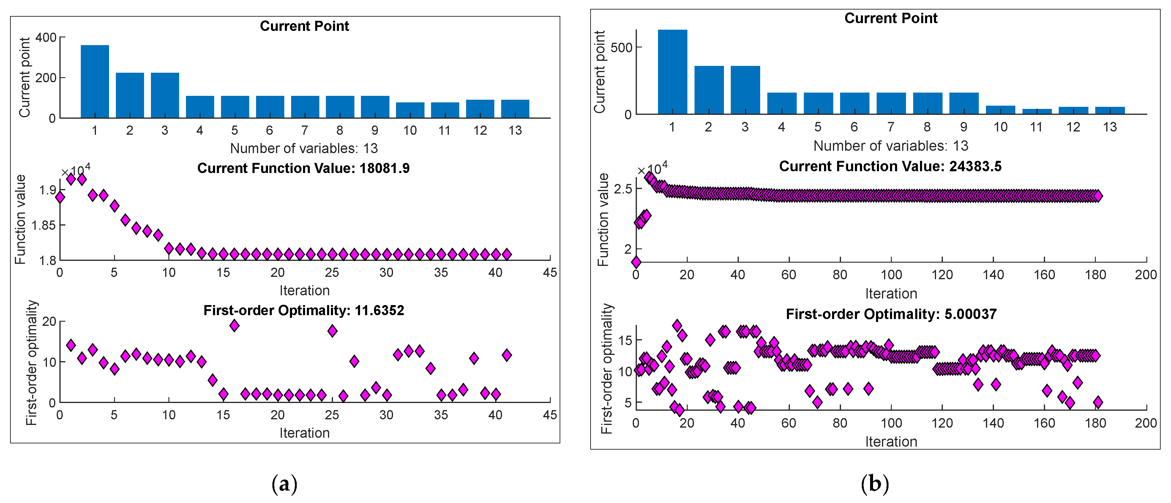
4.3. Case Study 3: 13-Unit System
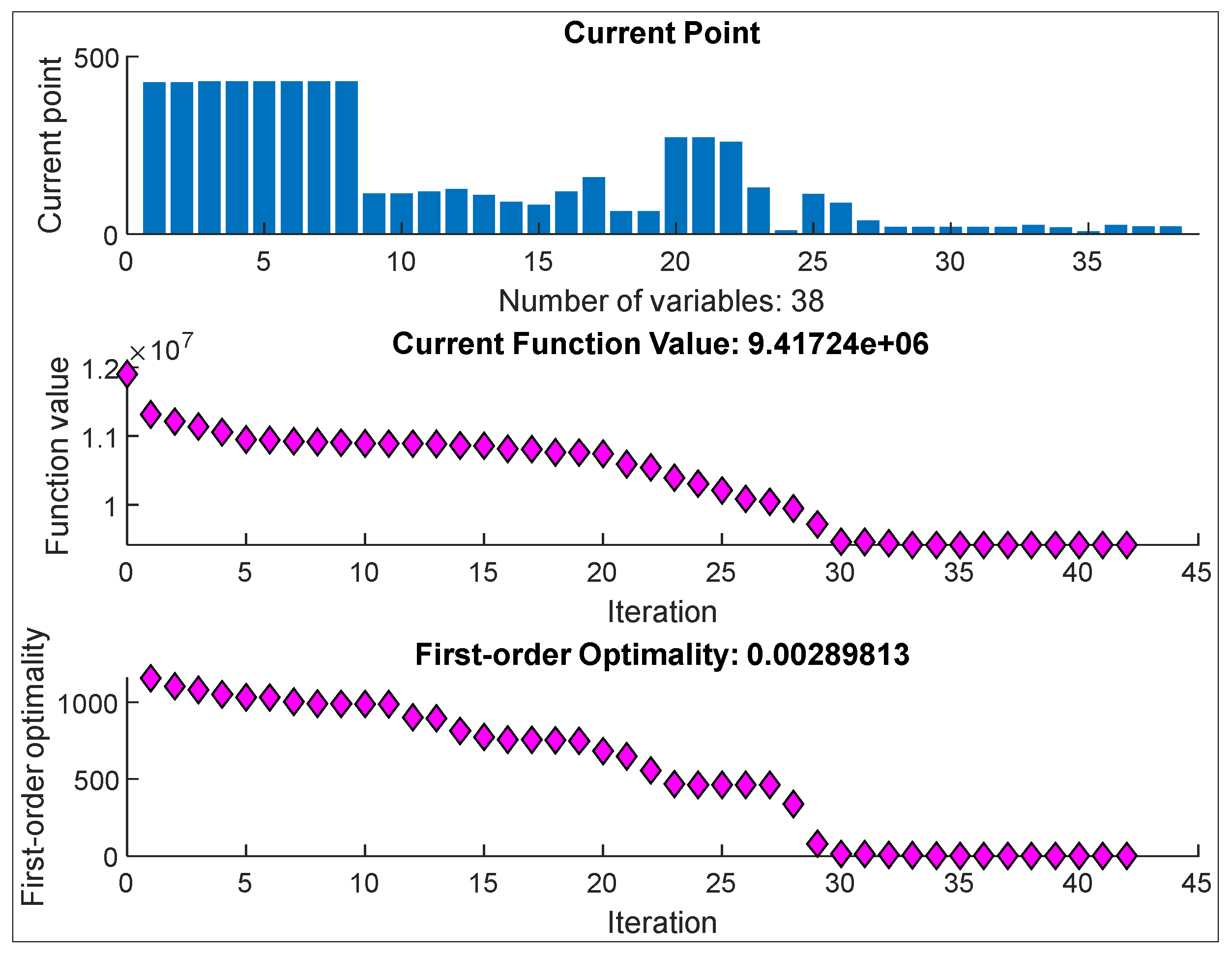
4.4. Case Study 4: 38-Unit System
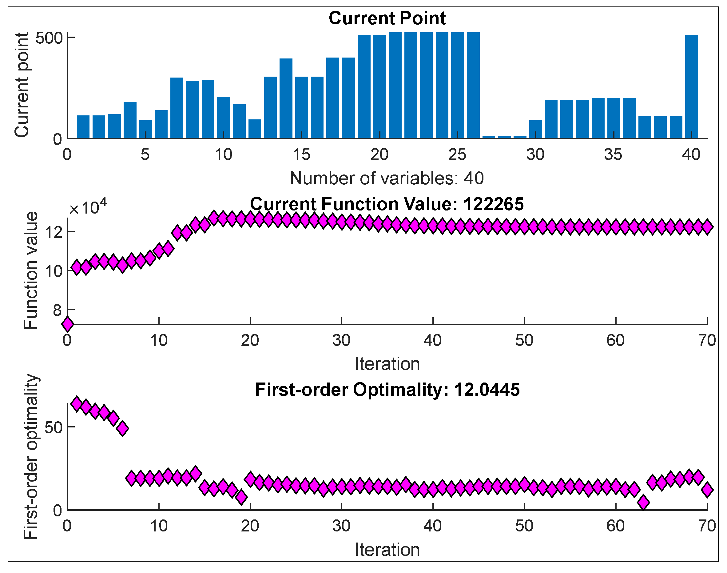
4.5. Case Study 5: 40-Unit System
5. Conclusions
Author Contributions
Funding
Institutional Review Board Statement
Informed Consent Statement
Data Availability Statement
Acknowledgments
Conflicts of Interest
References
- Iqbal, M.A.; Fakhar, M.S.; Ul Ain, N.; Tahir, A.; Khan, I.A.; Abbas, G.; Kashif, S.A.R. A New Fast Deterministic Economic Dispatch Method and Statistical Performance Evaluation for the Cascaded Short-Term Hydrothermal Scheduling Problem. Sustainability 2023, 15, 1644. [Google Scholar] [CrossRef]
- Khan, N.A.; Sidhu, G.A.S.; Gao, F. Optimizing Combined Emission Economic Dispatch for Solar Integrated Power Systems. IEEE Access 2016, 4, 3340–3348. [Google Scholar] [CrossRef]
- Csercsik, D.; Kádár, P. Performance Analysis of MATLAB Solvers in the Case of a Quadratic Programming Generation Scheduling Optimization Problem. Int. J. Energy Power Eng. 2019, 13, 8–12. [Google Scholar]
- Pinheiro, R.B.; Balbo, A.R.; Nepomuceno, L. Solving Network-Constrained Nonsmooth Economic Dispatch Problems through a Gradient-Based Approach. Int. J. Electr. Power Energy Syst. 2019, 113, 264–280. [Google Scholar] [CrossRef]
- Jabr, R.A.; Coonick, A.H.; Cory, B.J. A Homogeneous Linear Programming Algorithm for the Security Constrained Economic Dispatch Problem. IEEE Trans. Power Syst. 2000, 15, 930–936. [Google Scholar] [CrossRef]
- Nanda, J.; Hari, L.; Kothari, M.L. Economic Emission Load Dispatch with Line Flow Constraints Using a Classical Technique. IEE Proc. Gener. Transm. Distrib. 1994, 141, 1–10. [Google Scholar] [CrossRef]
- Chowdhury, B.H.; Rahman, S. A Review of Recent Advances in Economic Dispatch. IEEE Trans. Power Syst. 1990, 5, 1248–1259. [Google Scholar] [CrossRef]
- Granelli, G.P.; Marannino, P.; Montagna, M.; Silvestri, A. Fast and Efficient Gradient Projection Algorithm for Dynamic Generation Dispatching. IEE Proc. C Gener. Transm. Distrib. 1989, 136, 295–302. [Google Scholar] [CrossRef]
- Barcelo, W.R.; Rastgoufard, P. Dynamic Economic Dispatch Using the Extended Security Constrained Economic Dispatch Algorithm. IEEE Trans. Power Syst. 1997, 12, 961–967. [Google Scholar] [CrossRef]
- Liang, Z.-X.; Glover, J.D. A Zoom Feature for a Dynamic Programming Solution to Economic Dispatch Including Transmission Losses. IEEE Trans. Power Syst. 1992, 7, 544–550. [Google Scholar] [CrossRef]
- Shoults, R.R.; Chakravarty, R.K.; Lowther, R. Quasi-Static Economic Dispatch Using Dynamic Programming with an Improved Zoom Feature. Electr. Power Syst. Res. 1996, 39, 215–222. [Google Scholar] [CrossRef]
- Lee, F.N.; Breipohl, A.M. Reserve Constrained Economic Dispatch with Prohibited Operating Zones. IEEE Trans. Power Syst. 1993, 8, 246–254. [Google Scholar] [CrossRef]
- Fan, J.Y.; McDonald, J.D. A Practical Approach to Real Time Economic Dispatch Considering Unit’s Prohibited Operating Zones. IEEE Trans. Power Syst. 1994, 9, 1737–1743. [Google Scholar] [CrossRef]
- Goncalves, E.; Balbo, A.R.; da Silva, D.N.; Nepomuceno, L.; Baptista, E.C.; Soler, E.M. Deterministic Approach for Solving Multiobjective Nonsmooth Environmental and Economic Dispatch Problem. Int. J. Electr. Power Energy Syst. 2019, 104, 880–897. [Google Scholar] [CrossRef]
- Chen, J.; Zhang, Y. A Lagrange Relaxation-Based Alternating Iterative Algorithm for Nonconvex Combined Heat and Power Dispatch Problem. Electr. Power Syst. Res. 2019, 177, 105982. [Google Scholar] [CrossRef]
- Abbas, G.; Gu, J.; Farooq, U.; Asad, M.U.; El-Hawary, M. Solution of an Economic Dispatch Problem through Particle Swarm Optimization: A Detailed Survey—Part I. IEEE Access 2017, 5, 15105–15141. [Google Scholar] [CrossRef]
- Abbas, G.; Gu, J.; Farooq, U.; Raza, A.; Asad, M.U.; El-Hawary, M.E. Solution of an Economic Dispatch Problem through Particle Swarm Optimization: A Detailed Survey—Part II. IEEE Access 2017, 5, 24426–24445. [Google Scholar] [CrossRef]
- Tai, T.-C.; Lee, C.-C.; Kuo, C.-C. A Hybrid Grey Wolf Optimization Algorithm Using Robust Learning Mechanism for Large Scale Economic Load Dispatch with Vale-Point Effect. Appl. Sci. 2023, 13, 2727. [Google Scholar] [CrossRef]
- Pang, A.; Liang, H.; Lin, C.; Yao, L. A Surrogate-Assisted Adaptive Bat Algorithm for Large-Scale Economic Dispatch. Energies 2023, 16, 1011. [Google Scholar] [CrossRef]
- Al-Bahrani, L.; Seyedmahmoudian, M.; Horan, B.; Stojcevski, A. Solving the Real Power Limitations in the Dynamic Economic Dispatch of Large-Scale Thermal Power Units under the Effects of Valve-Point Loading and Ramp-Rate Limitations. Sustainability 2021, 13, 1274. [Google Scholar] [CrossRef]
- Sakthivel, V.P.; Suman, M.; Sathya, P.D. Squirrel Search Algorithm for Economic Dispatch with Valve-Point Effects and Multiple Fuels. Energy Sources Part B Econ. Plan. Policy 2020, 15, 351–382. [Google Scholar] [CrossRef]
- Ahmed, I.; Alvi, U.-E.-H.; Basit, A.; Khursheed, T.; Alvi, A.; Hong, K.-S.; Rehan, M. A Novel Hybrid Soft Computing Optimization Framework for Dynamic Economic Dispatch Problem of Complex Nonconvex Contiguous Constrained Machines. PLoS ONE 2022, 17, e0261709. [Google Scholar] [CrossRef]
- Ghasemi, M.; Akbari, E.; Zand, M.; Hadipour, M.; Ghavidel, S.; Li, L. An Efficient Modified HPSO-TVAC-Based Dynamic Economic Dispatch of Generating Units. Electr. Power Compon. Syst. 2019, 47, 1826–1840. [Google Scholar] [CrossRef]
- Nguyen, T.-T.; Wang, M.-J.; Pan, J.-S.; Dao, T.; Ngo, T.-G. A Load Economic Dispatch Based on Ion Motion Optimization Algorithm. In Advances in Intelligent Information Hiding and Multimedia Signal Processing, Proceedings of the 15th International Conference on IIH-MSP in Conjunction with the 12th International Conference on FITAT, Jilin, China, 18–20 July 2020; Springer: Berlin/Heidelberg, Germany, 2020; Volume 2, pp. 115–125. [Google Scholar]
- Singh, D.; Dhillon, J.S. Ameliorated Grey Wolf Optimization for Economic Load Dispatch Problem. Energy 2019, 169, 398–419. [Google Scholar] [CrossRef]
- Younes, Z.; Alhamrouni, I.; Mekhilef, S.; Reyasudin, M. A Memory-Based Gravitational Search Algorithm for Solving Economic Dispatch Problem in Micro-Grid. Ain Shams Eng. J. 2021, 12, 1985–1994. [Google Scholar] [CrossRef]
- Karimi, N.; Khandani, K. Social Optimization Algorithm with Application to Economic Dispatch Problem. Int. Trans. Electr. Energy Syst. 2020, 30, e12593. [Google Scholar] [CrossRef]
- Kien, L.C.; Nguyen, T.T.; Hien, C.T.; Duong, M.Q. A Novel Social Spider Optimization Algorithm for Large-Scale Economic Load Dispatch Problem. Energies 2019, 12, 1075. [Google Scholar] [CrossRef] [Green Version]
- Kaboli, S.H.A.; Alqallaf, A.K. Solving Nonconvex Economic Load Dispatch Problem via Artificial Cooperative Search Algorithm. Expert Syst. Appl. 2019, 128, 14–27. [Google Scholar] [CrossRef]
- Li, X.; Li, A.; Lu, Z. A Granular Computing Method for Economic Dispatch Problems with Valve-Point Effects. IEEE Access 2019, 7, 78260–78273. [Google Scholar] [CrossRef]
- Ellahi, M.; Abbas, G. A Hybrid Metaheuristic Approach for the Solution of Renewables-Incorporated Economic Dispatch Problems. IEEE Access 2020, 8, 127608–127621. [Google Scholar] [CrossRef]
- Abdullah, K.; Uyun, A.S.; Soegeng, R.; Suherman, E.; Susanto, H.; Setyobudi, R.H.; Burlakovs, J.; Vincēviča-Gaile, Z. Renewable Energy Technologies for Economic Development. E3S Web Conf. 2020, 188, 00016. [Google Scholar] [CrossRef]
- Tahir, M.W.; Abbas, G.; Ilyas, M.A.; Ullah, N.; Muyeen, S.M. Economic Emission and Energy Scheduling for Renewable Rich Network Using Bio-Inspired Optimization. IEEE Access 2022, 10, 79713–79729. [Google Scholar] [CrossRef]
- Alomoush, M.I. Complex Power Economic Dispatch with Improved Loss Coefficients. Energy Syst. 2021, 12, 1005–1046. [Google Scholar] [CrossRef]
- Byrd, R.H.; Hribar, M.E.; Nocedal, J. An Interior Point Algorithm for Large-Scale Nonlinear Programming. SIAM J. Optim. 1999, 9, 877–900. [Google Scholar] [CrossRef]
- Tropp, J.A.; Wright, S.J. Computational Methods for Sparse Solution of Linear Inverse Problems. Proc. IEEE 2010, 98, 948–958. [Google Scholar] [CrossRef] [Green Version]
- Byrd, R.H.; Gilbert, J.C.; Nocedal, J. A Trust Region Method Based on Interior Point Techniques for Nonlinear Programming. Math. Program. 2000, 89, 149–185. [Google Scholar] [CrossRef] [Green Version]
- Waltz, R.A.; Morales, J.L.; Nocedal, J.; Orban, D. An Interior Algorithm for Nonlinear Optimization That Combines Line Search and Trust Region Steps. Math. Program. 2006, 107, 391–408. [Google Scholar] [CrossRef]
- Sudhakaran, M.; Raj, P.A.-D.-V.; Palanivelu, T.G. Application of Particle Swarm Optimization for Economic Load Dispatch Problems. In Proceedings of the 2007 International Conference on Intelligent Systems Applications to Power Systems, Kaohsiung, Taiwan, 5–8 November 2007; pp. 1–7. [Google Scholar]
- Victoire, T.A.A.; Jeyakumar, A.E. Hybrid PSO–SQP for Economic Dispatch with Valve-Point Effect. Electr. Power Syst. Res. 2004, 71, 51–59. [Google Scholar] [CrossRef]
- Duman, S.; Güvenç, U.; Yörükeren, N. Gravitational Search Algorithm for Economic Dispatch with Valve-Point Effects. Int. Rev. Electr. Eng. 2010, 5, 2890–2895. [Google Scholar]
- Sinha, N.; Chakrabarti, R.; Chattopadhyay, P.K. Evolutionary Programming Techniques for Economic Load Dispatch. IEEE Trans. Evol. Comput. 2003, 7, 83–94. [Google Scholar] [CrossRef]
- Lee, C.-Y.; Tuegeh, M. An Optimal Solution for Smooth and Nonsmooth Cost Functions-Based Economic Dispatch Problem. Energies 2020, 13, 3721. [Google Scholar] [CrossRef]
- Tariq, F.; Alelyani, S.; Abbas, G.; Qahmash, A.; Hussain, M.R. Solving Renewables-Integrated Economic Load Dispatch Problem by Variant of Metaheuristic Bat-Inspired Algorithm. Energies 2020, 13, 6225. [Google Scholar] [CrossRef]
- Ellahi, M.; Abbas, G.; Satrya, G.B.; Usman, M.R.; Gu, J. A Modified Hybrid Particle Swarm Optimization with Bat Algorithm Parameter Inspired Acceleration Coefficients for Solving Eco-Friendly and Economic Dispatch Problems. IEEE Access 2021, 9, 82169–82187. [Google Scholar] [CrossRef]
- Kamboj, V.K.; Bath, S.K.; Dhillon, J.S. Solution of Nonconvex Economic Load Dispatch Problem Using Grey Wolf Optimizer. Neural Comput. Appl. 2016, 27, 1301–1316. [Google Scholar] [CrossRef]
- Ling, S.H.; Lam, H.K.; Leung, F.H.F.; Lee, Y.S. Improved Genetic Algorithm for Economic Load Dispatch with Valve-Point Loadings. In Proceedings of the IECON’03. 29th Annual Conference of the IEEE Industrial Electronics Society (IEEE Cat. No. 03CH37468), Roanoke, VA, USA, 2–6 November 2003; Volume 1, pp. 442–447. [Google Scholar]
- Karakonstantis, I.; Vlachos, A. The Ant Colony Optimisation Solving Continuous Problems. Int. J. Comput. Intell. Stud. 2013, 2, 350–366. [Google Scholar] [CrossRef]
- Affijulla, S.; Chauhan, S. Swarm Intelligence Solution to Large Scale Thermal Power Plant Load Dispatch. In Proceedings of the 2011 International Conference on Emerging Trends in Electrical and Computer Technology, Nagercoil, India, 23–24 March 2011; pp. 196–199. [Google Scholar]
- Dos Santos Coelho, L.; Mariani, V.C. Particle Swarm Approach Based on Quantum Mechanics and Harmonic Oscillator Potential Well for Economic Load Dispatch with Valve-Point Effects. Energy Convers. Manag. 2008, 49, 3080–3085. [Google Scholar] [CrossRef]
- Sydulu, M. A Very Fast and Effective Noniterative “/Spl Lambda/-Logic Based” Algorithm for Economic Dispatch of Thermal Units. In Proceedings of the IEEE. IEEE Region 10 Conference. TENCON 99. ‘Multimedia Technology for Asia-Pacific Information Infrastructure’ (Cat. No.99CH37030), Cheju, Republic of Korea, 15–17 September 1999; Volume 2, pp. 1434–1437. [Google Scholar] [CrossRef]
- Zou, D.; Li, S.; Wang, G.-G.; Li, Z.; Ouyang, H. An Improved Differential Evolution Algorithm for the Economic Load Dispatch Problems with or without Valve-Point Effects. Appl. Energy 2016, 181, 375–390. [Google Scholar] [CrossRef]
- Chaturvedi, K.T.; Pandit, M.; Srivastava, L. Particle Swarm Optimization with Time Varying Acceleration Coefficients for Nonconvex Economic Power Dispatch. Int. J. Electr. Power Energy Syst. 2009, 31, 249–257. [Google Scholar] [CrossRef]
- Bhattacharya, A.; Chattopadhyay, P.K. Hybrid Differential Evolution with Biogeography-Based Optimization for Solution of Economic Load Dispatch. IEEE Trans. Power Syst. 2010, 25, 1955–1964. [Google Scholar] [CrossRef]
- Xiong, G.; Shi, D.; Duan, X. Multi-Strategy Ensemble Biogeography-Based Optimization for Economic Dispatch Problems. Appl. Energy 2013, 111, 801–811. [Google Scholar] [CrossRef]
- Pal, H.K.; Jain, K.; Pandit, M. Performance Analysis of Metaheuristic Techniques for Nonconvex Economic Dispatch. In Proceedings of the Second International Conference on Sustainable Energy and Intelligent System (SEISCON 2011), Chennai, India, 20–22 July 2011; pp. 396–402. [Google Scholar]
- Karakonstantis, I.; Vlachos, A. Bat Algorithm Applied to Continuous Constrained Optimization Problems. J. Inf. Optim. Sci. 2021, 42, 57–75. [Google Scholar] [CrossRef]
- Chen, C.H.; Yeh, S.N. Particle Swarm Optimization for Economic Power Dispatch with Valve-Point Effects. In Proceedings of the 2006 IEEE/PES Transmission & Distribution Conference and Exposition: Latin America, Caracas, Venezuela, 15–18 August 2006; pp. 1–5. [Google Scholar]


| Case | Unit | Pmin (MW) | Pmax (MW) | a | b | c | e | f |
|---|---|---|---|---|---|---|---|---|
| Without VPL | 1 | 100 | 600 | 0.001562 | 7.92 | 561 | - | - |
| 2 | 50 | 200 | 0.004820 | 7.97 | 078 | - | - | |
| 3 | 100 | 400 | 0.001940 | 7.85 | 310 | - | - | |
| With VPL | 1 | 100 | 600 | 0.001562 | 7.92 | 561 | 300 | 0.0315 |
| 2 | 50 | 200 | 0.004820 | 7.97 | 078 | 150 | 0.0630 | |
| 3 | 100 | 400 | 0.001940 | 7.85 | 310 | 200 | 0.0420 |
| Unit | PSO [39] | Interior Point |
|---|---|---|
| 1 | 369.9323 | 369.6871 |
| 2 | 315.5234 | 315.6969 |
| 3 | 114.5465 | 114.6160 |
| PD (MW) | 800 | 800 |
| TC ($/h) | 7738.797 | 7738.77 |
| Method | Best Cost ($/h) |
|---|---|
| Conventional Method [39] | 7738.5189 |
| GA [39] | 7756.80 |
| PSO [39] | 7738.797 |
| Interior Point | 7738.77 |
| Unit | GA [40] | EP [40] | EP–SQP [40] | PSO [40] | PSO–SQP [40] | GSA [41] | Interior Point |
|---|---|---|---|---|---|---|---|
| 1 | 398.700 | 300.264 | 300.267 | 300.268 | 300.267 | 300.2102 | 300.2631 |
| 2 | 50.100 | 149.736 | 149.733 | 149.732 | 149.733 | 149.7953 | 149.7369 |
| 3 | 399.600 | 400.000 | 400.000 | 400.000 | 400.000 | 399.9958 | 400.0000 |
| PD (MW) | 848.400 | 850 | 850 | 850 | 850 | 850 | 850 |
| TC ($/h) | 8222.07 | 8234.07 | 8234.07 | 8234.07 | 8234.07 | 8234.10 | 8234.07 |
| Method | Best Cost ($/h) |
|---|---|
| GA [40] | 8222.07 |
| EP [40] | 8234.07 |
| EP–SQP [40] | 8234.07 |
| PSO [40] | 8234.07 |
| PSO–SQP [40] | 8234.07 |
| GAB [42] | 8234.08 |
| GAF [42] | 8234.07 |
| CEP [42] | 8234.07 |
| FEP [42] | 8234.07 |
| MFEP [42] | 8234.08 |
| IFEP [42] | 8234.07 |
| GSA [41] | 8234.10 |
| Interior Point | 8234.07 |
| Unit | Pmin (MW) | Pmax (MW) | a | b | c |
|---|---|---|---|---|---|
| 1 | 23.00 | 92 | 0.2162 | 42.5118 | 4088.5375 |
| 2 | 23.00 | 92 | 0.4108 | 20.5021 | 4547.8075 |
| 3 | 47.25 | 189 | 0.0562 | 32.9483 | 4601.9649 |
| 4 | 47.25 | 189 | 0.1266 | 22.2655 | 4316.1074 |
| 5 | 10.25 | 41 | 0.6210 | 50.6244 | 3707.7500 |
| 6 | 10.25 | 41 | 0.1255 | 69.7050 | 3459.6950 |
| 7 | 23.00 | 95 | 3.6454 | 370.6642 | 9045.7750 |
| 8 | 23.00 | 95 | 0.3981 | 31.9013 | 1124.9075 |
| 9 | 23.00 | 95 | 2.3185 | 484.7006 | 8549.5500 |
| 10 | 41.25 | 165 | 0.1142 | 31.8112 | 4486.6174 |
| Unit | PSO [43] | MIW-PSO [43] | dBA [44] | BA [44] | GA [44] | Interior Point |
|---|---|---|---|---|---|---|
| 1 | 38.63 | 36.34 | 35.84 | 23 | 42.469 | 34.1381 |
| 2 | 38.94 | 46.58 | 44.47 | 52.51 | 54.964 | 44.7553 |
| 3 | 178.00 | 189.00 | 189 | 185.97 | 69.765 | 189.0000 |
| 4 | 142.20 | 139.16 | 138.40 | 150.56 | 73.755 | 138.2612 |
| 5 | 13.43 | 11.06 | 10.25 | 10.25 | 32.788 | 10.2500 |
| 6 | 13.42 | 10.25 | 10.25 | 10.25 | 37.772 | 10.2500 |
| 7 | 29.00 | 23.00 | 23 | 23 | 23.009 | 23.0000 |
| 8 | 26.84 | 29.90 | 31.62 | 23 | 93.591 | 31.8658 |
| 9 | 29.00 | 23.00 | 23 | 23 | 23.032 | 23.0000 |
| 10 | 106.54 | 107.71 | 110.17 | 114.47 | 164.854 | 111.4796 |
| PD (MW) | 616 | 616 | 616 | 616 | 616 | 616 |
| TC ($/h) | 95,840.57 | 95,835.53 | 95,633.00 | 95,745.54 | 100,207.15 | 95,632.12 |
| Method | Best Cost ($/h) |
|---|---|
| PSO [43] | 95,840.57 |
| MIW-PSO [43] | 95,835.53 |
| dBA [44] | 95,633.00 |
| BA [44] | 95,745.54 |
| GA [44] | 100,207.15 |
| HPSOBA [45] | 96,062.547 |
| MHPSO-BAAC [45] | 95,768.798 |
| MHPSO-BAAC-χ [45] | 95,759.119 |
| Interior Point | 95,632.12 |
| Unit | Pmin (MW) | Pmin (MW) | a | b | c | e | f |
|---|---|---|---|---|---|---|---|
| 1 | 0 | 680 | 0.00028 | 8.10 | 550 | 300 | 0.035 |
| 2 | 0 | 360 | 0.00056 | 8.10 | 309 | 200 | 0.042 |
| 3 | 0 | 360 | 0.00056 | 8.10 | 307 | 200 | 0.042 |
| 4 | 60 | 180 | 0.00324 | 7.74 | 240 | 150 | 0.063 |
| 5 | 60 | 180 | 0.00324 | 7.74 | 240 | 150 | 0.063 |
| 6 | 60 | 180 | 0.00324 | 7.74 | 240 | 150 | 0.063 |
| 7 | 60 | 180 | 0.00324 | 7.74 | 240 | 150 | 0.063 |
| 8 | 60 | 180 | 0.00324 | 7.74 | 240 | 150 | 0.063 |
| 9 | 60 | 180 | 0.00324 | 7.74 | 240 | 150 | 0.063 |
| 10 | 40 | 120 | 0.00284 | 8.6 | 126 | 100 | 0.084 |
| 11 | 40 | 120 | 0.00284 | 8.6 | 126 | 100 | 0.084 |
| 12 | 55 | 120 | 0.00284 | 8.6 | 126 | 100 | 0.084 |
| 13 | 55 | 120 | 0.00284 | 8.6 | 126 | 100 | 0.084 |
| Unit | NN-EPSO [46] | SGA [47] | Interior Point |
|---|---|---|---|
| 1 | 490 | 359.04 | 359.0391 |
| 2 | 189 | 154.18 | 223.8693 |
| 3 | 214 | 225.18 | 223.8693 |
| 4 | 160 | 159.74 | 109.8665 |
| 5 | 90 | 109.87 | 109.8665 |
| 6 | 120 | 109.91 | 109.8665 |
| 7 | 103 | 159.74 | 109.8665 |
| 8 | 88 | 109.87 | 109.8665 |
| 9 | 104 | 109.87 | 109.8665 |
| 10 | 13 | 77.45 | 76.6115 |
| 11 | 58 | 77.40 | 76.6115 |
| 12 | 66 | 92.40 | 90.4000 |
| 13 | 55 | 55.01 | 90.4000 |
| PD (MW) | 1750 | 1800 | 1800 |
| TC ($/h) | 18,442.59 | 18,083.29 | 18,081.91829 |
| Method | Best Cost ($/h) |
|---|---|
| ACOR [48] | 18,438.73 |
| SGA [47] | 18,083.29 |
| PSO [49] | 18,132.33 |
| GA [49] | 18,138.67 |
| NN-EPSO [46] | 18,442.59 |
| Classical PSO [50] | 18,239.7537 |
| QPSO [50] | 18,321.4745 |
| HQPSO(1) [50] | 18,146.7234 |
| HQPSO(2) [50] | 18,083.6341 |
| HQPSO(3) [50] | 18,134.1893 |
| HQPSO(4) [50] | 18,092.7130 |
| Interior Point | 18,081.91829 |
| Unit | SA [40] | Interior Point |
|---|---|---|
| 1 | 668.40 | 628.3185 |
| 2 | 359.78 | 359.9766 |
| 3 | 358.20 | 359.9766 |
| 4 | 104.28 | 159.7331 |
| 5 | 60.36 | 159.7331 |
| 6 | 110.64 | 159.7331 |
| 7 | 162.12 | 159.7331 |
| 8 | 163.03 | 159.7331 |
| 9 | 161.52 | 159.7331 |
| 10 | 117.09 | 63.3036 |
| 11 | 75.00 | 40.0087 |
| 12 | 60.00 | 55.0087 |
| 13 | 119.58 | 55.0087 |
| PD (MW) | 2520 | 2520 |
| TC ($/h) | 24,970.91 | 24,383.462 |
| Method | Best Cost ($/h) |
|---|---|
| SA [40] | 24,970.91 |
| Interior Point | 24,383.462 |
| Unit | Pmin (MW) | Pmin (MW) | a | b | c | Unit | Pmin (MW) | Pmin (MW) | a | b | c |
|---|---|---|---|---|---|---|---|---|---|---|---|
| 1 | 220 | 550 | 0.3133 | 796.9 | 64,782 | 20 | 120 | 272 | 0.4921 | 696.1 | 39,197 |
| 2 | 220 | 550 | 0.3133 | 796.9 | 64,782 | 21 | 120 | 272 | 0.5728 | 660.2 | 45,576 |
| 3 | 200 | 500 | 0.3127 | 795.5 | 64,670 | 22 | 110 | 260 | 0.3572 | 803.2 | 28,770 |
| 4 | 200 | 500 | 0.3127 | 795.5 | 64,670 | 23 | 80 | 190 | 0.9415 | 818.2 | 36,902 |
| 5 | 200 | 500 | 0.3127 | 795.5 | 64,670 | 24 | 10 | 150 | 52.123 | 33.5 | 105,510 |
| 6 | 200 | 500 | 0.3127 | 795.5 | 64,670 | 25 | 60 | 125 | 1.1421 | 805.4 | 22,233 |
| 7 | 200 | 500 | 0.3127 | 795.5 | 64,670 | 26 | 55 | 110 | 2.0275 | 707.1 | 30,953 |
| 8 | 200 | 500 | 0.3127 | 795.5 | 64,670 | 27 | 35 | 75 | 3.0744 | 833.6 | 17,044 |
| 9 | 114 | 500 | 0.7075 | 915.7 | 172,832 | 28 | 20 | 70 | 16.765 | 2188.7 | 81,079 |
| 10 | 114 | 500 | 0.7075 | 915.7 | 172,832 | 29 | 20 | 70 | 26.355 | 1024.4 | 124,767 |
| 11 | 114 | 500 | 0.7515 | 884.2 | 176,003 | 30 | 20 | 70 | 30.575 | 837.1 | 121,915 |
| 12 | 114 | 500 | 0.7083 | 884.2 | 173,028 | 31 | 20 | 70 | 25.098 | 1305.2 | 120,780 |
| 13 | 110 | 500 | 0.4211 | 1250.1 | 91,340 | 32 | 20 | 60 | 33.722 | 716.6 | 104,441 |
| 14 | 90 | 365 | 0.5145 | 1298.6 | 63,440 | 33 | 25 | 60 | 23.915 | 1633.9 | 83,224 |
| 15 | 82 | 365 | 0.5691 | 1298.6 | 65,468 | 34 | 18 | 60 | 32.562 | 969.6 | 111,281 |
| 16 | 120 | 325 | 0.5691 | 1290.8 | 77,282 | 35 | 8 | 60 | 18.362 | 2625.8 | 64,142 |
| 17 | 65 | 315 | 2.5881 | 238.1 | 190,928 | 36 | 25 | 60 | 23.915 | 1633.9 | 103,519 |
| 18 | 65 | 315 | 3.8734 | 1149.5 | 285,372 | 37 | 20 | 38 | 8.482 | 694.7 | 13,547 |
| 19 | 65 | 315 | 3.6842 | 1269.1 | 271,676 | 38 | 20 | 38 | 9.693 | 655.9 | 13,518 |
| Unit | (BBO) [46] | λ-Logic-Based Method [51] | PS [46] | GWO [46] | Interior Point |
|---|---|---|---|---|---|
| 1 | 550 | 426.6061 | 258.3397 | 429.7056 | 426.6062 |
| 2 | 550 | 426.6061 | 258.3397 | 416.2439 | 426.6063 |
| 3 | 500 | 429.6633 | 238.3397 | 408.4052 | 429.6631 |
| 4 | 500 | 429.6633 | 238.3397 | 412.4527 | 429.6632 |
| 5 | 375.6216 | 429.6633 | 238.3397 | 433.6422 | 429.6632 |
| 6 | 200 | 429.6633 | 238.3397 | 425.6522 | 429.6630 |
| 7 | 200 | 429.6633 | 238.3397 | 435.6207 | 429.6631 |
| 8 | 200 | 429.6633 | 238.3397 | 437.6536 | 429.6632 |
| 9 | 114 | 114 | 196.2345 | 115.2751 | 114.0000 |
| 10 | 114.6486 | 114 | 196.2345 | 116.883 | 114.0000 |
| 11 | 162.1622 | 119.7681 | 196.2345 | 130.7939 | 119.7681 |
| 12 | 114 | 127.0729 | 196.2345 | 153.2393 | 127.0732 |
| 13 | 129.2432 | 110 | 196.2345 | 110 | 110.0000 |
| 14 | 90 | 90 | 196.2345 | 90.028 | 90.0000 |
| 15 | 153.2432 | 82 | 196.2345 | 82.0111 | 82.0000 |
| 16 | 120 | 120 | 196.2345 | 120 | 120.0000 |
| 17 | 204.3243 | 159.5981 | 196.2345 | 157.1682 | 159.5982 |
| 18 | 65 | 65 | 196.2345 | 65 | 65.0000 |
| 19 | 65 | 65 | 196.2345 | 65.0326 | 65.0000 |
| 20 | 120 | 272 | 196.2345 | 271.9524 | 272.0000 |
| 21 | 182.4324 | 272 | 196.2345 | 271.959 | 272.0000 |
| 22 | 110 | 160 | 196.2345 | 259.81 | 260.0000 |
| 23 | 187.2973 | 130.6487 | 190 | 120.8832 | 130.6483 |
| 24 | 27.027 | 10 | 150 | 12.3567 | 10.0000 |
| 25 | 125 | 113.3051 | 125 | 107.634 | 113.3050 |
| 26 | 110 | 88.0669 | 110 | 92.4117 | 88.0670 |
| 27 | 75 | 37.5051 | 75 | 39.6668 | 37.5049 |
| 28 | 70 | 20 | 70 | 20.005 | 20.0000 |
| 29 | 70 | 20 | 70 | 20.0014 | 20.0000 |
| 30 | 70 | 20 | 70 | 20.0302 | 20.0000 |
| 31 | 70 | 20 | 70 | 20.013 | 20.0000 |
| 32 | 60 | 20 | 60 | 20.007 | 20.0000 |
| 33 | 60 | 35 | 60 | 25.0032 | 25.0000 |
| 34 | 60 | 18 | 60 | 18.008 | 18.0000 |
| 35 | 60 | 8 | 60 | 8.006 | 8.0000 |
| 36 | 60 | 25 | 60 | 25.002 | 25.0000 |
| 37 | 38 | 21 | 38 | 22.4379 | 21.7820 |
| 38 | 38 | 21 | 38 | 20.0048 | 21.0622 |
| PD (MW) | 6000 | 6000 | 6000 | 6000 | 6000 |
| TC ($/h) | 10,630,807.3057 | - | 12,055,832.4091 | 9,419,270.188 | 9,417,235.7866 |
| Method | Best Cost ($/h) |
|---|---|
| MBDE [52] | 9,417,235.786392 |
| SADE [52] | 9,417,241.934475 |
| MDE [52] | 9,417,235.786397 |
| IDE [52] | 9,417,235.786392 |
| λ-logic [51] | 9,447,031.7754 |
| SPSO [53] | 9,543,984.777 |
| PSO_Crazy [53] | 9,520,024.601 |
| New PSO [53] | 9,516,448.312 |
| PSO_TVAC [53] | 9,500,448.307 |
| BBO [54] | 9,417,633.6376 |
| DE/BBO [54] | 9,417,235.7864 |
| MsEBBO [55] | 9,417,235.7757 |
| Interior Point | 9,417,235.7866 |
| Unit | Pmin (MW) | Pmax (MW) | a | b | c | e | f | Unit | Pmin (MW) | Pmax (MW) | a | b | c | e | f |
|---|---|---|---|---|---|---|---|---|---|---|---|---|---|---|---|
| 1 | 36 | 114 | 0.0069 | 6.73 | 94.705 | 100 | 0.084 | 21 | 254 | 550 | 0.00298 | 6.63 | 785.96 | 300 | 0.035 |
| 2 | 36 | 114 | 0.0069 | 6.73 | 94.705 | 100 | 0.084 | 22 | 254 | 550 | 0.00298 | 6.63 | 785.96 | 300 | 0.035 |
| 3 | 60 | 120 | 0.02028 | 7.07 | 309.54 | 100 | 0.084 | 23 | 254 | 550 | 0.00284 | 6.66 | 794.53 | 300 | 0.035 |
| 4 | 80 | 190 | 0.00942 | 8.18 | 369.03 | 150 | 0.063 | 24 | 254 | 550 | 0.00284 | 6.66 | 794.53 | 300 | 0.035 |
| 5 | 47 | 97 | 0.0114 | 5.35 | 148.89 | 120 | 0.077 | 25 | 254 | 550 | 0.00277 | 7.1 | 801.32 | 300 | 0.035 |
| 6 | 68 | 140 | 0.01142 | 8.05 | 222.33 | 100 | 0.084 | 26 | 254 | 550 | 0.00277 | 7.1 | 801.32 | 300 | 0.035 |
| 7 | 110 | 300 | 0.00357 | 8.03 | 278.71 | 200 | 0.042 | 27 | 10 | 150 | 0.52124 | 3.33 | 1055.1 | 120 | 0.077 |
| 8 | 135 | 300 | 0.00492 | 6.99 | 391.98 | 200 | 0.042 | 28 | 10 | 150 | 0.52124 | 3.33 | 1055.1 | 120 | 0.077 |
| 9 | 135 | 300 | 0.00573 | 6.6 | 455.76 | 200 | 0.042 | 29 | 10 | 150 | 0.52124 | 3.33 | 1055.1 | 120 | 0.077 |
| 10 | 130 | 300 | 0.00605 | 12.9 | 722.82 | 200 | 0.042 | 30 | 47 | 97 | 0.0114 | 5.35 | 148.89 | 120 | 0.077 |
| 11 | 94 | 375 | 0.00515 | 12.9 | 635.2 | 200 | 0.042 | 31 | 60 | 190 | 0.0016 | 6.43 | 222.92 | 150 | 0.063 |
| 12 | 94 | 375 | 0.00569 | 12.8 | 654.69 | 200 | 0.042 | 32 | 60 | 190 | 0.0016 | 6.43 | 222.92 | 150 | 0.063 |
| 13 | 125 | 500 | 0.00421 | 12.5 | 913.4 | 300 | 0.035 | 33 | 60 | 190 | 0.0016 | 6.43 | 222.92 | 150 | 0.063 |
| 14 | 125 | 500 | 0.00752 | 8.84 | 1760.4 | 300 | 0.035 | 34 | 90 | 200 | 0.0001 | 8.95 | 107.87 | 200 | 0.042 |
| 15 | 125 | 500 | 0.00708 | 9.15 | 1728.3 | 300 | 0.035 | 35 | 90 | 200 | 0.0001 | 8.62 | 116.58 | 200 | 0.042 |
| 16 | 125 | 500 | 0.00708 | 9.15 | 1728.3 | 300 | 0.035 | 36 | 90 | 200 | 0.0001 | 8.62 | 116.58 | 200 | 0.042 |
| 17 | 220 | 500 | 0.00313 | 7.97 | 647.85 | 300 | 0.035 | 37 | 25 | 110 | 0.0161 | 5.88 | 307.45 | 80 | 0.098 |
| 18 | 220 | 500 | 0.00313 | 7.95 | 649.69 | 300 | 0.035 | 38 | 25 | 110 | 0.0161 | 5.88 | 307.45 | 80 | 0.098 |
| 19 | 242 | 550 | 0.00313 | 7.97 | 647.83 | 300 | 0.035 | 39 | 25 | 110 | 0.0161 | 5.88 | 307.45 | 80 | 0.098 |
| 20 | 242 | 550 | 0.00313 | 7.97 | 647.81 | 300 | 0.035 | 40 | 242 | 550 | 0.00313 | 7.97 | 647.83 | 300 | 0.035 |
| Unit | Classical PSO [56] | PSO_TV AC [56] | DE3 [56] | BFO [56] | BA [57] | BA-Penalty [57] | Interior Point |
|---|---|---|---|---|---|---|---|
| 1 | 78.1003 | 79.8086 | 79.8090 | 79.8090 | 113.1233 | 111.9952 | 113.6341 |
| 2 | 113.3127 | 113.3186 | 113.3222 | 113.3222 | 111.4569 | 110.9453 | 113.6337 |
| 3 | 119.7509 | 120.0000 | 120.0000 | 120.0000 | 120 | 97.39597 | 119.9828 |
| 4 | 129.8665 | 129.8666 | 129.8666 | 129.8666 | 179.9948 | 179.7417 | 180.0212 |
| 5 | 88.0047 | 87.9899 | 87.9902 | 87.9902 | 97 | 88.92837 | 89.2895 |
| 6 | 140.0000 | 140.0000 | 140.0000 | 140.0000 | 139.9736 | 105.4038 | 139.9917 |
| 7 | 274.6463 | 274.6963 | 274.6946 | 274.6946 | 300 | 259.6279 | 299.9830 |
| 8 | 299.8646 | 299.8627 | 299.8632 | 299.8632 | 296.7893 | 284.6572 | 284.6222 |
| 9 | 284.6040 | 284.5998 | 284.5997 | 284.5997 | 292.5603 | 284.6307 | 288.2776 |
| 10 | 200.0000 | 200.0000 | 200.0000 | 200.0000 | 130.0603 | 131.9808 | 204.7540 |
| 11 | 94.0000 | 94.0000 | 94.0000 | 94.0000 | 94 | 168.7988 | 168.8652 |
| 12 | 94.0000 | 94.0000 | 94.0000 | 94.0000 | 94.16944 | 318.3965 | 94.0185 |
| 13 | 394.2794 | 394.2794 | 394.2794 | 394.2794 | 484.0661 | 375.8561 | 304.5780 |
| 14 | 300.0000 | 300.0000 | 300.0000 | 300.0000 | 125.0045 | 394.2805 | 394.3340 |
| 15 | 484.0392 | 484.0392 | 484.0392 | 484.0392 | 125.0941 | 125.0027 | 304.7904 |
| 16 | 214.7990 | 214.7598 | 214.7598 | 214.7598 | 304.6026 | 394.2744 | 304.5801 |
| 17 | 489.2795 | 489.2794 | 489.2794 | 489.2794 | 489.5124 | 489.2821 | 399.8920 |
| 18 | 489.3031 | 489.2794 | 489.2794 | 489.2794 | 489.3235 | 489.3007 | 399.5876 |
| 19 | 528.0891 | 527.1423 | 527.1309 | 527.1309 | 547.7208 | 511.2816 | 511.3170 |
| 20 | 511.2794 | 511.2794 | 511.2794 | 511.2794 | 549.9241 | 511.2772 | 511.3000 |
| 21 | 523.2794 | 523.2794 | 523.2794 | 523.2794 | 548.6068 | 523.2853 | 523.4055 |
| 22 | 523.2973 | 523.2935 | 523.2834 | 523.2834 | 545.562 | 523.2868 | 523.4275 |
| 23 | 523.2817 | 523.3203 | 523.2794 | 523.2994 | 545.9307 | 523.2973 | 523.8080 |
| 24 | 523.2817 | 523.3203 | 523.2991 | 523.2991 | 543.7959 | 514.5068 | 524.1301 |
| 25 | 528.9245 | 527.0591 | 526.8115 | 526.8115 | 549.7956 | 523.2821 | 523.4521 |
| 26 | 523.2796 | 523.2794 | 523.2807 | 532.2807 | 543.9368 | 523.8991 | 523.5345 |
| 27 | 10.0000 | 10.0000 | 10.0000 | 10.0000 | 10 | 10.00444 | 10.0143 |
| 28 | 10.0000 | 10.0000 | 10.0000 | 10.0000 | 10.04373 | 9.999218 | 10.0143 |
| 29 | 10.0000 | 10.0000 | 10.0000 | 10.0000 | 10.00774 | 9.999577 | 10.0143 |
| 30 | 90.5193 | 90.2770 | 90.2777 | 90.2777 | 96.83174 | 89.70938 | 89.3020 |
| 31 | 190.0000 | 190.0000 | 190.0000 | 190.0000 | 189.9952 | 110.7659 | 189.9906 |
| 32 | 190.0000 | 190.0000 | 190.0000 | 190.0000 | 189.8675 | 191.6123 | 189.9906 |
| 33 | 190.0000 | 190.0000 | 190.0000 | 190.0000 | 190 | 191.5734 | 189.9906 |
| 34 | 166.7258 | 166.6847 | 166.9471 | 166.9471 | 199.9782 | 164.8092 | 199.9813 |
| 35 | 199.3297 | 199.9938 | 200.0000 | 200.0000 | 199.9634 | 165.5802 | 199.9808 |
| 36 | 171.3223 | 171.7952 | 171.7950 | 171.7950 | 200 | 164.9268 | 199.9808 |
| 37 | 89.1152 | 89.1182 | 89.1183 | 89.1183 | 110 | 90.73679 | 109.9885 |
| 38 | 110.0000 | 110.0000 | 110.0000 | 110.0000 | 110 | 111.304 | 109.9885 |
| 39 | 89.1462 | 89.1368 | 89.1460 | 89.1460 | 110 | 111.1426 | 109.9885 |
| 40 | 511.2509 | 511.2789 | 511.2789 | 511.2794 | 511.3088 | 511.3018 | 511.5650 |
| PD (MW) | 10,500 | 10,500 | 10,500 | 10,500 | 10,500 | 10,500 | 10,500 |
| TC ($/h) | 122,729.6552 | 122,710.4302 | 122,709.5039 | 122,709.5039 | 123,757.39 | 122,936.74 | 122,264.8799 |
| Method | Fuel Cost ($/h) | ||
|---|---|---|---|
| Minimum | Maximum | Average | |
| ACOR [48] | 127,734.93 | 129,695.74 | 128,840.14 |
| MBDE [42] | 124,135.413297 | 126,953.92874 | 125,547.293196 |
| CEP [42] | 123,488.29 | 126,902.89 | 124,793.48 |
| FEP [42] | 122,679.71 | 127,245.59 | 124,119.37 |
| MFEP [42] | 122,647.57 | 124,356.47 | 123,489.74 |
| IFEP [42] | 122,624.35 | 125,740.63 | 123,382.00 |
| PSO [58] | 122,323.97 | 123,690.62 | 125,103.28 |
| BA [57] | 123,757.39 | 125,979.26 | 128,510.43 |
| BA-Penalty [57] | 122,936.74 | 126,093.09 | 129,218.58 |
| Classical PSO [56] | 122,729.6552 | - | - |
| PSO_TVAC [56] | 122,710.4302 | - | - |
| DE3 [56] | 122,709.5039 | - | - |
| BFO [56] | 122,709.5039 | - | - |
| Interior Point | 122,264.8799 | - | - |
Disclaimer/Publisher’s Note: The statements, opinions and data contained in all publications are solely those of the individual author(s) and contributor(s) and not of MDPI and/or the editor(s). MDPI and/or the editor(s) disclaim responsibility for any injury to people or property resulting from any ideas, methods, instructions or products referred to in the content. |
© 2023 by the authors. Licensee MDPI, Basel, Switzerland. This article is an open access article distributed under the terms and conditions of the Creative Commons Attribution (CC BY) license (https://creativecommons.org/licenses/by/4.0/).
Share and Cite
Abbas, G.; Khan, I.A.; Ashraf, N.; Raza, M.T.; Rashad, M.; Muzzammel, R. On Employing a Constrained Nonlinear Optimizer to Constrained Economic Dispatch Problems. Sustainability 2023, 15, 9924. https://doi.org/10.3390/su15139924
Abbas G, Khan IA, Ashraf N, Raza MT, Rashad M, Muzzammel R. On Employing a Constrained Nonlinear Optimizer to Constrained Economic Dispatch Problems. Sustainability. 2023; 15(13):9924. https://doi.org/10.3390/su15139924
Chicago/Turabian StyleAbbas, Ghulam, Irfan Ahmad Khan, Naveed Ashraf, Muhammad Taskeen Raza, Muhammad Rashad, and Raheel Muzzammel. 2023. "On Employing a Constrained Nonlinear Optimizer to Constrained Economic Dispatch Problems" Sustainability 15, no. 13: 9924. https://doi.org/10.3390/su15139924