Article

A Simulation-Based Study on the Optimal Pricing Strategy of Supply Chain System

1
School of Economics and Management, Yanshan University, Qinhuangdao 066004, China
2
Department of Business and Trade, Qinhuangdao Vocational and Technical College, Qinhuangdao 066100, China
*
Author to whom correspondence should be addressed.
Sustainability 2023, 15(14), 11307; https://doi.org/10.3390/su151411307
Submission received: 28 April 2023 / Revised: 16 June 2023 / Accepted: 29 June 2023 / Published: 20 July 2023

Abstract

:
In this paper, the utility function model is applied to study the pricing strategy and order/production strategy of a two-echelon supply chain. Through local point-to-point communication between multi-agents and considering the random communication delay of the system, the utility function is maximized based on the consistency theory, and the optimal price and order quantity are determined. The proposed algorithm is distributed and collaborative, which avoids the centralized demand for all node information and the drawbacks of system paralysis caused by node failure. In addition, we carried out a numerical simulation to verify the theoretical results and demonstrate the effectiveness of the multi-agent consensus theory in the stable operation of supply and demand within a supply chain when there is a random communication delay and the sudden failure of a supply chain enterprise. It further explains how the coefficient of consumer sensitivity to price affects pricing and order/production strategies.

1. Introduction

With the continuous diversification of the market, the supply chain is no longer composed of a single manufacturer and a single retailer; there can be multiple manufacturers and multiple retailers in the supply chain, inciting price competition among manufacturers and retailers. In fact, the relationship between manufacturers and retailers in the supply chain is both competitive and cooperative, with the ultimate common goal of maximizing profitability. Coordinating information from different parties in the supply chain, setting the supply chain price, and maximizing the overall benefit of the supply chain have become urgent issues within the supply chain process.
At present, an abundance of studies have focused on the closed-loop supply chain pricing problem. For a closed-loop supply chain, Savaskan et al. [1] used a game approach to construct a pricing decision model consisting of a single manufacturer and multiple retailers with competing relationships. Ferguson [2] analyzed the competition between new and remanufactured products supplied by monopoly manufacturers and external remanufacturing competition. Shi [3] observed that the organizational structure of enterprises has not yet played a role in the direct or indirect sale of new and remanufactured products. Ullah et al. [4] studied the optimal remanufacturing strategy and reusable packaging capability of a single retailer and multiple retailers within a closed-loop supply chain model. Hanh and Chen [5] investigated the optimal price and order quantity strategy using the Nash game approach for a three-tier supply chain. Sasan [6] investigated the design of an operational strategy with the objective of achieving the minimum operational cost and maximum operational reliability of the supply chain using the comparative particle swarm optimization method under a four-tier supply chain structure with multiple suppliers, multiple manufacturers, multiple distributors, and multiple retailers. Giria et al. [7] investigated the design of relevant contract parameters to coordinate decentralized supply chain strategies under a monopoly manufacturer, a third-party logistics service provider (TPLSP), and multiple independent retailers’ structures. Yulin Sun et al. [8] established an accurate analytical model for solving the multi-level order allocation problem and developed a supplier selection model for mixed-integer nonlinear programming (MINLP). Feng Wang [9] studied a single-cycle supply chain system under a wholesale price contract, and an improved Pareto method for a power balance was proposed. Chen [10] considered the carbon tax policy through studies of a two-stage supply chain consisting of one manufacturer and two retailers and established six-game models. According to the competition and cooperation between retailers and the three power structures, an inverse induction method was used to acquire the optimal pricing decision model. Additionally, there are some studies on the pricing problems in multichannel supply chains [11,12,13]. These studies are based on the fact that price games are played between channels and wholesale prices are determined by manufacturers alone, without considering the bargaining power of retailers. In turn, studies have emerged on the problem of setting wholesale prices through bargaining. For example, Iyer et al. [14] studied the effect of retailers’ bargaining power on supply chain coordination and showed that greater retailer power could facilitate channel coordination. Dukes et al. [15] explored the problem of setting wholesale prices under bargaining within a competitive retail environment. Based on centralized, decentralized, and partially cooperative models, Zheng et al. studied a three-layer closed-loop supply chain with fairness concerns for retailers. They determined equilibrium pricing, quantities, and profits within different supply chain settings [16]. Sun et al. [17] established the best price, replenishment quantity, and time for seasonal and nonseasonal products in a three-stage supply chain, including a retailer, a sharing platform, and two competitive factories. Zhong et al. studied the negotiation order, pricing, and ordering decisions in a three-echelon supply chain based on competitive games [18]. In [19], the Stackelberg game method was used to establish the order decision model under emission reduction, and a sustainable coordination scheme for a revenue-sharing contract is provided. In [20], the robust optimization model for green supplier selection and order allocation is studied in a closed-loop supply chain, considering total quantity control and trading mechanisms. In [21], the Stackelberg game model was used to analyze the influence of a pre-sales scale and retailer fairness on the optimal decision of supply chain members, with consideration of consumers’ green sensitivity. In [22], a Stackelberg game model of the leader–follower was established, analyzing the fairness relationship based on the responsibility transfer of attention and pricing.
The above literature refers to contractual or competitive relationships, which are often difficult to execute due to financial constraints and information sharing limitations.
In view of the above problems, this work applied the multi-agent concept to the supply chain decision-making model. Multiagent and the agent used in reinforcement learning are two different but closely related concepts. In simple terms, multi-agent refers to a system in which multiple agents collaborate or compete, and reinforcement learning is a machine learning method that allows an agent to learn the best action strategy through interactions with the environment. Each distributed entity can be seen as an ‘ agent’, as shown in Figure 1. The supply chain system based on the multi-agent concept was first studied in the mid-1980s [23], whereby it was used to plan and schedule the supply chain system [24], realize the dynamic optimization of material and inventory management [25], and establish the distributed decision making of supply chain members [26,27]. Reference [28] developed the robust design of a multi-product, multi-level, closed-loop logistics network model for uncertain environments. However, the existing literature does not apply the idea of a multi-agent design to supply chain pricing. Therefore, this paper considers the multi-agent consensus algorithm design in a multi-manufacturer, multi-retailer, two-level supply chain under retailers’ random demand and proposes a distributed supply chain management mechanism that maximizes social welfare. The main innovations introduced are as follows:
(1)
In contrast to the models and design approaches used in other literature, this paper introduces a novel multi-intelligence consistency theory for the supply chain pricing strategy. Through the establishment of a common objective function, a model of fair competition and cooperative relationships between manufacturers and retailers is constructed to achieve free bidding between manufacturers and retailers and eventually price consistency.
(2)
In this paper, a multi-agent system is constructed with multiple manufacturers and retailers as the nodes in the supply chain. Additionally, a distributed consensus protocol based on the information of each agent and its neighbors is formulated, and the optimal pricing and order/production policies of the supply chain are provided. This is carried out by avoiding contractual constraints as well as information asymmetry in competition, and manufacturers and retailers trading at this price are capable of maximizing supply chain benefits.
(3)
The transmission of information and the material disseminated through the network medium will inevitably lead to delays in the transmission of lost network information, which will be considered in the controller design.
(4)
The impact of retailer prices, manufacturer parameters for consistency agreements, and decision models are explored to provide relational models for reference in price setting. We carefully analyze different operational modes under these settings to present recommendations for managers to select the most appropriate policy to be implemented in practice.
The rest of this paper is organized as follows: In Section 2, a graph theory is provided, and cost models are established for each part of the system. In Section 3, the coordination mechanism of the supply chain is designed based on consistency. Simulations to verify the effectiveness of the algorithm are presented in Section 4. Finally, Section 5 presents the conclusions of this paper.

2. Preliminary Knowledge and Problem Description

2.1. Network Model

The supply chain considered in this paper includes L manufacturers and N retailers, and each multi-intelligence node in its communication network can pass information to one another. The network corresponds to the graph theory representation, as G 1 . G 1 = ( V 1 , E 1 , A 1 ) represents its communication structure, where V 1 = { v 1 1 , v 2 1 , , v i 1 , , v 11 1 } represents the set of multi-agent system (MAS) agents studied in this paper, v i 1 represents the i th node, and E 1 is the set of edges between the nodes in MAS. N i 1 = { j | ( i , j ) E } is denoted as the set of neighboring nodes of node i , where the number of neighboring node j is denoted using N i 1 and E 1 V 1 × V 1 ; thus, the system considered in this paper is strongly connected. The strong connection means that each agent can exchange information with any other agent in the system. A 1 is an adjacency matrix of n × n , representing the connection weight relationship between the nodes, the elemental a i j expressions of which can be defined as follows [29]:
a i j 1 max i V | N i | + 1 , j N i , 0 , o t h e r w i s e , 1 j N i 1 max i V | N i | + 1 , i = j

2.2. Supply Chain Model

In this paper, a two-echelon supply chain for a single product is considered, which includes L manufacturers and N retailers. In the transaction process between supply chain manufacturers and retailers, only taking into account their own interests due to the selfish nature of each participant’s desire to maximize their own profits may lead to cooperation failure. Total social welfare regards all participants as a whole and pursues the maximization of total social benefits to ensure profit fairness for each participant. Therefore, based on the social welfare maximization theory, the objective function of the supply chain management problem can be formulated as follows:
M a x Q i , D i , p ( i M π i , M ( Q i , p ) + i R π i , R ( D i , p ) )
s . t . i M Q i = i R D i
Q i , min Q i Q i , max D i , min D i D i , max
M is the set of manufacturer units and R is the set of retailer units. Q i represents the quantity produced by the i th manufacturer, and Q i , max and Q i , min are its maximum and minimum values, respectively. D i represents the quantity demanded by the i th retailer, D i , max and D i , min are its maximum and minimum values, respectively, and p is the transaction price. π i , M ( Q i , p ) and π i , R ( D i , p ) are the welfare functions of the manufacturer side and the retailer side for the i th unit, respectively. The social welfare maximization problem is constrained by production and demand balance constraints, as well as the capacity of each manufacturer to produce and the selling ability of retailers.
(1)
Retailer model
The desired demand, D , is assumed to be influenced by the retail price, p ˜ , which takes the following form [30]:
D = a γ p ˜
where a is the base market volume, and γ is the price sensitivity factor reflecting the impact of price on demand. For each retailer’s demand, there is a certain range of adjustability within a supply cycle to maximize their profits through adjustments. For example, when a retailer sets different prices for different periods, consumers will adjust the purchase period and the quantity of the goods purchased. Thus, the retailer’s demand is adjusted according to the consumer’s response to the retail price.
For the retailer unit, a utility function, U i ( D i ) , is constructed to denote the level of satisfaction of the i th load unit with the demand, D i , which usually satisfies the following three properties:
  • The utility function is a non-decreasing function;
  • The derivative of the utility function decreases as demand increases;
  • Zero-quantity demand has zero satisfaction, and it is constant when the quantity of that demand is greater than a certain level.
The utility function of the retailer is therefore designed as follows:
U i ( D i ) = β i D i + α i D i 2 , D i β i 2 α i β i 2 4 α i , D i > β i 2 α i
The welfare of the retailer is defined as:
π i , R ( D i , p ) = U i ( D i ) p D i
where α i and β i are the parameters of the utility function of the i th retailer node.
(2)
Manufacturer model
The manufacturer’s cost function is described as a quadratic function of the production quantity, and the cost function can be expressed as follows:
C i ( Q i ) = a i Q i 2 + b i Q i + c i
where a i > 0 , b i , and c i are the cost parameters of the i th manufacturer’s units.
In this paper, the profit function of the manufacturer’s unit can be expressed as:
π i , M ( Q i ) = p ( t ) Q i C i ( Q i )
By substituting π i , M ( Q i ) and π i , R ( D i , p ) for the manufacturer and the retailer units from (7) and (9) into (2) and presenting the optimization as a minimization problem, we can write (2) as:
M i n Q i , D i , p ( i M π i , M ( Q i , p ) + i R π i , R ( D i , p ) ) = M i n Q i , D i , p i M [ C i ( Q i ) p Q i ] + i R ( p D i U i ( D i ) ) = M i n Q i , D i , p i M C i ( Q i ) i R U i ( D i )
s . t . i M Q i = i R D i
Q i , min Q i Q i , max D i , min D i D i , max
where Equation (11) describes the balance between the order quantity and production quantity, and Equations (12) describe the local production capacity and sales capacity constraints for each production unit and retail unit, respectively.

3. Design of the Coordination Mechanism for the Supply Chain

In order to solve the problem in a distributed manner (10), we first decoupled it using a typical Lagrangian method. Constraint (11) is decoupled, and problem (10) can be decoupled into multiple sub-optimization problems. Transferring the objective function of constraint (11) to the Lagrangian function can be written as:
L ( P , λ , γ , ϑ ) = i M C i ( Q i ) i R U i ( D i ) + λ ( i R D i i M Q i ) + i M γ i ( Q i , min Q i ) + i R γ i ( D i , min D i ) + i M ϑ i ( Q i Q i , max ) + i R ϑ i ( D i D i , max )
According to the KKT conditions:
L Q i = d C i d Q i λ γ i + ϑ i = 0 , i M
L D i = d U i d D i λ γ i + ϑ i = 0 , i R
γ i ( Q i , min Q i * ) = 0 , γ i 0 , i M
γ i ( D i , min D i * ) = 0 , γ i 0 , i R
ϑ i ( Q i * Q i , max ) = 0 , ϑ i 0 , i M
ϑ i ( D i * D i , max * ) = 0 , ϑ i 0 , i R
where λ 0 is the Lagrangian multiplier. From (13), the original optimization decoupling problem (10) can be decomposed into N suboptimization problems, with local constraints for a given λ . With reference to [19], the incremental cost, λ i , for manufacturer (retailer) i is defined as:
λ i = U i ( D i ) , i M C i ( Q i ) , i R
The optimal solution for problem (10) is obtained when all nodes satisfy the local constraints and nodes λ i , i V , V = M R , are consistent. At this time, variable λ i = λ * > 0 is required to converge, and the global supply and demand mismatch must converge to zero. Therefore, the consensus theory can be used to solve the problem (10) in a distributed manner.
Note 1: The technical results of Equation (20) are consistent with the basic welfare theorem of microeconomics. Furthermore, the given consensus algorithm allows the market to operate in a completely distributed manner. In a multi-agent-based supply chain system, each agent has two control objectives: one is to control production, and the other is to adjust product prices to achieve consistency.
Here, the information flow between the agents will inevitably produce a time delay. A consensus feedback controller with a communication delay is designed to control each agent and maximize social welfare. The consensus protocol is designed as follows:
λ i ( k + 1 ) = j V a i j λ j ( k τ i j ) + η ξ i ( k ) , i V
where a i j is determined by Equation (1) and the iteration step size, η , is a constant. From the consensus variable, Equation (21), the iterative formulas for updating the total number of commodities are as follows:
Q i ( k + 1 ) = arg min Q i m Q i ( k ) Q i M [ C i ( Q i ( k ) ) λ i ( k + 1 ) Q i ( k ) ] , i M
D i ( k + 1 ) = arg min D i m D i ( k ) D i M [ λ i ( k + 1 ) D i ( k ) U i ( D i ( k ) ) ] , i R
In Equation (24), ξ i is the local mismatch between production and sales, and its value can reflect changes in the error of the consensus variable. Its iterative formula is:
ξ i ( k + 1 ) = j V a i j ξ j ( k τ i j ) + Q i ( k ) Q i ( k + 1 ) , i M
ξ i ( k + 1 ) = j V a i j ξ j ( k τ i j ) + D i ( k + 1 ) D i ( k ) , i R
The above calculation results are summarized and analyzed to obtain Theorem 1:
Theorem 1. 
If the graph G is strongly connected and the delay  τ i j , ( i , j ) E  in MAS is random, then there is  0 < ε < 1  , so  0 < η < ε  under consensus algorithm (21) to Formula (25), and an optimal price and optimal production/sales are achieved.
lim k λ i ( k ) = λ * , i V
lim k Q i ( k ) = Q i * , i M
lim k D i ( k ) = D i * , i R
Proof: 
See Appendix A. □
Note 2: Here, λ i ( k ) is based on the price of the neighbor and the imbalance between local supply and demand, and the real-time update is finally agreed upon. λ i ( k ) is regarded as the agreement between the transaction price of the retailer and the manufacturer. As the incremental income of both supply and demand, when the iterative update ends and no longer changes, supply and demand can also be determined. The supply and demand mismatch is then zero, and social welfare reaches the global optimal level. Here, only neighbor node information is needed to ensure the privacy of information in the distributed unit.

4. Simulation

Due to the large number of model parameters, it is very difficult to directly analyze and compare the results. Therefore, numerical analysis was used to explore and graph the results based on the examples in order to visualize the decision problem under the delay scenario and verify the rationality of the model constructed in this paper. In this part of the research, we used Mathematica software to simulate each element. We assume that there are seven retailers and four manufacturers. Parameter selection is shown in Table 1.
A. Algorithm verification
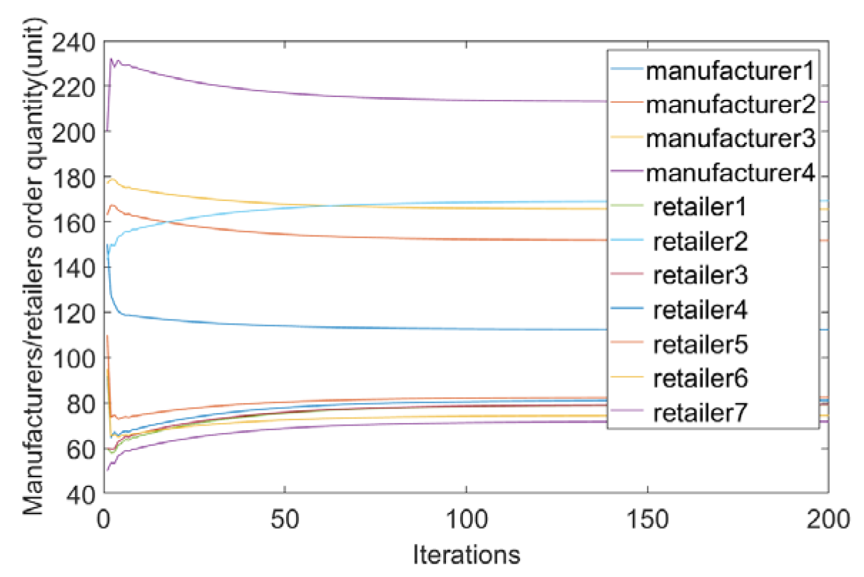
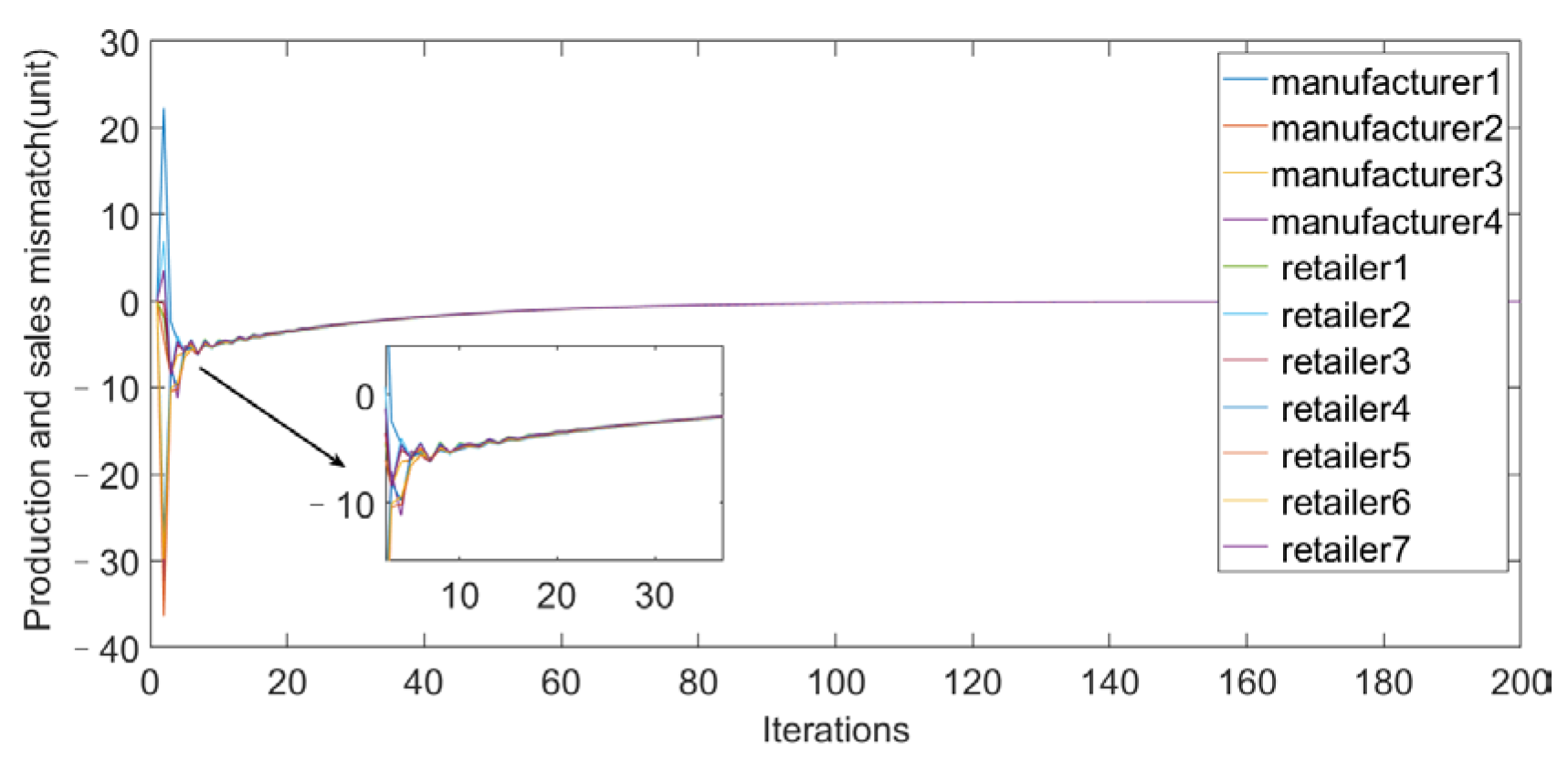
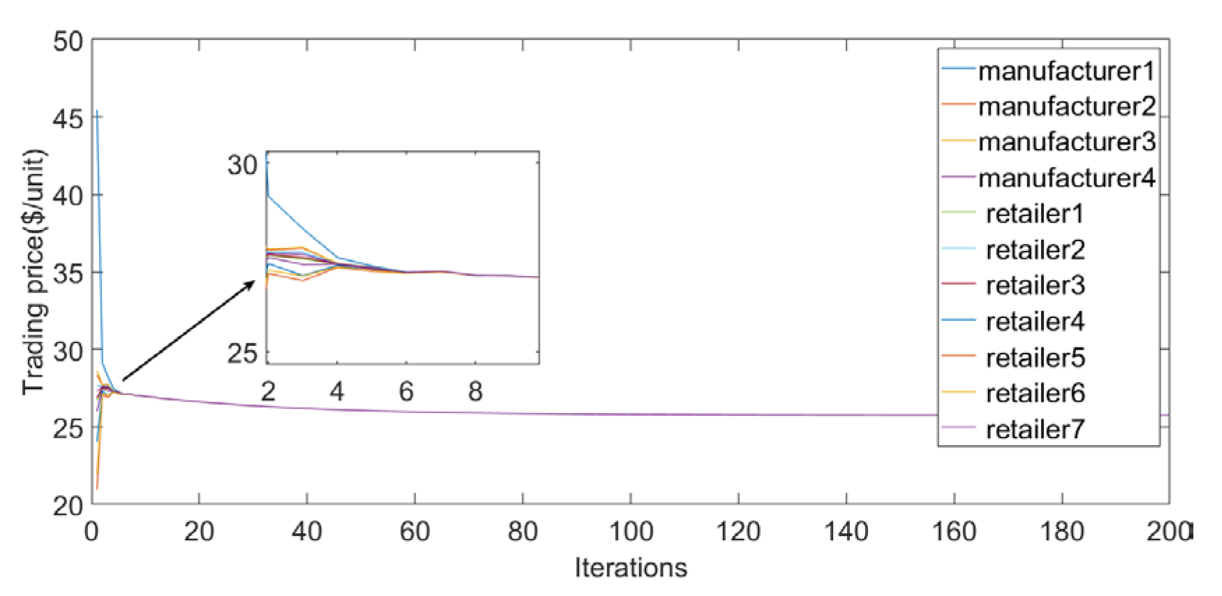
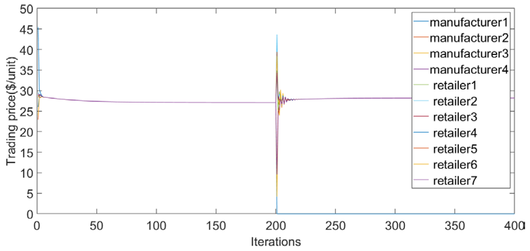
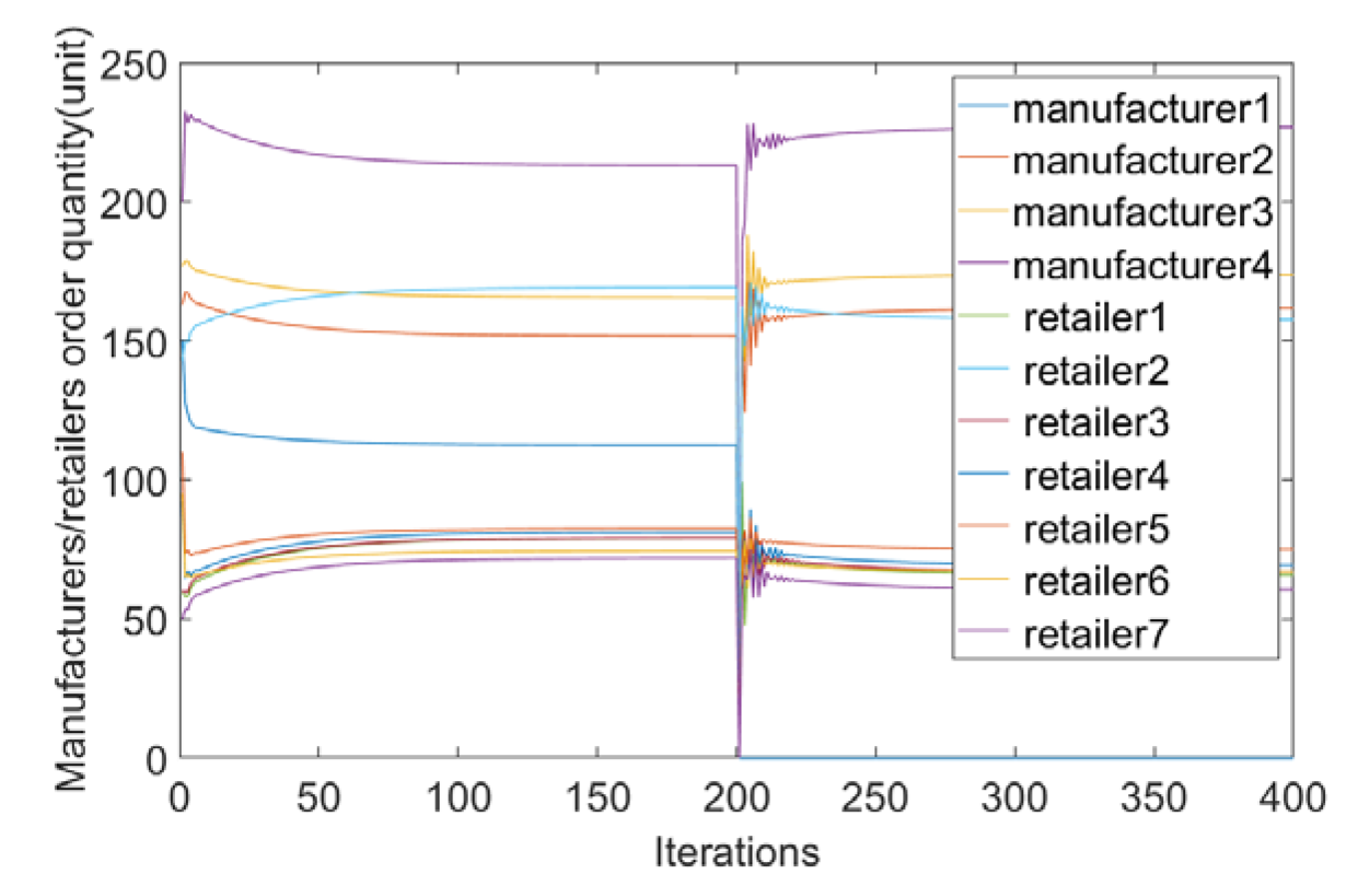
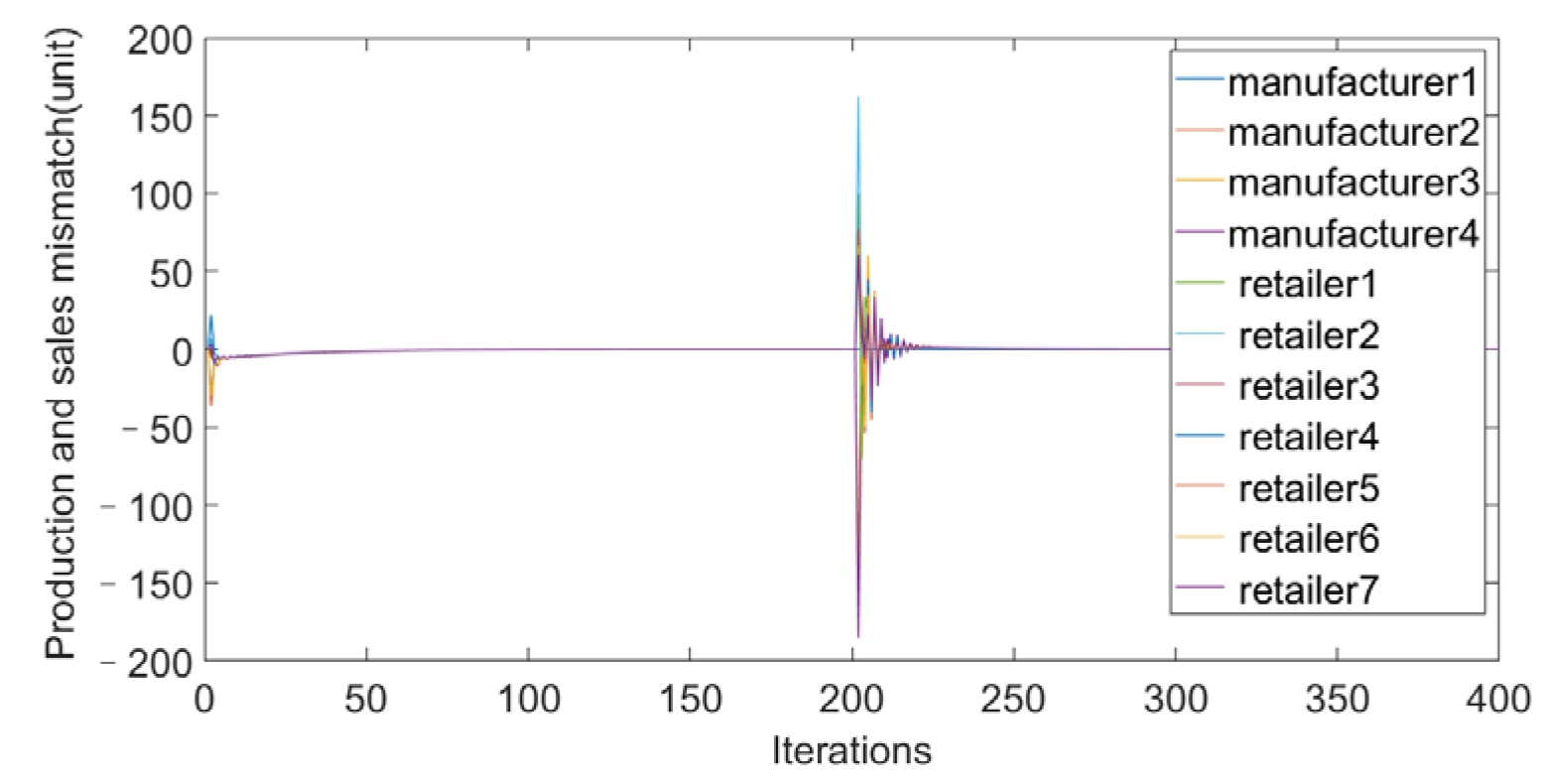
Based on the consensus variables chosen in this paper, the convergence is 27.079 $ / u n i t , as shown in Figure 2, which means that the trading price reaches consensus, and the global optimal level of social welfare is achieved when meeting the supply–demand balance. As seen in Figure 3, the quantities of the retailer and the manufacturer are convergent, and the quantity meets the upper and lower limit constraints and supply–demand balance conditions. Figure 4 depicts that the level of the power mismatch converges to 0; that is, the supply chain is stable and the algorithm is feasible. In addition, the existence of a random delay does not affect the final consensus trading price, nor does it affect the optimality of the transaction quantity.
B. Influence of the sensitivity coefficient
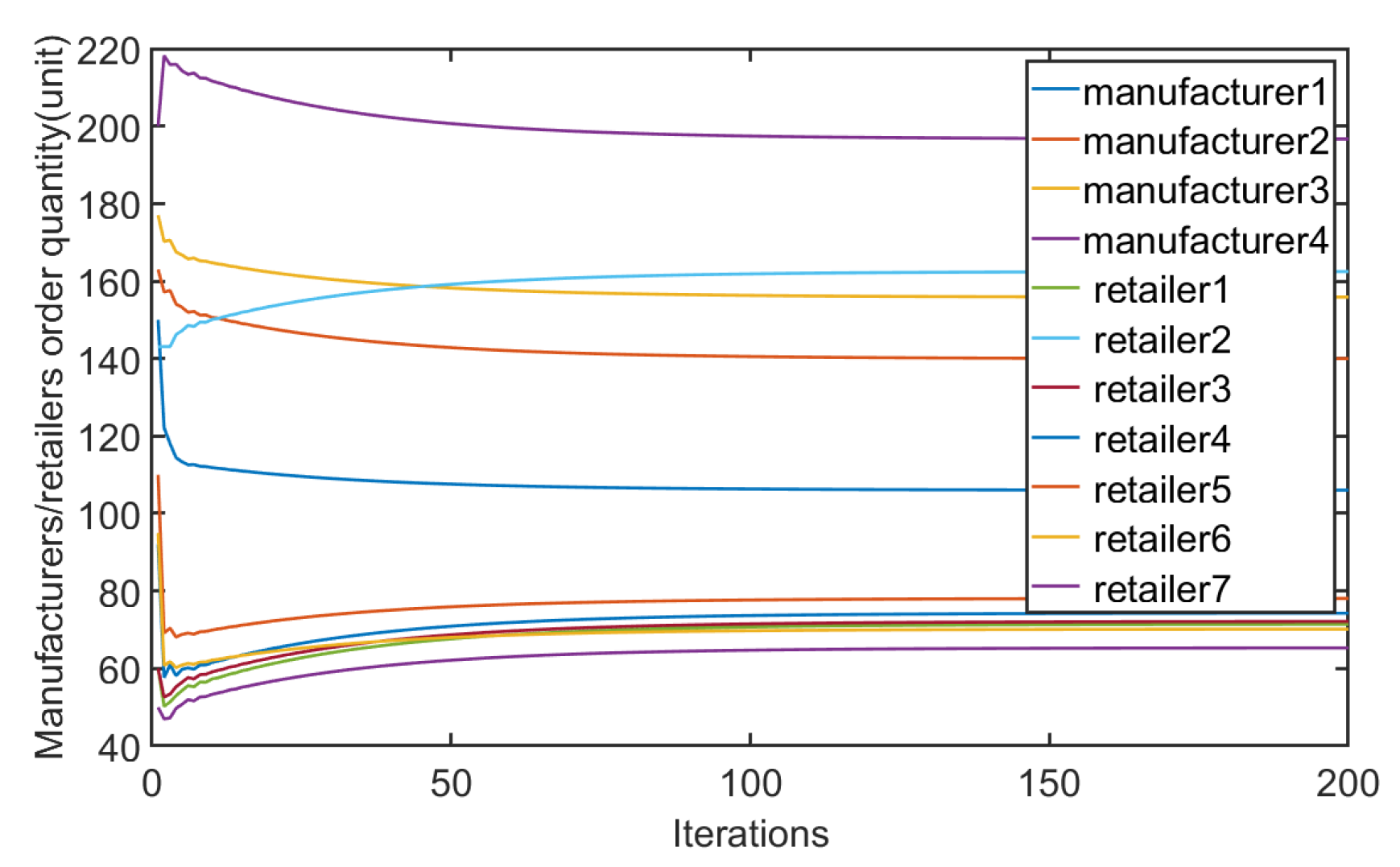
The consumer sensitivity coefficient refers to the sensitivity of consumers to product price changes. According to (6), the change in the sensitivity coefficient affects the price and quantity. Generally, the higher the consumer sensitivity coefficient, the more sensitive consumers are to price changes. The consumer sensitivity coefficient has an impact on sales and prices. As shown in Figure 5 and Figure 6, when the price sensitivity coefficient, γ , increases, the price converges to 25.7387 $/unit. Therefore, retailers expect the demand to increase. Figure 7 verifies that the level of power mismatch converges to 0, that is, the supply chain is stable and the algorithm is feasible. This shows that enterprises need to pay attention to the reactions of consumers when pricing and control the price as far as possible within the acceptable range of consumers. If the price is too high, consumers may choose other alternatives or give up buying the product; on the other hand, despite attracting more consumers, a too-low price will cause losses to the profits of enterprises. Therefore, enterprises need to set product prices reasonably, according to the consumer sensitivity coefficient.
C. Algorithm scalability
Without the loss of generality, it is assumed that Manufacturer 1 suffers a production interruption when the number of iterations is 200 and the remaining manufacturers continue to produce normally. From Figure 8, it can be seen that the convergence degree of the consistency variable is 28.2125. From Figure 9 and Figure 10, it can be concluded that the output of retailers and manufacturers also quickly adjusts and converges, reformulating production and procurement plans. The designed consistency scheme enables the market to enter a stable operation after rapid adjustment and quickly handles the impact of Manufacturer 1, reflecting the scalability of the algorithm.

5. Conclusions

This paper considers a two-echelon supply chain network design problem. Being multi-manufacturer and multi-retailer in nature, the social welfare of suppliers and customers is maximized as much as possible, and the supply chain management problem is described as a consensus control problem in multi-intelligent systems. A price consistency algorithm for obtaining the optimal profit of the supply chain is proposed, and the random delay problem in the design process is considered. The algorithm is theoretically analyzed and numerically verified. The main conclusions are as follows:
(1)
The interests of each node in the supply chain are regarded as a whole and are boiled down to an optimal problem. A multi-agent consensus algorithm suitable for the supply chain is developed considering the random delay of distributed unit communication, and the optimal transaction price and order quantity of the supply chain are determined.
(2)
Changes in sensitivity factors have an impact on both price and quantity. The retailer increases the expected demand according to (6), and the price changes inversely. When the sensitivity coefficient decreases, the expected demand and the consistent price increase, which leads the manufacturer to increase the output under the constraint of supply and demand balance (11), to maximize the overall supply chain benefit. Therefore, setting a reasonable price is the premise for ensuring the profits of retailers and manufacturers.
(3)
When a manufacturer or retailer in the supply chain network fails in a sudden situation, the transaction price will increase and the overall profit will decrease, indicating that supply chain members should cooperate with each other in order to avoid the loss of market profit.
This paper does not take into account some parameters within the model. For example, market demand changes are relatively stable, but there are occasional small fluctuations. Moreover, retailers need to prepare a certain amount of spare inventory to cope with the impact of occasional fluctuations. Furthermore, the reliability of transportation, i.e., the reliability of logistics in the market, is not considered. These limitations will affect the uncertainty of market demand, which is reflected in the system model with uncertainty in the retailer efficiency function model. These problems will be analyzed and discussed in future work.

Author Contributions

Methodology, Y.L.; Writing—original draft, J.W. All authors have read and agreed to the published version of the manuscript.

Funding

This work was supported by Hebei Social Science Fund under Grant HB22GL024.

Data Availability Statement

Not applicable.

Conflicts of Interest

The authors declare no conflict of interest.

Appendix A

To analyze the convergence of the proposed algorithm, the following two lemmas are introduced:
Lemma 1. 
[31] If the matrix A  is written as a blocked lower triangular matrix, that is 
A ˜ = A ˜ 1 0 A ˜ 2 A ˜ 3 ,  
 the set of eigenvalues of  A ˜  is  λ ( A ˜ ) and the eigenvalue sets of  A ˜ 1  and  A ˜ 3  are  λ ( A ˜ 1 )  and  λ ( A ˜ 3 ) respectively; then there is  λ ( A ˜ ) = λ ( A ˜ 1 ) λ ( A ˜ 3 ) .
Lemma 2 
[32] The Perron Frobenius theorem: If a matrix is an irreducible matrix, then it must have a nonnegative real eigenvalue,  X ˜ p f All eigenvalues of this matrix are less than or equal to the nonnegative real eigenvalue,  X ˜ p f If the irreducible matrix is primitive, then X ˜ p f  is a single root eigenvalue. If, and only if, the associated eigenvector of the eigenvalue  X ˜ s  of the irreducible matrix makes  V  all elements of  V ˜ = [ v ¯ 1 v ¯ r ] T , v ¯ n R , n [ 1 , r ]  greater than 0, there is  X ˜ s = X ˜ p f .
τ M = max { τ i j } , ( i , j ) E indicates the maximum delay within all communication paths. When the number of iterations in the iterative process is greater than τ M , the following expansion system is written based on the consistency variable model and the supply–demand mismatch function for each node in Section III:
λ ( k + 1 ) = W 0 λ ( k ) + W 1 λ ( k 1 ) + + W τ M λ ( k τ M ) + η ξ ( k )
λ ( k ) = λ ( k )
λ ( k τ M + 1 ) = λ ( k τ M + 1 )
ξ i ( k + 1 ) = S 0 ( k ) ξ ( k ) + S 1 ( k ) ξ ( k 1 ) + + S τ M ( k ) ξ ( k τ M ) + Q ( k ) Q ( k + 1 ) , i M
ξ i ( k + 1 ) = T 0 ( k ) ξ ( k ) + T 1 ( k ) ξ ( k 1 ) + + T τ M ( k ) ξ ( k τ M ) + D ( k ) D ( k + 1 ) , i R
ξ i ( k ) = ξ i ( k ) , i M
ξ i ( k ) = ξ i ( k ) , i R
ξ i ( k τ M + 1 ) = ξ i ( k τ M + 1 ) , i M
ξ i ( k τ M + 1 ) = ξ i ( k τ M + 1 ) , i R
W 0 , W 1 , W τ M , S 0 , S 1 , S τ M and T 0 , T 1 , T τ M are coefficients of the expanded system, corresponding to the node consistency variables and the degree of the supply–demand mismatch, respectively, and the sum of W 0 , W 1 , W τ M is 1.
Then, the multi-agent supply chain system can be expressed as follows:
λ M ( k + 1 ) λ R ( k + 1 ) ξ M ( k + 1 ) ξ R ( k + 1 ) = A M 1 0 A M 2 0 0 A R 1 0 A R 2 B M 1 0 B M 2 0 0 B R 1 0 B R 2 λ M ( k ) λ R ( k ) ξ M ( k ) ξ R ( k )
A * 1 = W * 0 W * 1 W * τ M I 0 0 0 0 0 0 0 I I 0
A * 2 = η I * 0 0 0 0 0 0 0 0 0 0 0
λ M and λ R are the consensus variables of the retailer node and the manufacturer node at time k , respectively. Matrix A * 1 is the pattern of the matrix A M 1 and A R 1 in system (A10). W * 0 , W * 1 , , W * τ M are coefficient matrices of A M 1 and A R 1 , corresponding to the expansion system (A1)–(A3) with the same number of dimensions as the retailer node and the manufacturer node, respectively. Matrix A * 2 is the format of A M 1 and A R 1 matrices in system (A10). I * is the unit matrix with the same dimensions as A M 1 and A R 1 :
β i = 1 2 α i , i M 1 2 α i , i R
α i = β i 2 α i , i M β i 2 α i , i R
B * 1 = β ( I W 0 ) β ( W 1 ) β ( W τ M ) 0 0 0 0 0 0 0 0 0 0
B * 1 = S 0 η β S 1 S τ M I 0 0 0 0 0 0 I 0 o r T 0 η β T 1 T τ M I 0 0 0 0 0 0 I 0
where β is a matrix, with β as diagonal elements, and the remaining elements are 0.
The coefficient matrix of system (A10) is denoted as A , and the component block matrix is divided. Consider matrix A as matrix A 0 disturbed by matrix H . The eigenvalues of A 0 and the effect of matrix H on the eigenvalues of matrix A 0 should be analyzed separately. Thus, the following decomposition is carried out:
A = A 0 + η H
A 1 A 2 B 1 B 2 = A 1 0 B 1 B 2 * + η 0 I ˜ 0 β ˜
I ˜ = I 0 0 0 0 0 0 0 0 0 0 0 0 0 0 0 0 0 0 0 I 0 0 0 0 0 0 0 0 0 0 0 0 0
β ˜ = β 0 0 0 0 0 0 0 0 0 0 0 0 0 0 0 0 0 0 0 β 0 0 0 0 0 0 0 0 0 0 0 0 0
In this case, B * 2 * in (A18) contains two diagonal chunk matrix elements as B M 2 * and B R 2 * , the format of the two matrices is represented by B * 2 * , and the expression is as follows:
B * 2 * = S * 0 S * 1 S * τ M I 0 0 0 0 0 0 I 0 or T * 0 T * 1 T * τ M I 0 0 0 0 0 0 I 0
S * 0 , S * 1 , , S * τ M and T * 0 , T * 1 , , T * τ M are the coefficient matrices of B M 2 * and B R 2 * , corresponding to the expansion system (A4)–(A9) with the same number of dimensions as the retailer node and the manufacturer node, respectively.
Since A 0 is a blocked lower triangular matrix, its eigenvalues are the concatenated set of A 1 and B 2 * eigenvalues according to Lemma 1. A 1 is a row random matrix and all elements are positive, and the graph topology of the system is strongly connected; therefore, A 1 has a single root eigenvalue of 1, and the other eigenvalues are less than 1.
Let ψ satisfy 1 T ψ = 1 and ϕ = [ 1 N × 1 , , 1 N × 1 ] , and they denote the left and right eigenvectors corresponding to matrix A 1 , respectively; then, 1 N × 1 denotes the column vector of dimension N .
From the form of matrix B 2 * , we can see that B 2 * is an irreducible matrix, and from Lemma 2, we can prove that 1 is the unique maximum eigenvalue of B 2 * .
The following relationships are thus provided:
B 2 * z = z
z = [ z M 1 z M τ M z R 1 z R τ M ]
Solving (A23) yields all Z-normalized values for the right eigenvector of matrix B 2 * . Similarly,
y T = [ y M 1 T y M τ M T z R 1 T z R τ M T ]
y T B 2 * = y T
The left eigenvector of matrix B 2 * can be obtained by calculating all y T values according to (A25).
The above analysis shows that A 0 has two eigenvalues equal to 1. Let X ^ 1 X ^ 2 = 1 . The eigenvector α ˜ 1 , α ˜ 2 β ˜ 1 T β ˜ 2 T should be constructed as the independent left and right eigenvectors of the matrix A 0 . They are expressed as follows:
U ˜ = α ˜ 1 α ˜ 2 = 0 φ θ z ς z
V ˜ T = β ˜ T β ˜ T = φ T β ˜ y T ψ T 0 T
They satisfy V ˜ T U ˜ = I , where
ς = ω = 1 N r = 1 N β ˜ ω r y T Z
θ = 1 y T Z
According to the matrix eigenvalue perturbation theory,
V ˜ T H U ˜ = 0 0 θ ψ T z ς ψ T z
From the Formula (A30), it can be seen that the two eigenvalues of the matrix are 0 and ς ψ T z , so d x ^ 1 d ε = 0 and d x ^ 2 d ε = ς ψ T z < 0 . That is, the first eigenvalue 1 of matrix A 0 is not affected by the disturbance matrix H . When the step size is adequate, the second eigenvalue 1 will gradually decrease under the influence of H . Therefore, it can be concluded that matrix A has a unique eigenvalue 1, and the modulus of other eigenvalues are less than 1. Therefore,
λ M ( k ) λ R ( k ) ξ M ( k ) ξ R ( k ) = A k λ M ( 0 ) λ R ( 0 ) ξ M ( 0 ) ξ R ( 0 ) A * λ M ( 0 ) λ R ( 0 ) 0 0
where λ is a fixed value, and λ M ( 0 ) , λ R ( 0 ) , are the initial values of the consistent variable. When k , i V , lim k λ i ( k ) = λ * and lim k ε i ( k ) = 0 .
The differential forms of the objective function in problem (10), with respect to Q i and D i , are Formulas (14) and (15), respectively. They are the increasing functions of Q i and D i since they are linearly related to λ , Q i , and D i , which converge when λ converges. Optimization problem (10) reaches its minimum value, and the optimal solution satisfies lim k Q i ( k ) = Q i * , i M and lim k D i ( k ) = D i * , i R . Therefore, the algorithm converges, and Theorem 1 is proved.
The convergence of the system is affected by the eigenvalue ς ψ T z of (A30), which is in turn related to the maximum value τ M of the communication delay of the system. The larger τ M increases, increasing ς ψ T z , while the slower eigenvalue X ^ 2 = 1 becomes smaller. The communication system time delay has randomness, and the larger the time delay is, the slower the convergence speed is, and the more difficult it is to guarantee the convergence. Therefore, a sufficiently small η is needed to guarantee the convergence of the system. Considering the extreme case, when all communication delays have their maximum values within the allowed range, the second largest eigenvalue of the system becomes the slowest, and the convergence time reaches the maximum. τ i j = τ i j , max , i V ,   j V , τ M = max { τ i j , max } , i V , j V . At this time, the system is in the most unstable state, and a sufficiently small v exists such that the system converges when 0 < η < v .

References

  1. Savaskan, R.C.; Bhattacharya, S.; Wassenhove, L.N.V. Closed-loop supply chain models with product remanufacturing. Manag. Sci. 2004, 50, 239–252. [Google Scholar] [CrossRef] [Green Version]
  2. Ferguson, M.E.; Toktay, L.B. The effect of competition on recovery strategies. Prod. Oper. Manag. 2010, 15, 351–368. [Google Scholar] [CrossRef] [Green Version]
  3. Shi, T.Q.; Chhajed, D.; Wan, Z.X.; Liu, Y. Distribution channel choice and divisional conflict in remanufacturing operations. Prod. Oper. Manag. 2020, 29, 1702–1719. [Google Scholar] [CrossRef]
  4. Ullah, M.; Asghar, I.; Zahid, M.; Omair, M.; AlArjani, A.; Sarkar, B. Ramification of remanufacturing in a sustainable three-echelon closed-loop supply chain management for returnable products. J. Clean. Prod. 2021, 290, 125609. [Google Scholar] [CrossRef]
  5. Hanh, N.T.M.; Chen, J.M.; Van Hop, N. Pricing strategy and order quantity allocation with price-sensitive demand in three-echelon supply chain. Expert Syst. Appl. 2022, 206, 117873. [Google Scholar] [CrossRef]
  6. Sasan, K.; Mehdi, S.; Bahman, N. A four-echelon supply chain network design with shortage: Mathematical modeling and solution methods. J. Manuf. Syst. 2015, 35, 164–175. [Google Scholar]
  7. Giria, B.C.; Sarker, B.R. Improving performance by coordinating a supply chain with third party logistics outsourcing under production disruption. Comput. Ind. Eng. 2017, 103, 168–177. [Google Scholar] [CrossRef]
  8. Yulin, S.; Simon, C.G.; Xueping, L. An order-splitting model for supplier selection and order allocation in a multi-echelon supply chain. Comput. Oper. Res. 2022, 137, 105515. [Google Scholar]
  9. Feng, W.; Yunquan, D. A Power-Balanced Pareto-Equilibrium Profit Allocation in Supply Chain. IEEE Access 2019, 7, 24889–24897. [Google Scholar]
  10. Xu, G.; Yue, D. Pricing Decisions in a Supply Chain Consisting of One Manufacturer and Two Retailers Under a Carbon Tax Policy. IEEE Access 2021, 9, 3054776. [Google Scholar] [CrossRef]
  11. Chen, T.H. Effects of the Pricing and Cooperative Advertising Policies in a Two-echelon Dual-channel Supply Chain. Comput. Ind. Eng. 2015, 87, 250–259. [Google Scholar] [CrossRef]
  12. Xiao, T.S.J. Pricing and Supply Priority in a Dual-channel Supply Chain. Eur. J. Oper. Res. 2016, 254, 813–823. [Google Scholar] [CrossRef]
  13. Zhao, J.; Hou, X.; Guo, Y.; Wei, J. Pricing Policies for Complementary Products in a Dual-channel Supply Chain. Appl. Math. Model. 2017, 49, 437–451. [Google Scholar] [CrossRef]
  14. Iyer, G.; Villasboas, J.M. A Bargaining Theory of Distribution Channels. J. Mark. Res. 2003, 40, 80–100. [Google Scholar] [CrossRef] [Green Version]
  15. Dukes, A.J.; Galor, E.; Srinivasan, K. Channel Bargaining with Retailer Asymmetry. J. Mark. Res. 2006, 43, 84–97. [Google Scholar] [CrossRef]
  16. Zhang, P.; Xu, X.; Shi, V.; Zhu, J. Simultaneous inventory competition and transshipment between retailers. Int. J. Prod. Econ. 2020, 230, 107781. [Google Scholar] [CrossRef]
  17. Sun, Z.; Xu, Q.; Liu, J. International Journal of Production Economics. Prod. Oper. Manag. 2021, 233, 108011. [Google Scholar]
  18. Zhong, F.; Zhou, Z.; Leng, M. Negotiation-sequence, pricing, and ordering decisions in a three-echelon supply chain: A coopetitive-game analysis. Eur. J. Oper. Res. 2021, 294, 1096–1107. [Google Scholar] [CrossRef]
  19. Ran, W.X.; Xu, T. Low-Carbon Supply Chain Coordination Based on Carbon Tax and Government Subsidy Policy. Sustainability 2023, 15, 1135. [Google Scholar] [CrossRef]
  20. Hossein, M.; Hamed, S.; Keith, W. A robust optimization model for green supplier selection and order allocation in a closed-loop supply chain considering cap-and-trade mechanism. Expert Syst. Appl. 2023, 228, 120423. [Google Scholar]
  21. Yang, H.X.; Chen, X.R.; Li, L. Supply chain decision-making of green products considering a retailer’s fairness concerns under a pre-sale model. J. Clean. Prod. 2023, 414, 137457. [Google Scholar] [CrossRef]
  22. Liu, Z.; Wan, M.D.; Zheng, X.X.; Koh, S.L. Fairness concerns and extended producer responsibility transmission in a circular supply chain. Ind. Market. Manag. 2022, 102, 216–228. [Google Scholar] [CrossRef]
  23. Fox, M.S.; Chionglo, J.F.; Barbuceanu, M. The Integrated Supply Chain Management System; Department of Industrial Engineering, University of Toronto: Toronto, ON, Canada, 1993. [Google Scholar]
  24. Frayret, J.M.; Damours, S.; Rousseau, A.; Harvey, S.; Gaudreault, J. Agent-based supply-chain planning in the forest products industry. Int. J. Flex. Manuf. Syst. 2007, 19, 358–391. [Google Scholar] [CrossRef]
  25. Shen, W.; Norrie, D.H. Agent-based systems for intelligent manufacturing: A state-of-the-art survey. Knowl. Inf. Syst. 1999, 1, 129–156. [Google Scholar] [CrossRef]
  26. Fox, M.S.; Barbuceanu, M.; Teigen, R. Agent-oriented supply-chain management. Int. J. Flex. Manuf. Syst. 2000, 12, 165–188. [Google Scholar] [CrossRef]
  27. Shen, W.; Kremer, R.; Ulieru, M.; Norrie, D. A collaborative agent-based infrastructure for Internet-enabled collaborative enterprises. Int. J. Prod. Res. 2003, 41, 1621–1638. [Google Scholar] [CrossRef]
  28. Ramezani, M.; Bashiri, M.; Reza, T.M. A robust design for a closedloop supply chain network under an uncertain environment. Int. J. Adv. Manuf. Technol. 2013, 66, 825–843. [Google Scholar] [CrossRef]
  29. Olfati-Saber, R.; Fax, J.A.; Murray, R.M. Consensus and cooperation in networked multiagent systems. Proc. IEEE 2007, 95, 215–233. [Google Scholar] [CrossRef]
  30. Zhou, Y.J.; Hu, F.Y.; Zhou, Z.L. Pricing decisions and social welfare in a supply chain with multiple competing retailers and carbon tax policy. J. Clean. Prod. 2018, 190, 752e777. [Google Scholar] [CrossRef]
  31. Colub, G.H.; Van Loan, C.F. Matrix Computations; Posts and Telecom Press: Beijing, China, 2009; pp. 359–363. [Google Scholar]
  32. Meyer, C.D. Matrix Analysis and Applied Linear Algebra; Society for Industrial and Applied Mathematics: Philadelphia, PA, USA, 2000. [Google Scholar]
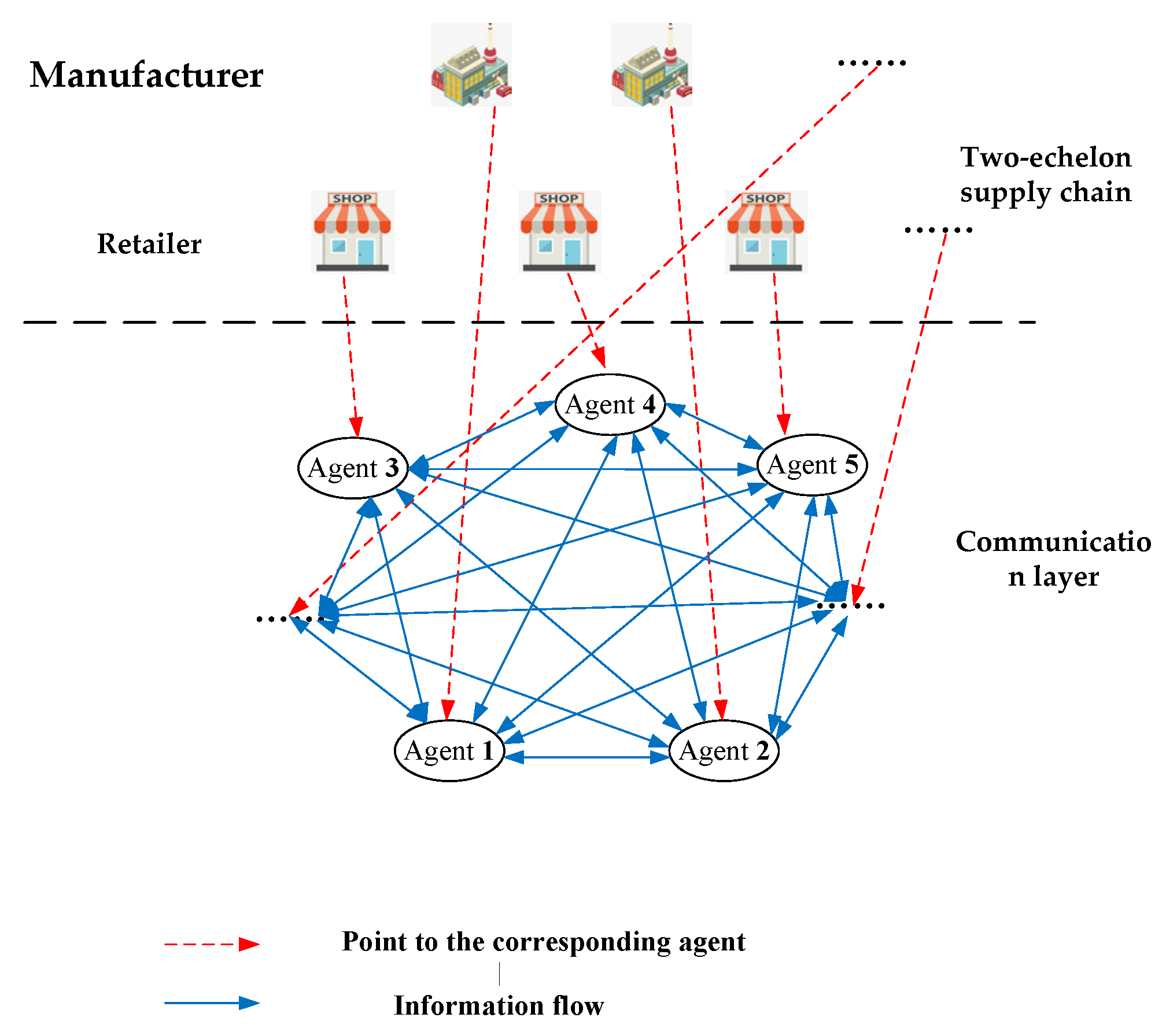
Figure 1. Structure of the two-echelon supply chain multi-agent network.
Sustainability 15 11307 g001
Figure 2. Trading price.
Sustainability 15 11307 g002
Figure 3. Manufacturer/retailer order quantity.
Sustainability 15 11307 g003
Figure 4. Production and sales mismatch.
Sustainability 15 11307 g004
Figure 5. Trading price.
Sustainability 15 11307 g005
Figure 6. Manufacturer/retailer order quantity.
Sustainability 15 11307 g006
Figure 7. Production and sales mismatch.
Sustainability 15 11307 g007
Figure 8. Trading price.
Sustainability 15 11307 g008
Figure 9. Manufacturer/retailer order quantity.
Sustainability 15 11307 g009
Figure 10. Production and sales mismatch.
Sustainability 15 11307 g010
Table 1. Parameters of manufacturer and retailer nodes.
Retailer Parameters
Node α i $ / u n i t 2 β i $ / u n i t D i min ( u n i t ) D i max ( u n i t )
10.04333.80120
20.04943.660190
30.04734.520100
40.04834.870120
50.07539.450120
60.07538.40125
70.05134.4090
Manufacturer Parameters
Node a $ / u n i t 2 b $ / u n i t Q i min ( u n i t ) Q i max ( u n i t )
10.1053.470150
20.0579.780200
30.0694.230200
40.0419.610250
Disclaimer/Publisher’s Note: The statements, opinions and data contained in all publications are solely those of the individual author(s) and contributor(s) and not of MDPI and/or the editor(s). MDPI and/or the editor(s) disclaim responsibility for any injury to people or property resulting from any ideas, methods, instructions or products referred to in the content.