A Fully Decentralized Optimal Dispatch Scheme for an AC–DC Hybrid Distribution Network Formed by Flexible Interconnected Distribution Station Areas

Abstract

Due to unbalanced load growth among different regions and the increasing integration of distributed generators (DGs), distribution station areas (DSAs) currently face issues such as voltage violations, curtailment of renewable energy generation, and imbalanced load rates among DSAs. Interconnecting DSAs to form an AC–DC hybrid distribution network (DN) can not only address the aforementioned problems but also provides more efficient interfaces for DC devices. In order to coordinate the controllable devices within the flexible interconnected DSAs and achieve an optimal operational state, centralized optimal dispatch strategies are mainly used, which requires the deployment of an additional central controller and entails heavy communication and computation burdens. To overcome the drawbacks of centralized dispatch, a fully decentralized optimal dispatch scheme based on the alternating direction method of multipliers (ADMM) is proposed. Based on the network partitioning results, the introduction of auxiliary variables that replicate the coupling variables between areas further eliminates the need for a coordinating center in the standard ADMM, achieving a fully decentralized optimal dispatch. Additionally, two network partitioning methods are proposed for implementing decentralized dispatch. Both partitioning methods can achieve the goals of load rate balance and voltage profile improvement when implementing decentralized dispatch. Their key distinction lies in their effectiveness in improving the voltage profiles on the DC side. The partitioning method that treats the entire DC side as a separate area, resulting in higher investment, achieves better results in improving the DC voltage profiles than the other one. The choice of partitioning method can be based on practical engineering requirements.

1. Introduction

1.1. Background

Distribution substation areas (DSAs) are the endpoint of a distribution network (DN) that directly supply power to the users. They typically refer to the areas powered by a distribution transformer (35 kV/380 V or 10 kV/380 V) [1]. To reduce carbon emissions, an increasing number of distributed generators (DGs), such as photovoltaic (PV) and wind turbines (WTs), are being integrated into the DN [2]. However, this integration also brings forth several challenges. On the one hand, the output power of DGs exhibits strong randomness [3], which can lead to voltage fluctuations [4]. On the other hand, when the output power of DGs exceeds the local load’s consumption capacity, reverse power flow from the DGs to the upstream grid can occur. This can lead to voltage rise in the DSA, and in severe cases, it can cause the voltage to exceed the upper limit. If left unaddressed, this situation can result in widespread disconnection of DGs and damage to electrical equipment, posing a threat to the safe operation of the DSA [5]. To prevent such incidents, measures such as curtailment of wind or solar power are often taken, leading to resource wastage [6]. Additionally, the composition of loads in different DSAs may be different, resulting in load rate imbalance among neighboring DSAs. In some DSAs, due to agricultural or tourism development, the local load exhibits strong seasonal fluctuations. During peak periods of agricultural electricity demand or tourist seasons, the transformers in these DSAs are often operating at heavy loads or even overloads, while during other periods only routine residential loads are present [7]. Meanwhile, the load characteristics in other DSAs may be the opposite. Significant differences in load rates among adjacent DSAs can result in inefficient operation [8]. When there is a significant imbalance in the load rates among adjacent DSAs, some transformers in certain DSAs operate under heavy or even overloaded conditions, while transformers in adjacent DSAs operate under light or moderate loads. Transformers operating under heavy or overloaded conditions not only have limited capacity margins but also face risks such as overheating, increased losses, and shortened lifespan. Meanwhile, transformers operating under light loads have a significant amount of unused capacity. Therefore, when there is a significant imbalance in the load rates among adjacent DSAs, the safety and economic efficiency of the DSAs’ operation need improvement.

However, both the issues caused by mismatch between DG output power and load demand, as well as the problem of load rate imbalance among adjacent DSAs, can be addressed by implementing flexible DC interconnection among neighboring DSAs [9]. Due to the characteristics of fully controlled voltage source converters (VSCs), flexible interconnection devices can facilitate fast and precise power transfer among DSAs [10]. When DG output power cannot be fully consumed locally, it can be transferred to adjacent DSAs for consumption, reducing the occurrence of curtailment measures. Similarly, during transformer overload, a portion of the load can be transferred to DSAs operating at lighter loads, thus relieving the supply pressure on overloaded transformers and improving the capacity utilization of lightly loaded transformers. Furthermore, interconnecting DSAs through flexible DC technology can enable the formation of an AC–DC hybrid DN, providing more efficient DC interfaces for DGs and DC loads [11].

1.2. State of the Art

Currently, flexible DC interconnection technology has gradually been applied in the field of engineering to achieve optimal power flow (OPF) in DNs [12,13]. One important application of this technology is soft open point (SOP) [14], and there have been a lot of studies on achieving DPF in DN based on SOP. The authors in [15] established the OPF model for an islanded DN with SOP, coordinating the power output of DGs and the reactive power compensation of SOP to achieve maximum load capacity. The authors in [16] proposed a control strategy for SOP considering the uncertainty of renewable energy power output, optimizing the power flow in a DN with a high proportion of renewable energy source (RES). The authors in [17] proposed using SOP to address three-phase unbalanced operation issues. The authors in [18] combined energy storage systems (ESS) with SOP to enable the DN to operate closer to its limits and maximize profits. The authors in [19] suggested the use of multi-terminal SOP to alleviate load imbalance on feeders.

In recent years, there has been extensive research on AC–DC hybrid DNs to accommodate the increasing integration of emerging power sources and loads, such as DGs and electric vehicles (EVs). The authors in [20] indicate that AC–DC hybrid distribution technology is crucial for the development of regional energy internet. The authors in [21] proposed a novel two-stage hybrid method for managing the power consumption of residential buildings with a hybrid AC–DC electricity supply. The authors in [22] point out that an automated demand response will play a significant role in future distribution networks. By providing the right incentives, generators and consumers can be encouraged to activate their flexibilities, thereby increasing the hosting capacity of the distribution system.

The above studies provide valuable insights into the optimal dispatch of an AC–DC hybrid DN formed by flexible interconnected DSAs, but they cannot be directly applied to optimize the operation of flexible interconnected DSAs, as their objectives do not include the term of load rate balancing among DSAs.

In order to utilize flexible DC interconnection technology to achieve power transfer among DSAs and address issues such as incomplete local consumption of DG output power and load rate imbalance among DSAs, The authors in [9] proposed a dispatch scheme for an AC–DC hybrid DN based on flexible interconnection, with the goal of load rate balancing among DSAs. The authors in [23] further considered the impact of flexible interconnection devices’ control mode on the DC voltage deviation in an AC–DC hybrid DN. It can further reduce the voltage deviation on the DC side and effectively improve the voltage profile while balancing the load rate among DSAs. However, it is important to note that the studies mentioned above used a centralized dispatch scheme that relies on global information from the whole DN for operation optimization, which imposes significant communication and computational burdens. Additionally, implementing a centralized optimal dispatch scheme requires a central controller capable of collecting and processing global information. Considering the low voltage level (380 V) of DSAs, the control of specific devices within the DSAs is typically not within the jurisdiction of the distribution network’s dispatch center. Therefore, implementing a centralized scheme in flexible interconnected DSAs would require deploying an additional central controller, which is not cost-effective.

Given the drawbacks of centralized dispatch, research on decentralized dispatch has gained attention in the field. The authors in [24] propose the use of a deep reinforcement learning model for indirect multi-energy trading. However, on the one hand, deep reinforcement learning is a model-free method typically employed in scenarios where it is challenging to establish accurate models. On the other hand, deep reinforcement learning models require a large amount of data for training. This not only incurs significant costs in data set construction but also entails substantial computational overhead during the training process. Therefore, for the optimal dispatch problem in the flexible interconnected DSAs, adopting deep reinforcement learning methods would not be appropriate. The same applies to the federated reinforcement learning approach employed in [25]. In [26], a decentralized model predictive control method is used to control hybrid distribution transformers for voltage regulation in the DN. However, this decentralized control technology is not applicable to flexible interconnected DSAs. Because there is no communication among the local controllers of different areas, it would not be possible to know the load rate of other DSAs, thus hindering the achievement of load rate balancing among the DSAs. The authors in [27] proposed a distributed OPF model for hybrid AC–DC microgrids based on power electronic transformers. However, the power electronic transformers act as coordinating centers, and the scheme does not achieve full decentralization.

To provide a clear comparison of the aforementioned studies,

Table 1. Summary of the key aspects of the studies.

Ref. No.	Dispatch Scheme	Objective
[15,16,18]	Centralized	Optimal power flow
[17]	Centralized	Address three-phase imbalance
[9,19,23]	Centralized	Address load rate imbalance
[24]	Decentralized	Indirect multi-energy trading
[25,26]	Decentralized	Voltage regulation
[27]	Decentralized	Optimal power flow

provides a summary of their key aspects.

The purpose of the work is to propose a decentralized dispatch scheme suitable for flexible interconnected DSAs, which can achieve the operation objective while alleviating the communication and computation burden. Additionally, since measurement and control terminals (MCTs) and edge computing devices (ECDs) are typically deployed in DSAs for local measurement and control purposes, they can be utilized for decentralized computation without the need for additional decentralized computing devices in each area. Therefore, compared to centralized control, decentralized control can be more cost-effective. The alternating direction method of multipliers (ADMM), a widely used decentralized algorithm [28], is employed to implement the decentralized dispatch.

The main contributions are twofold:

(1)

A fully decentralized dispatch scheme suitable for flexible interconnected DSAs is proposed, which significantly reduces the communication and computation burden while achieving the same objectives as centralized dispatch.

(2)

Two network partitioning methods are proposed corresponding to the two communication architectures for implementing the decentralized dispatch. One architecture cannot achieve the optimal control mode selection of the converter station, which can further reduce the voltage deviation on the DC side, but it does not require the additional deployment of MCTs and ECDs on the DC side. The other architecture incorporates the control modes of the converter stations into the control model, allowing for optimal voltage profiles on the DC side. However, this architecture requires the installation of an additional MCT and ECD on the DC side, resulting in increased investment. The choice of the appropriate decentralized communication architecture can be made based on the specific requirements in practical engineering applications.

The remainder of this paper is organized as follows. Section 2 describes the original centralized dispatch scheme and presents the centralized communication architecture. Section 3 derives the decentralized dispatch scheme based on ADMM and proposes two decentralized communication architectures for implementing the decentralized dispatch. Section 4 verifies the effectiveness of the decentralized dispatch scheme under the two communication architectures. Section 5 summarizes the whole paper.

2. Original Centralized Dispatch Scheme

2.1. Centralized Dispatch Model

In order to address the issues of load rate imbalance and voltage violations within DSAs through flexible DC interconnection technology, a centralized control scheme is proposed, which aims to obtain the control scheme for dispatchable devices in AC–DC hybrid DNs by solving the following optimization model.

2.1.1. Objective Function

Taking into consideration the issue of load rate imbalance among DSAs and the safe and economic operation of the DN, the objective function encompasses three components: load rate balancing among DSAs, voltage deviations, and the operational cost.

$$\min F={\alpha }_1\frac{f_1}{s_1}+{\alpha }_2\frac{f_2}{s_2}+{\alpha }_3\frac{f_3}{s_3}$$

(1)

Here, f₁ denotes the extent of load rate imbalance among DSAs; f₂ denotes the extent of voltage deviations across the entire DN; f₃ represents the operational cost; s₁, s₂, and s₃ are the baseline values for f₁, f₂, and f₃, respectively, representing the value without optimization; and α₁, α₂, and α₃ are the weight coefficients for the three components, respectively.

The expressions of f₁, f₂, and f₃ are as follows:

$$f_1=\sum _{t\in T}\sum _{d\in D}\left|\frac{P_{d,t}}{S_d}-\frac{1}{n_{\mathrm{d}}}\sum _{d\in D}\frac{P_{d,t}}{S_d}\right|$$

(2)

where t denotes the time point, T denotes the set of dispatch periods, d is the index of DSAs, S_d denotes the capacity of the transformer in DSA-d, D denotes the set of DSAs, P_d,t denotes the value of active power flowing through the transformer in DSA-d at time t, and n_d denotes the amount of DSAs.

$$f_2={\displaystyle \sum _{t\in T}{\displaystyle \sum _{j\in \mathcal{N}}\left|v_{j,t}-{\left(U_{\mathrm{N}}\right)}^2\right|}}$$

(3)

Here, $\mathcal{N}$ denotes the set of nodes in the DN, j is the index of nodes, v_j,t denotes the squared value of the voltage magnitude at node j at time t, and U_N denotes the rated voltage.

$$f_3=c_{\mathrm{loss}}{\displaystyle \sum _{t\in T}{\displaystyle \sum _{ij\in \mathsf{\Omega }}{l}_{ij,t}{r}_{ij}\Delta t}}+c_{\cos \mathrm{t}}{\displaystyle \sum _{t\in T}{\displaystyle \sum _{d\in D}{P}_{d,t}\Delta t}}+c_{\mathrm{cur}}{\displaystyle \sum _{t\in T}{\displaystyle \sum _{j\in {\mathcal{N}}^{\mathrm{PV}}}\left(P_{j,t}^{\mathrm{PV}, \max }-P_{j,t}^{\mathrm{PV}}\right)\Delta t}}$$

(4)

Here, c_loss denotes the unit cost of power losses, ij denotes the branch from between node i and node j, Ω denotes the set of branches, l_ij,t denotes the squared value of the current magnitude, r_ij denotes the resistance of branch ij, Δt denotes the time interval, c_cost denotes the unit cost of purchasing electricity from the superior power grid, c_cur denotes the unit penalty cost of PV output curtailment, ${\mathcal{N}}^{\mathrm{PV}}$ denotes the set of nodes connected to PV, $P_{j,t}^{\mathrm{PV}}$ denotes the active power injected by PV, and $P_{j,t}^{\mathrm{PV},\max }$ denotes the maximum active power output of PV.

2.1.2. Constraints

(1)

AC power flow constraints are as follows [29]:

$$\sum _{ij\in {\mathsf{\Omega }}_j^{\mathrm{U}}}\left(P_{ij,t}-r_{ij}{l}_{ij,t}\right)+P_{j,t}=\sum _{jk\in {\mathsf{\Omega }}_j^{\mathrm{D}}}{P}_{jk,t}$$

(5)

$$\sum _{ij\in {\mathsf{\Omega }}_j^{\mathrm{U}}}\left(Q_{ij,t}-x_{ij}{l}_{ij,t}\right)+Q_{j,t}=\sum _{jk\in {\mathsf{\Omega }}_j^{\mathrm{D}}}{Q}_{jk,t}$$

(6)

$$v_{i,t}-v_{j,t}+\left(r_{ij}^2+x_{ij}^2\right)l_{ij,t}-2\left(r_{ij}{P}_{ij,t}+x_{ij}{Q}_{ij,t}\right)=0$$

(7)

$${\Vert \begin{array}{c}2P_{ij,t}\\ 2Q_{ij,t}\\ l_{ij,t}-v_{i,t}\end{array}\Vert }_2\le l_{ij,t}+v_{i,t}$$

(8)

$$P_{j,t}=P_{j,t}^{\mathrm{PV}}+P_{j,t}^{\mathrm{ESS}, \mathrm{dis}}-P_{j,t}^{\mathrm{ESS}, \mathrm{ch}}+P_{j,t}^{\mathrm{VSC}, \mathrm{AC}}-P_{j,t}^{\mathrm{load}}$$

(9)

$$Q_{j,t}=Q_{j,t}^{\mathrm{PV}}+Q_{j,t}^{\mathrm{VSC}, \mathrm{AC}}-Q_{j,t}^{\mathrm{load}}$$

(10)

$${\left({\underset{\_}{U}}^{\mathrm{AC}}\right)}^2\le v_{j,t}\le {\left({\overline{U}}^{\mathrm{AC}}\right)}^2$$

(11)

$$0\le l_{ij,t}\le {\left(I_{\max }^{\mathrm{AC}}\right)}^2$$

(12)

where ${\mathsf{\Omega }}_j^{\mathrm{U}}$ denotes the set of upstream branches of node j, ${\mathsf{\Omega }}_j^{\mathrm{D}}$ denotes the set of downstream branches of node j, $P_{ij,t}$ and $Q_{ij,t}$ denote the active and reactive power flows of branch ij at time t, P_j,t and Q_j,t denote the total injected active and reactive power at node j at time t, x_ij denotes the reactance of branch ij, $Q_{j,t}^{\mathrm{PV}}$ denotes the reactive power injected by PV, $P_{j,t}^{\mathrm{ESS}, \mathrm{ch}}$ and $P_{j,t}^{\mathrm{ESS}, \mathrm{dis}}$ denote the charging and discharging power, $P_{j,t}^{\mathrm{VSC},\mathrm{AC}}$ and $Q_{j,t}^{\mathrm{VSC},\mathrm{AC}}$ denote the injected active and reactive power on the AC side by the VSC, $P_{j,t}^{\mathrm{load}}$ and $Q_{j,t}^{\mathrm{load}}$ denote the active and reactive power consumption of the load, ${\underset{\_}{U}}^{\mathrm{AC}}$ and ${\overline{U}}^{\mathrm{AC}}$ denote the lower and upper limits of the desired voltage range on the AC side, and $I_{\max }^{\mathrm{AC}}$ denotes the upper limit of current on the AC side.

(2)

DC power flow constraints are as follows [30]:

$$\sum _{ij\in {\mathsf{\Omega }}_j^{\mathrm{U}}}\left(P_{ij,t}-r_{ij}{l}_{ij,t}\right)+P_{j,t}=\sum _{jk\in {\mathsf{\Omega }}_j^{\mathrm{D}}}{P}_{jk,t}$$

(13)

$$v_{i,t}-v_{j,t}+r_{ij}^2{l}_{ij,t}-2r_{ij}{P}_{ij,t}=0$$

(14)

$${\Vert \begin{array}{c}2P_{ij,t}\\ l_{ij,t}-v_{i,t}\end{array}\Vert }_2\le l_{ij,t}+v_{i,t}$$

(15)

$$P_{j,t}=P_{j,t}^{\mathrm{PV}}+P_{j,t}^{\mathrm{ESS}, \mathrm{dis}}-P_{j,t}^{\mathrm{ESS}, \mathrm{ch}}+P_{j,t}^{\mathrm{VSC}, \mathrm{DC}}-P_{j,t}^{\mathrm{load}}$$

(16)

$${\left({\underset{\_}{U}}^{\mathrm{DC}}\right)}^2\le v_{j,t}\le {\left({\overline{U}}^{\mathrm{DC}}\right)}^2$$

(17)

$$0\le l_{ij,t}\le {\left(I_{\max }^{\mathrm{DC}}\right)}^2$$

(18)

where $P_{j,t}^{\mathrm{VSC},\mathrm{DC}}$ denotes the active power injection on the AC side by the VSC, ${\underset{\_}{U}}^{\mathrm{DC}}$ and ${\overline{U}}^{\mathrm{DC}}$ denote the upper and lower limits of the desired voltage range on the DC side, and $I_{\max }^{\mathrm{DC}}$ denotes the upper limit of current on the DC side.

(3)

Suppose the converter station is connected to node n on the AC side and node k on the DC side; the constraints of the converter station are as follows [23]:

$${\left(P_{n, t}^{\mathrm{VSC}, \mathrm{AC}}\right)}^2+{\left(Q_{n, t}^{\mathrm{VSC}, \mathrm{AC}}\right)}^2\le {\left(S^{\mathrm{VSC}}\right)}^2$$

(19)

$$P_{n, t}^{\mathrm{VSC}, \mathrm{AC}}=-P_{k, t}^{\mathrm{VSC}, \mathrm{DC}}$$

(20)

$$0\le U_{n, t}\le \frac{\sqrt{3}}{2\sqrt{2}}{U}_{k, t}$$

(21)

$${\delta }_{k,t}{U}_{\mathrm{N}}^{\mathrm{DC}}+\left(1-{\delta }_{k,t}\right){\underset{\_}{U}}^{\mathrm{DC}}\le U_{k,t}^{\mathrm{DC}}\le {\delta }_{k,t}{U}_{\mathrm{N}}^{\mathrm{DC}}+\left(1-{\delta }_{k,t}\right){\overline{U}}^{\mathrm{DC}} ,\forall k\in {\mathcal{N}}^{\mathrm{VSC}, \mathrm{DC}}$$

(22)

$${\displaystyle \sum _{k\in {\mathcal{N}}^{\mathrm{VSC}, \mathrm{DC}}}{\delta }_{k,t}}=1 ,\forall t$$

(23)

where S^VSC denotes the rated capacity of the converter, δ_k,t denotes the control mode of the converter, δ_k,t = 1 denotes the U_dc-Q control mode, δ_k,t = 0 denotes the P-Q control mode, and ${\mathcal{N}}^{\mathrm{VSC},\mathrm{DC}}$ denotes the set of converters.

(4)

The constraints of ESS are as follows [31]:

$$S_{j,t+1}^{\mathrm{ESS}}=S_{j,t}^{\mathrm{ESS}}+\frac{{\eta }_{\mathrm{ch}}{P}_{j,t}^{\mathrm{ESS}, \mathrm{ch}}\mathsf{\Delta }t}{E_j^{\mathrm{ESS}}}-\frac{P_{j,t}^{\mathrm{ESS}, \mathrm{dis}}\mathsf{\Delta }t}{{\eta }_{\mathrm{dis}}{E}_j^{\mathrm{ESS}}}$$

(24)

$${\underset{\_}{S}}_j^{\mathrm{ESS}}\le S_{j,t}^{\mathrm{ESS}}\le {\overline{S}}_j^{\mathrm{ESS}}$$

(25)

$$S_{j,t=1}^{\mathrm{ESS}}=S_{j,t=24}^{\mathrm{ESS}}$$

(26)

$$0\le P_{j,t}^{\mathrm{ESS}, \mathrm{ch}}\le {\lambda }_{j,t}^{\mathrm{ch}}{P}_{j,t}^{\mathrm{ESS}, \mathrm{ch}, \max }$$

(27)

$$0\le P_{j,t}^{\mathrm{ESS}, \mathrm{dis}}\le {\lambda }_{j,t}^{\mathrm{dis}}{P}_{j,t}^{\mathrm{ESS}, \mathrm{dis}, \max }$$

(28)

$${\lambda }_{j,t}^{\mathrm{dis}},{\lambda }_{j,t}^{\mathrm{ch}}\in \left\{0,1\right\}$$

(29)

$${\lambda }_{j,t}^{\mathrm{dis}}+{\lambda }_{j,t}^{\mathrm{ch}}\le 1$$

(30)

where $S_{j,t}^{\mathrm{ESS}}$ denotes the state of charge (SoC) of the ESS, $E_j^{\mathrm{ESS}}$ denotes the rated capacity of the ESS, η_dis and η_ch denote the discharging and charging efficiency, respectively, ${\underset{\_}{S}}_j^{\mathrm{ESS}}$ and ${\overline{S}}_j^{\mathrm{ESS}}$ denote the lower and upper limits of the SoC, respectively, ${\lambda }_{j,t}^{\mathrm{dis}}=1$ denotes the discharging state, ${\lambda }_{j,t}^{\mathrm{ch}}=1$ denotes the charging state, and $P_{j,t}^{\mathrm{ESS},\mathrm{dis},\max }$ and $P_{j,t}^{\mathrm{ESS},\mathrm{ch},\max }$ denote the upper limits of the discharging and charging power, respectively.

(5)

Constraints of PV are as follows [31]:

$$0\le P_{j,t}^{\mathrm{PV}}\le P_{j,t}^{\mathrm{PV}, \max }$$

(31)

$${\left(P_{j,t}^{\mathrm{PV}}\right)}^2+{\left(Q_{j,t}^{\mathrm{PV}}\right)}^2\le {\left(S_j^{\mathrm{PV}}\right)}^2$$

(32)

where $S_j^{\mathrm{PV}}$ denotes the rated capacity of PV.

(6)

Constraints of the transformer are as follows [9]:

$${\left(P_{d,t}\right)}^2+{\left(Q_{d,t}\right)}^2\le {\left(S_d\right)}^2$$

(33)

where P_d,t denotes the value of reactive power flowing through the transformer in DSA-d at time t.

The mixed-integer second-order cone programming (MISOCP) model, composed of Equations (1)–(33), forms the centralized dispatch model adopted by the centralized dispatch scheme.

2.2. Centralized Communication Architecture

Direct implementation of control using the centralized dispatch model requires the adoption of a centralized communication architecture as shown in Figure 1.

The centralized communication architecture, as shown in Figure 1, was adopted. Measurement and control terminals (MCTs) and edge computing devices (ECDs) were originally deployed within the DSAs to collect and process local data and issue control commands to local devices. After establishing the flexible DC interconnection among DSAs, the converter station and devices on the DC side can also be locally connected to MCTs and ECDs for management. However, since the centralized dispatch model requires simultaneous coordination of multiple DSAs, a central controller is necessary to aggregate information from all DSAs, make decisions, and send control command to MCTs for execution. Due to the low voltage level (380 V) of the DSAs, the control schemes for specific dispatchable devices within these DSAs are typically beyond the jurisdiction of the superior dispatch center. Therefore, an additional central controller is needed to coordinate the dispatch of the entire AC–DC hybrid DN. The central controller needs to communicate with all DSAs and collect and process data from them. Consequently, this centralized communication architecture faces significant communication and computational burdens, as well as additional investments.

3. Decentralized Dispatch Scheme

If dispatch is implemented using a decentralized scheme, based on the originally existing MCTs, ECDs within each DSA, and necessary inter-area communication to solve the dispatch model, it would eliminate the need for a central controller. This approach would greatly reduce computational and communication costs, resulting in reduced investment.

3.1. Transforming Centralized Dispatch Model into Decentralized Dispatch Model

Using a decentralized approach to solve the control model requires the use of distributed algorithms. The ADMM is employed, which first necessitates the transformation of the original centralized dispatch model into a decentralized dispatch model.

Supposing the DN is divided into R areas, the centralized dispatch model introduced earlier can be summarized as the optimization model represented by Equations (34)–(37):

$$obj.\min {\displaystyle \sum _{i=1}^R{f}_i\left(x_i,\widetilde{x_i}\right)}$$

(34)

$$s.t.g_i\left(x_i\right)\ge 0 ,\forall i$$

(35)

$$h_i\left(x_i\right)=0 ,\forall i$$

(36)

$${\displaystyle \sum _{i=1}^R{A}_i\widetilde{x_i}+B=0}$$

(37)

where x_i denotes the vector of decision variables included in the independent constraints of the i-th area, $\widetilde{x_i}$ denotes the vector of decision variables included in the coupling constraints, Equations (35) and (36) represent the independent inequality constraints and equality constraints, respectively, Equation (37) represents the coupling constraints between areas, and if the coupling constraints do not involve the state variables of the i-th area, A_i = 0.

The process of transforming the centralized dispatch model into a fully decentralized dispatch model is as follows.

Duplicate each $\widetilde{x_i}$ in Equation (37) R times as local backups in each area, as shown in Equation (38):

$$\widetilde{x_i^1}=\widetilde{x_i^2}=\cdots =\widetilde{x_i^R}=\widetilde{x_i},\left(i=1,2,\cdots ,R\right)$$

(38)

Let $\widetilde{X^i}={\left[\widetilde{x_1^i},\widetilde{x_2^i},\cdots ,\widetilde{x_R^i}\right]}^{\mathrm{T}},\left(i=1,2,\cdots ,R\right)$, where the vector $\widetilde{X^i}$ consists of the local backup of the variables involved in the coupling constraints from all other areas within the i-th area. By introducing auxiliary variable vectors Z^i,j for the neighboring areas, the Equation (38) can be rewritten as follows:

$$\widetilde{X^1}=Z^{1,2}=\widetilde{X^2}=\cdots =Z^{i-1,i}=\widetilde{X^i}=Z^{i,i+1}=\widetilde{X^{i+1}}\cdots =\widetilde{X^{R-1}}=Z^{R-1,R}=\widetilde{X^R}$$

(39)

Letting $A={\left[A_1,\cdots ,A_R\right]}^{\mathrm{T}}$, the centralized dispatch model represented by Equations (34)–(36) can be transformed into the decentralized dispatch model represented by Equations (40)–(45):

$$obj.\min {\displaystyle \sum _{i=1}^R{f}_i\left(x_i,\widetilde{X^i}\right)}$$

(40)

$$s.t.g_i\left(x_i\right)\ge 0 ,\forall i$$

(41)

$$h_i\left(x_i\right)=0 ,\forall i$$

(42)

$$A\widetilde{X^i}+B=0$$

(43)

$$\widetilde{X^i}=Z^{i,i+1} ,\forall i$$

(44)

$$\widetilde{X^i}=Z^{i-1,i} ,\forall i$$

(45)

From Equations (40)–(45), it can be seen that the decentralized dispatch model only involves local variables within each area and auxiliary variables between neighboring areas. The auxiliary variables can be stored locally, and since they are only coupled with neighboring areas, communication is only required between adjacent areas. This aspect will be further analyzed in subsequent sections.

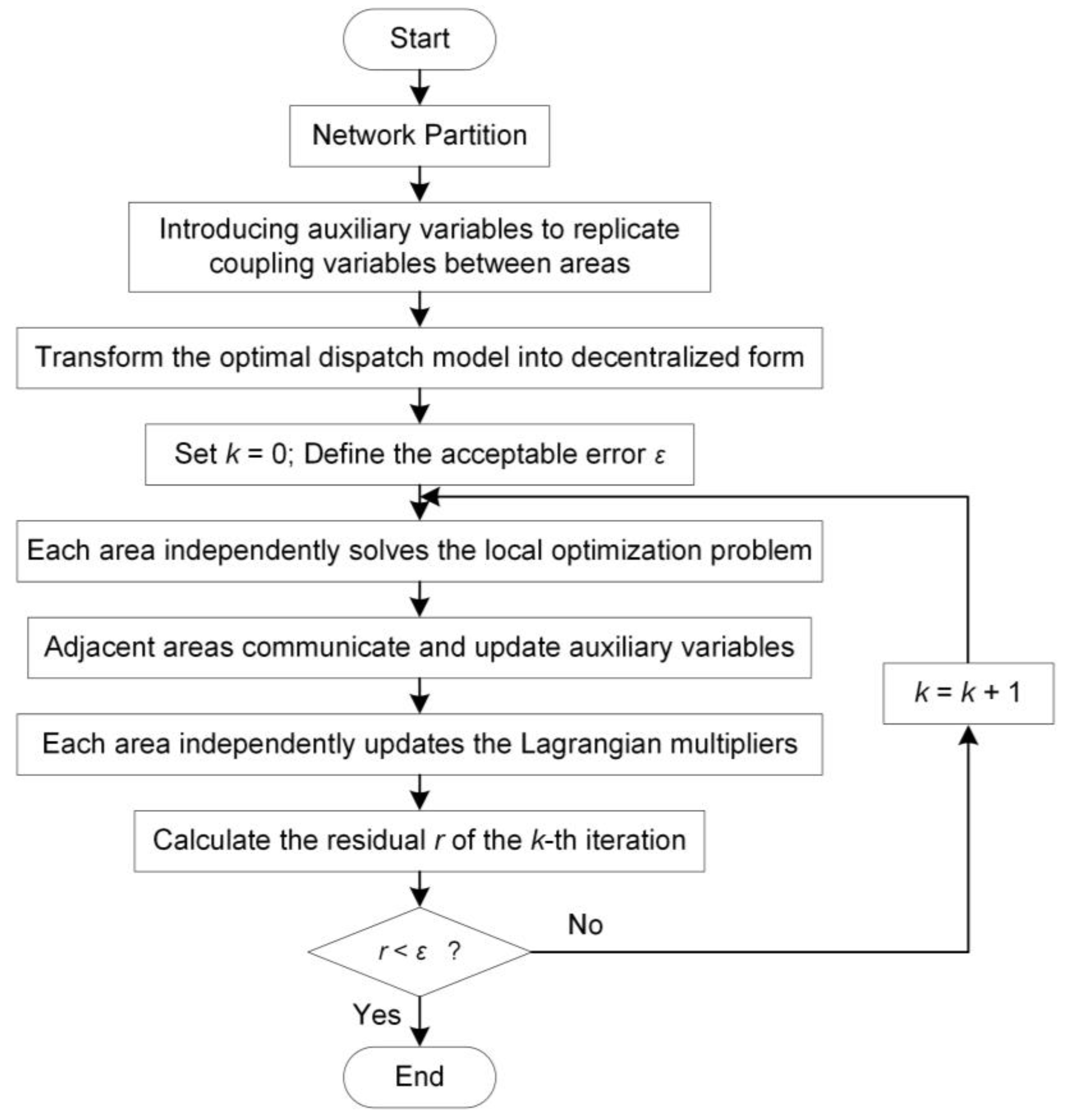
3.2. Solution of the Decentralized Dispatch Model Based on ADMM

After obtaining the decentralized control model, the ADMM is used to solve it. The scaled form of the augmented Lagrangian function for the decentralized dispatch model, with the feasibility sets defined by three constraints (41), (42), and (43) as Fⁱ, is given by:

$$\begin{array}{l}L\left(\left\{x_i,\widetilde{X^i}|\forall i\right\},\left\{Z^{i-1,i},Z^{i,i+1}|\forall i\right\},\left\{w_1^i,w_2^i|\forall i\right\}\right)=\\ {\displaystyle \sum _{i=1}^R{f}_i\left(x_i,\widetilde{X^i}\right)}+\frac{\rho }{2}{\displaystyle \sum _{i=2}^{R-1}{\Vert \begin{array}{l}\widetilde{X^i}-Z^{i-1,i}+w_1^i\\ \widetilde{X^i}-Z^{i,i+1}+w_2^i\end{array}\Vert }_2^2}+\frac{\rho }{2}{\Vert \widetilde{X^1}-Z^{1,2}+w^1\Vert }_2^2+\frac{\rho }{2}{\Vert \widetilde{X^R}-Z^{R-1,R}+w^R\Vert }_2^2, \left(x_i,\widetilde{X^i}\in F^i\right)\end{array}$$

(46)

where ρ denotes the penalty coefficient, and w denotes the vector of the scaling form of Lagrange multipliers.

Based on the Lagrangian function, the specific steps for iteratively solving the above model using the standard two-block ADMM are as follows:

Step 1:

$${\left\{x_i,\widetilde{X^i}|\forall i\right\}}^{\left(k+1\right)}=\underset{x_i,\widetilde{X^i}\in F^i,\forall i}{\arg \min }L\left(\left\{x_i,\widetilde{X^i}|\forall i\right\},{\left\{Z^{i-1,i},Z^{i,i+1}|\forall i\right\}}^{(k)},{\left\{w_1^i,w_2^i|\forall i\right\}}^{(k)}\right)$$

(47)

where k denotes the iteration number.

Note that the local variables within the i-th area are ${\Phi }_i=\left\{x_i,\widetilde{X^i},Z^{i-1,i},Z^{i,i+1},w_1^i,w_2^i\right\}$; therefore, this optimization model shown in Equation (47) can be decomposed into local optimization problems corresponding to each area:

$${\left\{x_i,\widetilde{X^i}\right\}}^{\left(k+1\right)}=\underset{x_i,\widetilde{X^i}\in F^i}{\arg \min }L\left(\left\{x_i,\widetilde{X^i}\right\},{\left\{Z^{i-1,i},Z^{i,i+1}\right\}}^{(k)},{\left\{w_1^i,w_2^i\right\}}^{(k)}\right),\forall i$$

(48)

By solving the local optimization problems as shown in Equation (48) within each area, the decentralized solution of the optimization problem as described in Equation (47) can be achieved. In addition, this process does not require any communication between the areas.

Step 2:

$${\left\{Z^{i-1,i},Z^{i,i+1}|\forall i\right\}}^{\left(k+1\right)}=\arg \min L\left({\left\{x_i,\widetilde{X^i}|\forall i\right\}}^{(k+1)},\left\{Z^{i-1,i},Z^{i,i+1}|\forall i\right\},{\left\{w_1^i,w_2^i|\forall i\right\}}^{(k)}\right)$$

(49)

The solution to this optimization problem is:

$$\begin{array}{l}{Z}^{i-1,i}{}^{ (k+1)}=\frac{1}{2}\left({\widetilde{X^{i-1}}}^{\left(k+1\right)}+{\widetilde{X^i}}^{\left(k+1\right)}\right)\\ Z^{i,i+1}{}^{ (k+1)}=\frac{1}{2}\left({\widetilde{X^i}}^{\left(k+1\right)}+{\widetilde{X^{i+1}}}^{\left(k+1\right)}\right)\\ \left(i=2,3,\cdots ,R-1\right)\end{array}$$

(50)

From Equation (50), it can be seen that this step only involves variable exchanges between adjacent areas, without the need for global communication.

Step 3:

$$\begin{array}{l}{w}_1^i{}^{ \left(k+1\right)}=w_1^i{}^{ \left(k\right)}+{\widetilde{X^i}}^{\left(k+1\right)}-Z^{i-1,i}{}^{\left(k+1\right)}\\ w_2^i{}^{ \left(k+1\right)}=w_2^i{}^{ \left(k\right)}+{\widetilde{X^i}}^{\left(k+1\right)}-Z^{i,i+1}{}^{\left(k+1\right)}\end{array}$$

(51)

The computation in Step 3 only involves local variables within each area and does not require any communication.

Letting ${\tilde{X}}^{\left(k\right)}={\left[{\widetilde{X^1}}^{\left(k\right)},{\widetilde{X^2}}^{\left(k\right)},\cdots ,{\widetilde{X^R}}^{\left(k\right)}\right]}^{\mathrm{T}}$, $Z^{\left(k\right)}={\left[Z^{1,2}{}^{\left(k\right)},Z^{2,3}{}^{\left(k\right)},\cdots ,Z^{R-1,R}{}^{\left(k\right)}\right]}^{\mathrm{T}}$, the residual r for the k-th iteration is defined as Equation (52):

$$r^{\left(k\right)}={\Vert {\tilde{X}}^{\left(k\right)}-Z^{\left(k\right)}\Vert }_2$$

(52)

The termination criterion for the iteration is shown in Equation (53):

$$r^{\left(k\right)}\le \epsilon$$

(53)

where ε denotes the acceptable error, which can be determined by Equation (54) [32]:

$$\epsilon =\sqrt{p}{\epsilon }^{\mathrm{abs}}+{\epsilon }^{\mathrm{rel}}\max \left\{{\Vert {\tilde{X}}^{\left(k\right)}\Vert }_2,{\Vert Z^{\left(k\right)}\Vert }_2\right\}$$

(54)

where ε^abs denotes the absolute tolerance, ε^rel denotes the relative tolerance, which is typically chosen as 10⁻³, and the factors $\sqrt{p}$ account for the fact that the l₂ norms is in $R^p$.

The above three steps are the solution process of the decentralized dispatch model. The flowchart diagram for the proposed fully decentralized optimal dispatch is shown in Figure 2.

As shown in Figure 2, implementing a decentralized optimal dispatch scheme involves several steps. Firstly, the network is partitioned, and based on the results of network partitioning, the decentralized optimal dispatch model is formulated by introducing auxiliary variables. This model is composed of local optimization models within each area. Then, the model is iteratively solved using the ADMM. Each iteration involves three steps: (1) each area independently solves its local optimization problem; (2) adjacent regions communicate to update auxiliary variables; (3) each area independently updates Lagrangian multipliers. It can be observed that this iterative process does not require any coordination center’s involvement, making it a fully decentralized process.

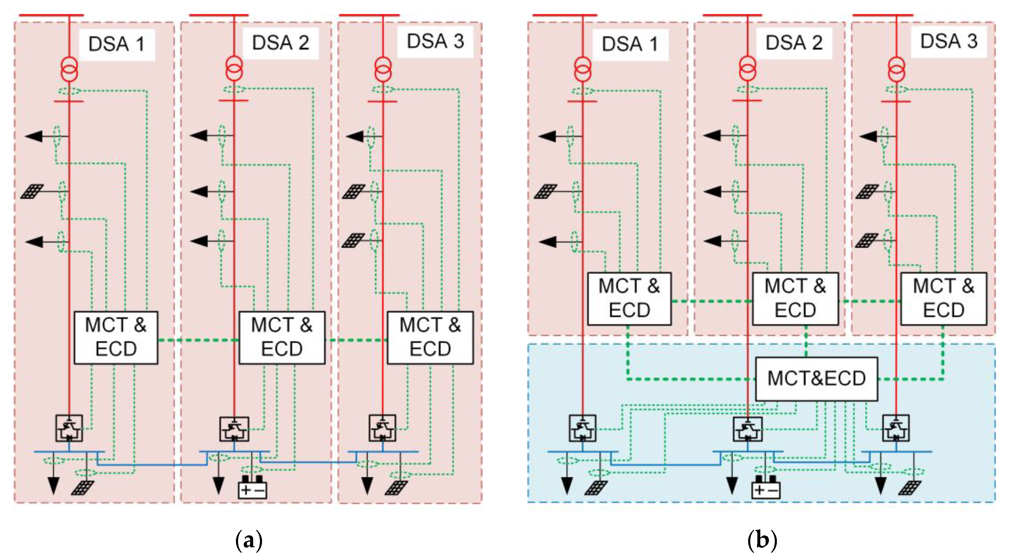
3.3. Decentralized Communication Architecture

The establishment and solution of the decentralized dispatch model are based on the result of network partitioning and so is the architecture for implementing decentralized dispatch. Two different network partitioning schemes have been proposed, each leading to a specific decentralized communication architecture as shown in Figure 3.

Architecture 1 involves grouping the converters, DC-side nodes, and their adjacent AC-DSAs into one area. The local measurements and control within this area are implemented by the originally existing MCT and ECD. Architecture 2, on the other hand, divides each AC-DSA and the entire DC side into different areas. The local data collection and control within each DSA utilize the existing MCT and ECD. Additionally, a separate MCT and ECD are introduced in the DC area to collect local data and control the converters and other controllable devices.

Architecture 1 is more efficient in terms of resource utilization and communication, as it saves one MCT and ECD. However, it cannot achieve the optimal selection of a control mode for the converter stations, which could further reduce the voltage deviation on the DC side. This limitation arises from the fact that ADMM cannot handle coupling constraints that involve binary variables. In the centralized dispatch model, the ability to optimally select the control mode of the converter stations is achieved by treating Equations (22) and (23) as constraints. However, when implementing decentralized dispatch using Architecture 1, Equation (23) becomes a coupling constraint among areas, and it involves binary variables, which may hinder convergence of the ADMM algorithm. Therefore, in Architecture 1, it becomes necessary to remove Equation (23), meaning that the control mode of the converter stations is not determined based on the control model but is predetermined. On the other hand, Architecture 2 avoids this issue. When implementing decentralized dispatch based on Architecture 2, Equation (23) is no longer a coupling constraint between areas but becomes a local constraint within the DC area. Therefore, the optimal selection of control modes for the converter stations can still be achieved.

To summarize, the advantages and disadvantages of Architecture 1 and Architecture 2 are as follows:

(1)

Architecture 1 has more efficient communication and lower investment costs. However, it cannot achieve the optimal selection of control modes for the converter stations. The voltage profile on the DC side can only reach suboptimal levels. This architecture is suitable for scenarios where the DC network is simple and there is tolerance for voltage deviations.

(2)

Architecture 2 allows for the optimal selection of control modes for the converter stations during decentralized dispatch implementation. It enables the optimal voltage profile on the DC side and can further reduce voltage deviations compared to Architecture 1. However, it requires an additional MCT and ECD, resulting in increased investment, and communication becomes relatively more complex. This architecture is suitable for scenarios with a more complex DC network and stricter voltage deviation requirements.

Indeed, it is worth noting that in both decentralized communication architectures, the computations are performed within each individual area, and only the exchange of coupling variable information is required between neighboring areas. This significantly reduces the computational and communication burden compared to the centralized dispatch scheme.

4. Case Study

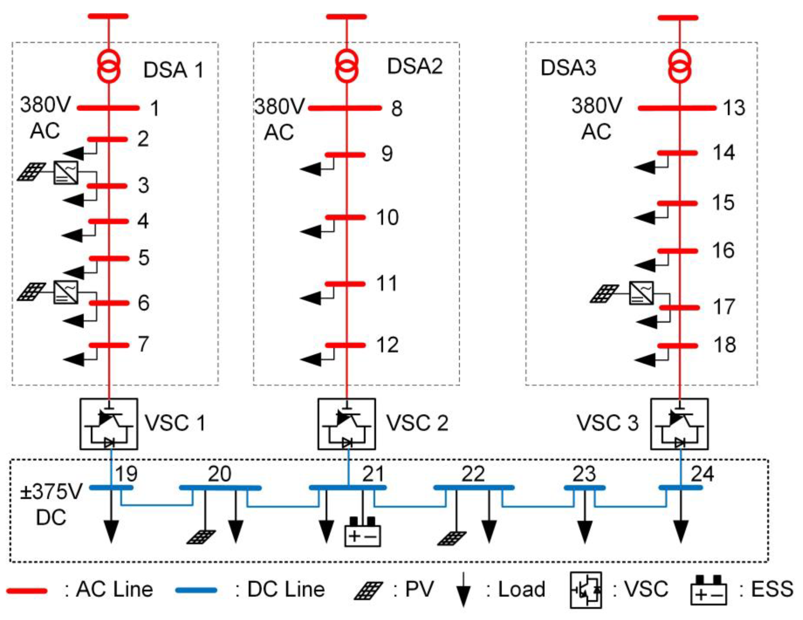
4.1. Case Setting

A case study is conducted on a 24–nodes AC–DC hybrid DN formed by flexible interconnected DSAs, as shown in Figure 4. The numbers 1–24 denote the node indexes. The parameter settings for this network are presented in

Table A1. Parameters of the AC–DC hybrid DN.

Parameter	Value
Rated voltage on the AC side	380 V
Rated voltage on the DC side	±375 V
Capacity of the transformer in DSA 1	400 kV·A
Capacity of the transformer in DSA 2	200 kV·A
Capacity of the transformer in DSA 3	315 kV·A
Capacity of the ESS at node 21	250 kW·h
Maximum charging/discharging power of the ESS	20 kW
Charging/discharging efficiency of the ESS	0.97
Capacity of the VSCs at node 7, 12, and 18	150 kV·A
Capacity of the PV at node 3	10 kV·A
Capacity of the PV at node 6	15 kV·A
Capacity of the PV at node 17	100 kV·A
Capacity of the PV at node 21 and 23	30 kV·A
Unit penalty price of PV output curtailment	2.5 CNY/(kW·h)

in Appendix A. The normalization curve of power output of PVs is shown in Figure A1, and the time-of-use (TOU) electricity price for purchasing electricity from the superior power grid is shown in Figure A2. For more detailed information, please refer to [23].

Three simulation scenarios were set up to validate the effectiveness of the proposed decentralized dispatch:

(1)

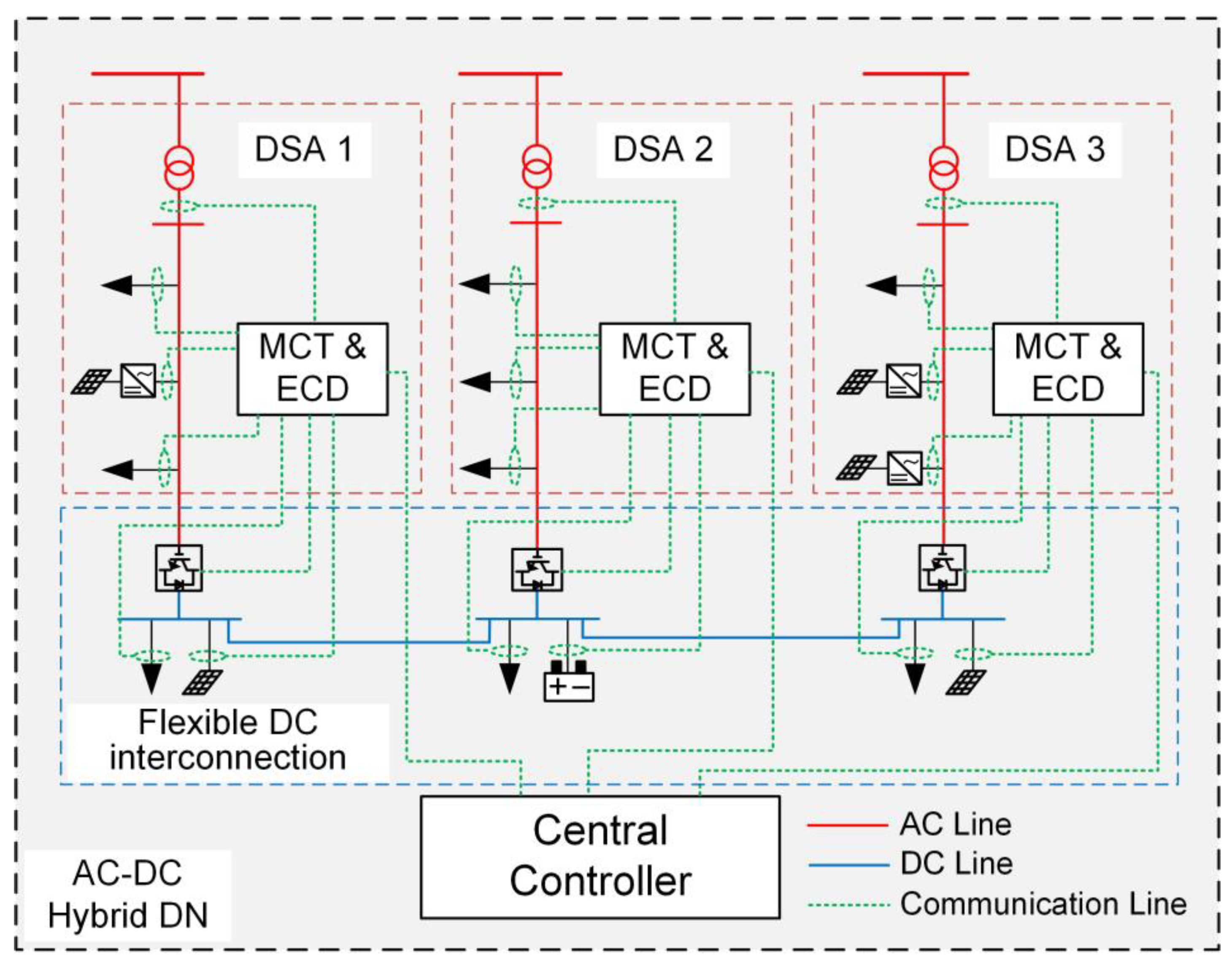
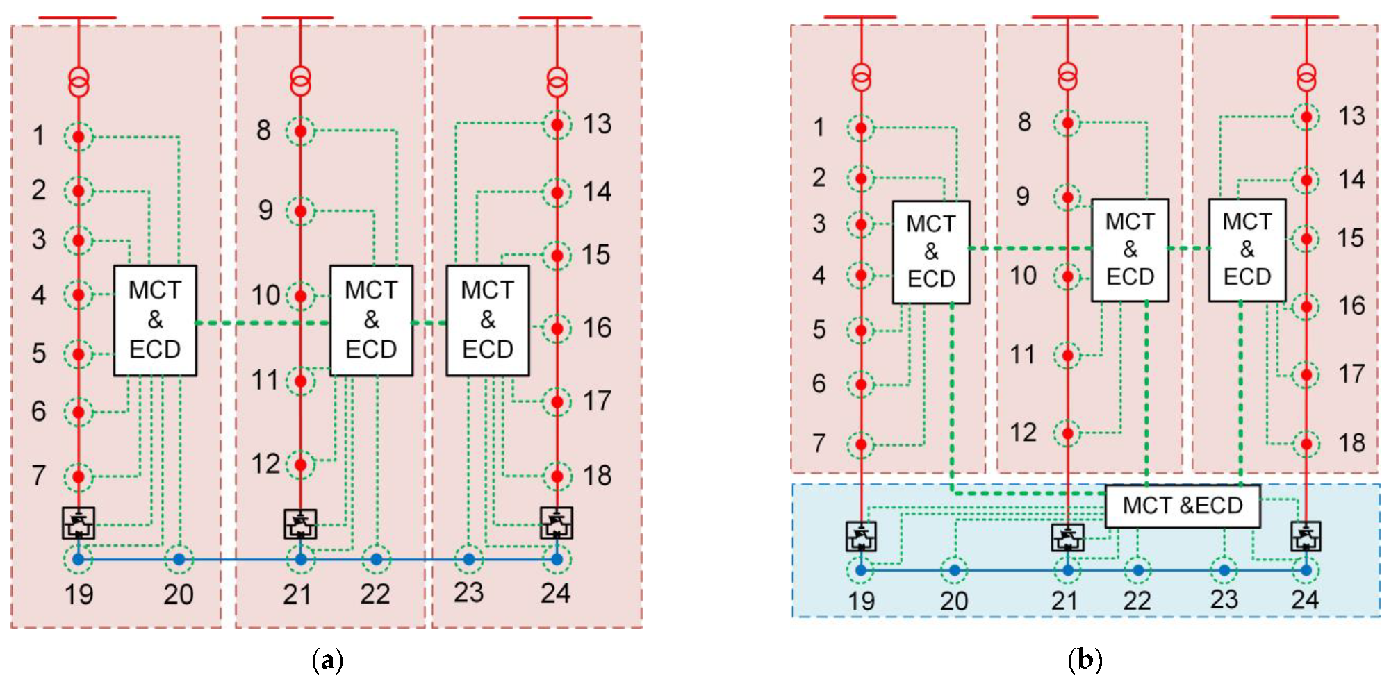
Scenario 1: The centralized optimal dispatch scheme is adopted. Based on the centralized communication architecture shown in Figure 1, the centralized optimal dispatch model described in Section 2 is solved to achieve the optimal operation state. The constraint incorporating the control modes of the converter stations is taken into consideration. Theoretically speaking, the dispatch results of Scenario 1 are optimal.

(2)

Scenario 2: The decentralized dispatch scheme corresponding to Architecture 1 is adopted, and the decentralized communication architecture is shown in Figure 5a. As mentioned earlier, due to the inability of ADMM to handle coupling constraints containing binary variables, the decentralized optimal dispatch model based on the network partitioning method used in Scenario 2 cannot achieve the optimal selection of the control modes for the converter stations. Instead, the control modes for each converter station are predefined before model solving. In this case study, VSC1 and VSC3 are defined to adopt the P-Q control mode, while VSC2 adopts the U_dc-Q control mode.

(3)

Scenario 3: The decentralized dispatch scheme corresponding to Architecture 2 is adopted, and the decentralized communication architecture is shown in Figure 5b. The network partitioning method used in Scenario 3 avoids treating the constraint (23) containing binary variables as a coupling constraint between areas. Therefore, the decentralized optimal dispatch model in Scenario 3 can incorporate constraint (23). Theoretically speaking, the decentralized optimal dispatch results of Scenario 3 should be the same as the centralized optimal dispatch results of Scenario 1.

4.2. Results and Discussion

4.2.1. Optimization Results of Objectives

The optimization results of objectives in the three scenarios are listed in

Table 2. Optimization results of three scenarios.

Objective	Scenario 1	Scenario 2	Scenario 3
f1	1.1765	1.5240	1.1328
f2	23.4260	23.7718	23.3947
f3	5775.9479	5799.2635	5780.4375
F	0.6041	0.6128	0.6038

.

Scenario 1 utilizes a centralized optimal dispatch method, which yields the optimal solution for the dispatch model. By comparing the optimization results of Scenario 2 and Scenario 3 with those of Scenario 1, it can be observed that the proposed decentralized optimal dispatch scheme achieves results close to the centralized optimal dispatch. This implies that optimal dispatch of flexible interconnected DSAs can be achieved without the need for a central controller, global communication, or heavy centralized computational burdens, which validates the effectiveness of the proposed method.

By comparing Scenario 2 and Scenario 3, it can be observed that different partitioning approaches result in slight deviations in the effectiveness of the decentralized optimal dispatch. The reason behind this lies in the partitioning approach used in Scenario 2 making the constraint expressing the selection of the converter station control model, that is, Equation (23), becoming a coupling constraint between areas. Since this constraint involves binary variables that cannot be handled by ADMM, Equation (23) is excluded when using the partitioning approach in Scenario 2. In other words, the control mode of the converter station is not considered in the decentralized optimal dispatch model for Scenario 2. On the other hand, the partitioning approach used in Scenario 3 avoids the issue of coupling constraints among areas for Equation (23), allowing for the inclusion of the converter station control mode in the model. Therefore, based on the partitioning approach used in Scenario 3, the decentralized optimal dispatch model is fully equivalent to the centralized optimal dispatch model. In addition, the optimal dispatch model based on Scenario 2 is a weakened version of Scenarios 1 and 3, with a smaller feasible domain. As a result, the optimization effectiveness of Scenario 2 is slightly inferior to that of Scenario 3, while the effectiveness of Scenario 3 is almost on par with Scenario 1.

Figure A3 and Figure A4 demonstrate the convergence process of residuals in Scenario 2 and Scenario 3. As the iteration progresses, the residuals rapidly decrease and reach convergence, which validates the feasibility of implementing decentralized solving of the optimal dispatch model using ADMM.

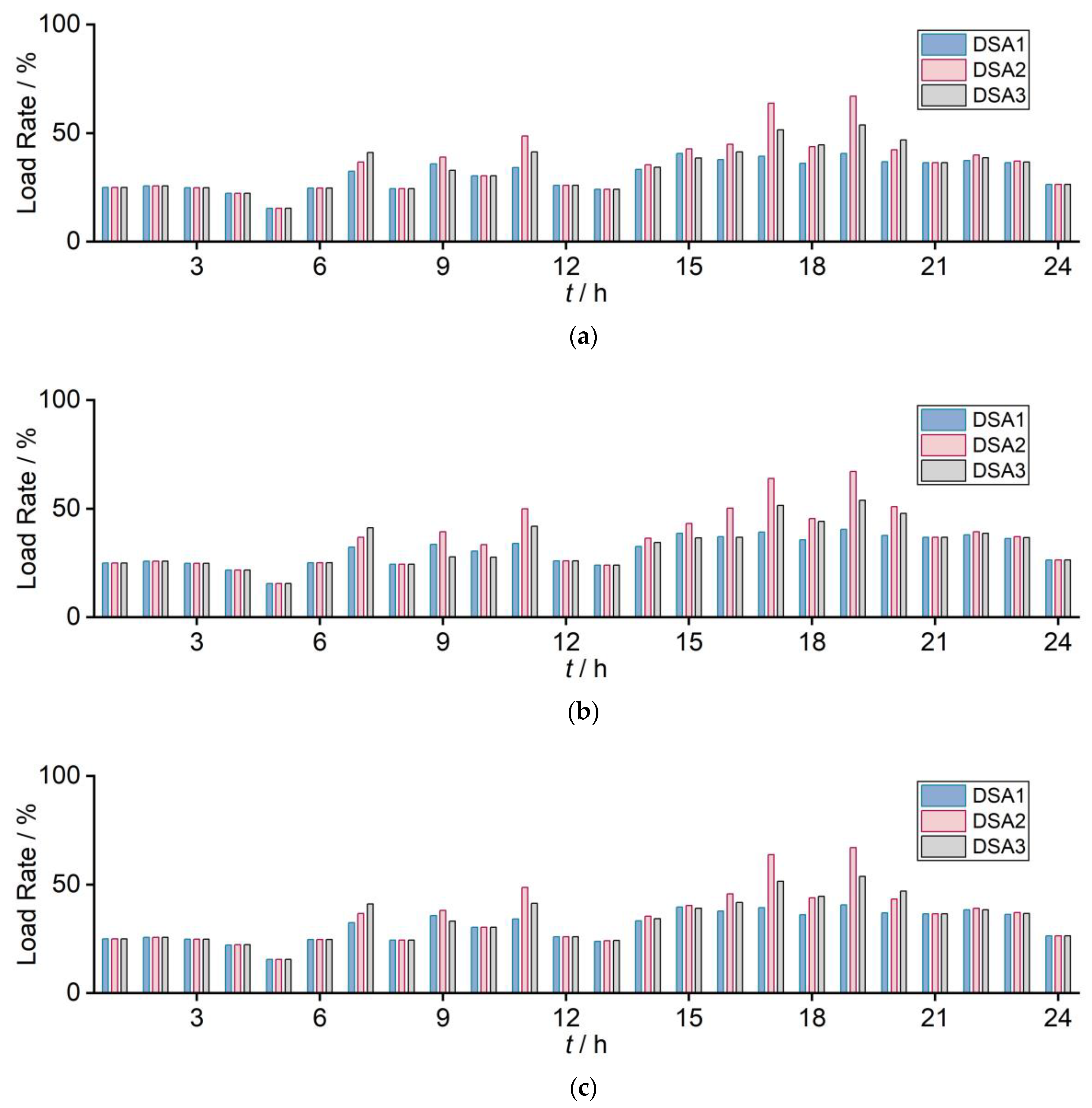
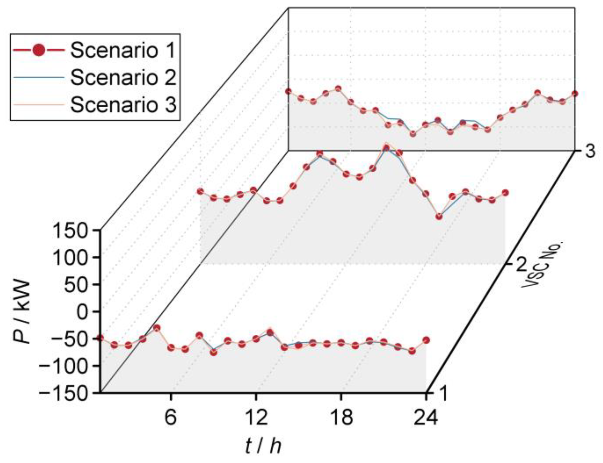
4.2.2. The Effectiveness of Load Rate Balancing in Three Scenarios

The load rates of the DSAs in the three scenarios are shown in Figure 6, and the active power transmitted by three VSCs is shown in Figure 7.

As shown in the Figure 6, the effectiveness of load rate balancing under the three scenarios is as follows:

(1)

Scenario 1: the centralized optimal dispatch scheme achieves excellent load balancing results.

(2)

Scenario 2: due to the exclusion of the converter station control model, resulting in a reduced feasible domain of the optimization model, the load balancing effectiveness is slightly compromised compared to Scenario 1 at some time points, such as t = 16 and 20.

(3)

Scenario 3: By employing the partitioning approach in this scenario, the exclusion of constraint (23) is avoided, resulting in the full equivalence of the decentralized optimization model and the centralized optimization model. As a result, the effectiveness of load rate balancing is nearly identical to that of Scenario 1.

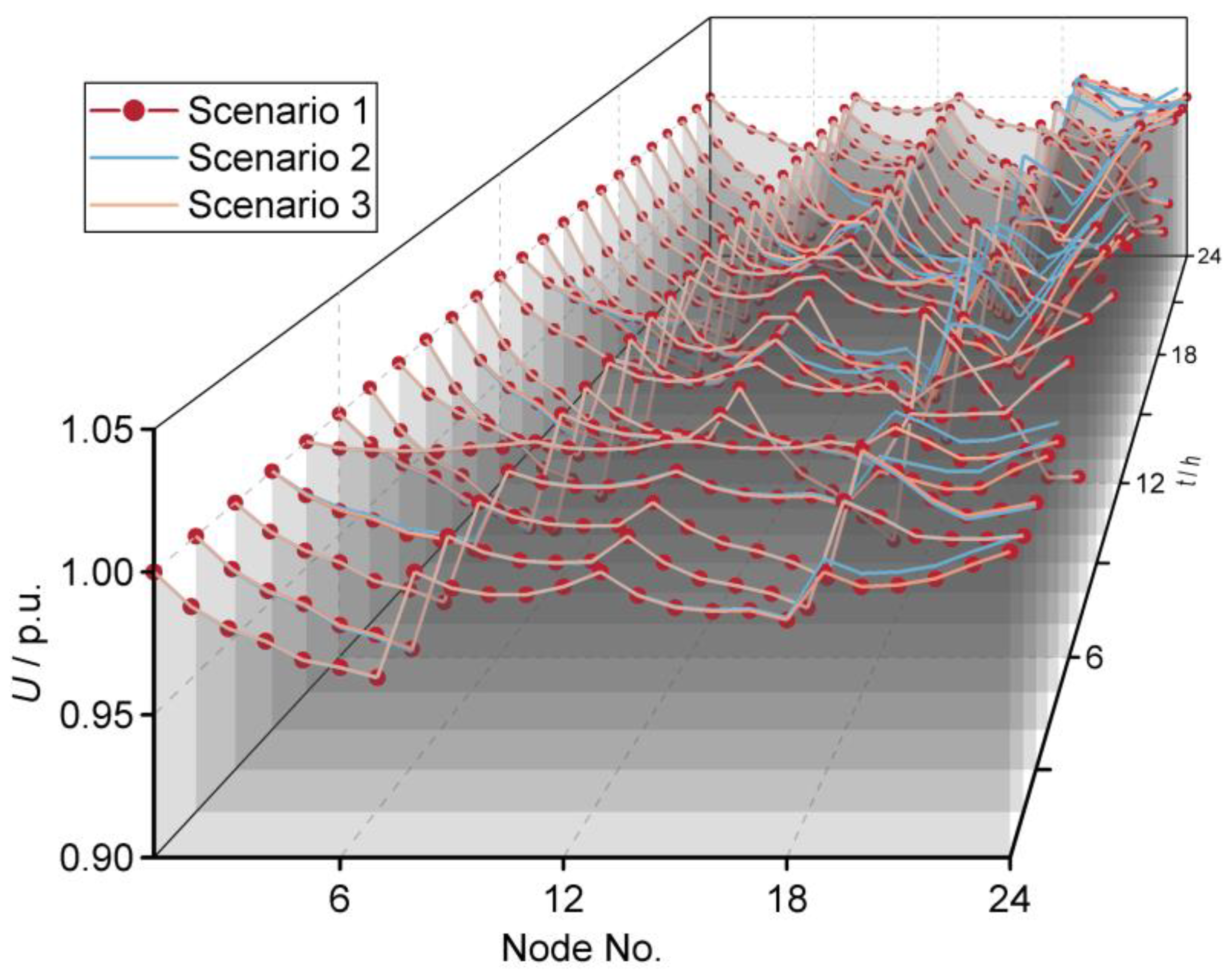
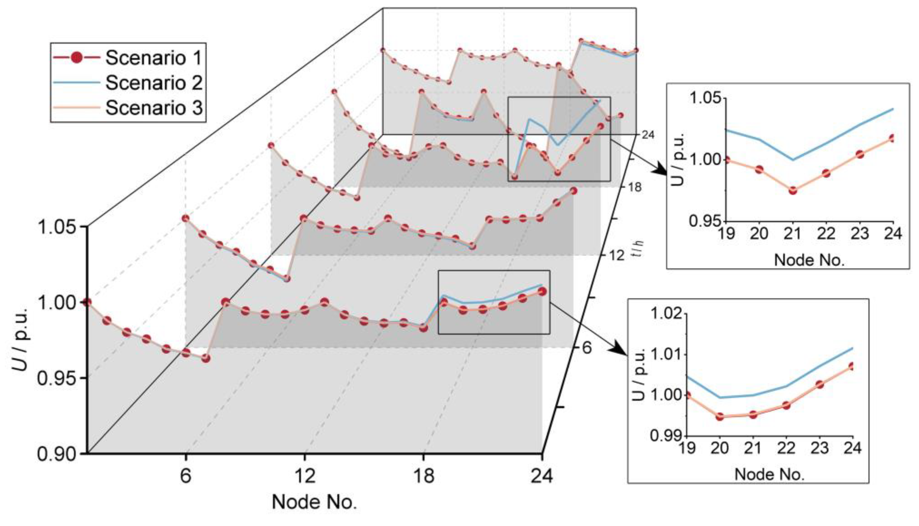
4.2.3. Voltage Profile Comparison among the Three Scenarios

The voltage profiles in the three scenarios are shown in Figure 8. To provide a clearer visualization, selected time points are chosen to display the voltage profiles. The voltage profile plots for all time points can be found in Figure A5.

In Figure 8, the x-axis label “Node No.” represents node numbers, where nodes 1 to 18 are AC-side nodes and nodes 19 to 24 are DC-side nodes. As shown in Figure 8, the voltage profiles of the AC-side nodes are nearly identical among the three scenarios. However, at some time points, such as t = 1 or 12, the DC-side node voltages in Scenario 2 exhibit higher deviations compared to Scenarios 1 and 3. On the other hand, the voltage profiles of the DC-side nodes in Scenario 1 and Scenario 3 are almost identical. This is because Scenario 2 did not incorporate the optimal selection of the control modes for the converter stations, which could further reduce the voltage deviation on the DC side, into the decentralized optimal dispatch model. Consequently, Scenario 2 exhibits slightly higher voltage deviations on the DC side compared to Scenarios 1 and 3. In Scenario 3, where the control modes of the converter stations are included in the decentralized dispatch model, the voltage profiles on the DC side are equivalent to those achieved by Scenario 1, which considers the control modes in the centralized dispatch model.

It is worth mentioning that adopting the decentralized dispatch scheme based on the result of network partitioning in Scenario 2 does not necessarily lead to a deterioration of the DC-side voltage. It simply means giving up the further optimization of the DC-side voltage profile by optimally selecting the combination of control modes for the converter stations.

4.2.4. Comprehensive Comparison of the Two Communication Architectures

In terms of effectiveness of load rate balancing, the decentralized dispatch based on Architecture 2 achieves results nearly identical to the centralized dispatch, while Architecture 1 only slightly lags behind the centralized dispatch at some time points. In terms of voltage profile optimization, Architecture 2 still achieves results nearly identical to the centralized dispatch scheme. Architecture 1 demonstrates the effectiveness comparable to that of the centralized dispatch scheme on the AC side but exhibits larger voltage deviations on the DC side.

In summary, both architectures can achieve the objectives of load rate balancing among DSAs and voltage profile optimization. However, Architecture 2 performs better than Architecture 1 in reducing voltage deviations on the DC side, and it is worth noting that compared to Architecture 2, Architecture 1 has lower costs and a simpler communication structure.

Therefore, Architecture 1 is recommended for scenarios where the DC-side voltage requirements are not as strict and the voltage is less prone to exceeding limits. On the other hand, Architecture 2 is recommended for scenarios with stringent DC-side voltage deviation requirements or where the voltage is more likely to exceed limits.

5. Conclusions

This paper proposes a decentralized dispatch scheme for an AC–DC hybrid DN formed by flexible interconnected DSAs, which achieves the goals of load rate balancing among DSAs and voltage profile optimization in a fully decentralized manner. Two communication architectures for implementing decentralized dispatch are introduced. Architecture 1 has advantages such as simpler communication architecture and lower investment. However, it can only achieve a suboptimal voltage profile on the DC side. Therefore, it is suitable for scenarios where the requirements for DC voltage deviation are not very strict or voltage violations are less likely to occur. On the other hand, based on Architecture 2, the decentralized dispatch scheme can achieve results that are nearly identical to the centralized dispatch scheme considering the optimal selection of the control modes of the converter stations. It can achieve the optimal voltage profile on the DC side. However, compared to Architecture 1, the communication architecture of Architecture 2 is more complex and requires higher investment. So, it is suitable for scenarios with strict requirements for DC voltage deviation or where voltage violations are more likely to occur.

Future work will further incorporate the consideration of the stochastic nature of load demand and DG outputs into the model.

References

- Liu, W.; Lü, Z.; Liu, H. An overview of morphological development and operation control technology of power electronics dominated distribution area. Proc. CSEE 2023, in press. [Google Scholar]
- Lin, J.; Wan, C.; Song, Y.H.; Huang, R.L.; Chen, X.S.; Guo, W.F.; Zong, Y.; Shi, Y. Situation awareness of active distribution network: Roadmap, technologies, and bottlenecks. CSEE J. Power Energy Syst. 2016, 2, 35–42. [Google Scholar] [CrossRef]
- Xu, W.T.; Zeng, S.M.; Du, X.D.; Zhao, J.L.; He, Y.L.; Wu, X.W. Reliability of active distribution network considering uncertainty of distribution generation and load. Electronics 2023, 12, 1363. [Google Scholar] [CrossRef]
- Wang, J.X.; Qin, J.J.; Zhong, H.W.; Rajagopal, R.; Xia, Q.; Kang, C.Q. Reliability value of distributed solar plus storage systems amidst rare weather events. IEEE Trans. Smart Grid 2019, 10, 4476–4486. [Google Scholar] [CrossRef]
- Walling, R.A.; Saint, R.; Dugan, R.C.; Burke, J.; Kojovic, L.A. Summary of distributed resources impact on power delivery systems. IEEE Trans. Power Deliv. 2008, 23, 1636–1644. [Google Scholar] [CrossRef]
- O’Shaughnessy, E.; Cruce, J.R.; Xu, K.F. Too much of a good thing? Global trends in the curtailment of solar PV. Sol. Energy 2020, 208, 1068–1077. [Google Scholar] [CrossRef] [PubMed]
- Xu, Y.; Liu, H.; Xiong, X.; Ji, Y.; Shao, Y.; Zhang, H.; Sun, L.; Wu, M. Key technologies and development modes of flexible interconnection of low-voltage distribution station area. Proc. CSEE 2022, 42, 3986–4001. [Google Scholar]
- Liu, H.; Dong, X.; Xiong, X.; Xu, Y. Energy interconnection and energy microcirculation system of terminal power grid based on low-voltage flexible DC. Autom. Electr. Power Syst. 2023, 47, 40–47. [Google Scholar]
- Xie, M.; Zhang, S.; Li, Y.; Huang, Y.; Liu, M. An optimal dispatch model for AC/DC low-voltage distribution network based on multi-mode flexible interconnection. Autom. Electr. Power Syst. 2023, 47, 79–89. [Google Scholar]
- Cao, W.; Wu, J.; Jenkins, N.; Wang, C.; Green, T. Benefits analysis of soft open points for electrical distribution network operation. Appl. Energy 2016, 165, 36–47. [Google Scholar] [CrossRef] [Green Version]
- Dastgeer, F.; Gelani, H.E.; Anees, H.M.; Paracha, Z.J.; Kalam, A. Analyses of efficiency/energy-savings of DC power distribution systems/microgrids: Past, present and future. Int. J. Electr. Power Energy Syst. 2019, 104, 89–100. [Google Scholar] [CrossRef]
- Flexible Urban Networks: Low Voltage Project Progress Report; UK Power Networks: London, UK, 2016.
- Huang, Z. Research on Operation and Control of Zhuhai Three Terminal Flexible DC Distribution Network. Master’s Thesis, South China University of Technology, Guangzhou, China, 2021. [Google Scholar]
- Cao, W. Soft Open Points for the Operation of Medium Voltage Distribution Networks. Ph. D. Thesis, Cardiff University, Wales, UK, 2015. [Google Scholar]
- Zhang, T.; Mu, Y.F.; Jia, H.J.; Wang, X.Y.; Pu, T.J. Successive MISOCP algorithm for islanded distribution networks with soft open points. CSEE J. Power Energy Syst. 2023, 9, 209–220. [Google Scholar]
- Rezaeian-Marjani, S.; Galvani, S.; Talavat, V. A generalized probabilistic multi-objective method for optimal allocation of soft open point (SOP) in distribution networks. IET Renew. Power Gener. 2022, 16, 1046–1072. [Google Scholar] [CrossRef]
- Wang, J.; Wang, W.Q.; Yuan, Z. Operation optimization adapting to active distribution networks under three-phase unbalanced conditions: Parametric linear relaxation programming. IEEE Syst. J. 2023, in press. [Google Scholar] [CrossRef]
- Sarantakos, I.; Peker, M.; Zografou-Barredo, N.M.; Deakin, M.; Patsios, C.; Sayfutdinov, T.; Taylor, P.C.; Greenwood, D. A Robust mixed-integer convex model for optimal scheduling of integrated energy storage-soft open point devices. IEEE Trans. Smart Grid 2022, 13, 4072–4087. [Google Scholar] [CrossRef]
- Ji, H.R.; Wang, C.S.; Li, P.; Zhao, J.L.; Song, G.Y.; Ding, F.; Wu, J.Z. An enhanced SOCP-based method for feeder load balancing using the multi-terminal soft open point in active distribution networks. Appl. Energy 2017, 208, 986–995. [Google Scholar] [CrossRef]
- Wang, X.; Chen, R.; Ge, J.; Cao, T.; Wang, F.; Mo, X. Application of AC/DC distribution network technology based on flexible substation in regional energy internet. In Proceedings of the 2019 IEEE Innovative Smart Grid Technologies-Asia (ISGT Asia), Chengdu, China, 21–24 May 2019; pp. 4340–4345. [Google Scholar]
- Alhasnawi, B.N.; Jasim, B.H.; Mansoor, R.; Alhasnawi, A.N.; Rahman, Z.A.S.A.; Haes Alhelou, H.; Guerrero, J.M.; Dakhil, A.M.; Siano, P. A new internet of things based optimization scheme of residential demand side management system. IET Renew. Power Gener. 2022, 16, 1992–2006. [Google Scholar] [CrossRef]
- Corinaldesi, C.; Fleischhacker, A.; Lang, L.; Radl, J.; Schwabeneder, D.; Lettner, G. European case studies for impact of market-driven flexibility management in distribution systems. In Proceedings of the 2019 IEEE International Conference on Communications, Control, and Computing Technologies for Smart Grids (SmartGridComm), Beijing, China, 21–23 October 2019; pp. 1–6. [Google Scholar]
- Tang, X.; Qin, L.; Yang, Z.C.; He, X.L.; Min, H.D.; Zhou, S.H.; Liu, K.P. Optimal Scheduling of AC–DC hybrid distribution network considering the control mode of a converter station. Sustainability 2023, 15, 8715. [Google Scholar] [CrossRef]
- Yang, L.; Sun, Q.; Zhang, N.; Li, Y. Indirect multi-energy transactions of energy internet with deep reinforcement learning approach. IEEE Trans. Power Syst. 2022, 37, 4067–4077. [Google Scholar] [CrossRef]
- Liu, H.; Wu, W. Federated reinforcement learning for decentralized voltage control in distribution networks. IEEE Trans. Smart Grid 2022, 13, 3840–3843. [Google Scholar] [CrossRef]
- Kou, P.; Liang, D.; Gao, R.; Liu, Y.; Gao, L. Decentralized model predictive control of hybrid distribution transformers for voltage regulation in active distribution networks. IEEE Trans. Sustain. Energy 2020, 11, 2189–2200. [Google Scholar] [CrossRef]
- Dong, L.; Zhang, T.; Pu, T.; Chen, N.; Sun, Y. A decentralized optimal operation of AC/DC hybrid microgrids equipped with power electronic transformer. IEEE Access 2019, 7, 157946–157959. [Google Scholar] [CrossRef]
- Erseghe, T. Distributed optimal power flow using ADMM. IEEE Trans. Power Syst. 2014, 29, 2370–2380. [Google Scholar] [CrossRef]
- Dorostkar-Ghamsari, M.R.; Fotuhi-Firuzabad, M.; Lehtonen, M.; Safdarian, A. Value of distribution network reconfiguration in presence of renewable energy resources. IEEE Trans. Power Syst. 2016, 31, 1879–1888. [Google Scholar] [CrossRef]
- Su, Y.; Teh, J. Two-stage optimal dispatching of AC/DC hybrid active distribution systems considering network flexibility. J. Mod. Power Syst. Clean Energy 2023, 11, 52–65. [Google Scholar] [CrossRef]
- Li, Z.W.; Xie, X.L.; Cheng, Z.P.; Zhi, C.Y.; Si, J.K. A novel two-stage energy management of hybrid AC/DC microgrid considering frequency security constraints. Int. J. Electr. Power Energy Syst. 2023, 146, 12. [Google Scholar] [CrossRef]
- Boyd, S.; Parikh, N.; Chu, E.; Peleato, B.; Eckstein, J. Distributed optimization and statistical learning via the alternating direction method of multipliers. Found. Trends Mach. Learn. 2011, 3, 1–122. [Google Scholar] [CrossRef]