

Optimal Green Input Level for a Capital-Constrained Supply Chain Considering Disruption Risk

School of Economics, Fujian Normal University, Fuzhou 350108, China
*
Author to whom correspondence should be addressed.
Sustainability 2023, 15(15), 12095; https://doi.org/10.3390/su151512095
Submission received: 10 June 2023
/
Revised: 31 July 2023
/
Accepted: 3 August 2023
/
Published: 7 August 2023
(This article belongs to the Special Issue Green Supply Chain and Sustainable Economic Development)
Abstract
:Under increasingly stringent environmental regulations, inadequate green input levels from manufacturers may lead to substandard emissions and production shutdown, which further results in the disruption risk of the supply chain. This work investigates a green supply chain (GSC) consisting of one environmentally regulated manufacturer and one capital-constrained retailer who faces stochastic market demand. The manufacturer needs to make decisions on the green input level, which is related to the investment cost as well as supply disruption risk. The retailer has to determine product order quantities and financing decisions. We derive the operational equilibriums for the GSC system under three scenarios: no financing, trade credit financing (TCF), and bank credit financing (BCF), and recommend the optimal financial selection for the retailer via the comparison of three financial modes. The analytical and numerical results reveal that the manufacturer should improve the green input level within the financial capability to enhance the sustainable operation level of the supply chain. In addition, we find that the capital-constrained retailer will choose financing, since either BCF or TCF will result in a higher profit than no financing. Moreover, we obtain the threshold of green input level, with which we can decide whether to choose TCF or BCF under the given corresponding parameters.
1. Introduction
In order to combat global warming and promote sustainable development, the international community has reached several important climate agreements to control carbon emissions in recent decades, such as the Kyoto Protocol, the Paris Agreement, and the Glasgow Climate Convention. At the beginning of 2023, there were over 187 countries that had submitted Voluntary National Reviews to the United Nations [1], which report the progress and policy efforts of their sustainable development goals, and many of them have introduced a series of environmental control regulations [2]. For example, Brazil has promoted economical irrigation systems to reduce greenhouse gas emissions from livestock rearing, with the aim of achieving carbon neutrality by 2050. Meanwhile, as the concept of sustainability becomes increasingly popular, environmentally friendly products are becoming more relevant to consumers’ demand preferences [3]. The individuality and diversification of consumer demand also deepen the demand uncertainty [4,5].
Under the dual pressure of government environmental regulations and market demands, more and more companies are actively investing in cleaner production and pursuing green development [4]. In the supply chains consisting of manufacturers and retailers, inadequate green input levels from manufacturers may lead to substandard emissions and supply disruption. For example, more than thirty regions in China shut down a number of enterprises due to pollution issues in January 2023. The shutdown not only affects the manufacturer’s own operations and reputation, but also deteriorates the retailer’s supply stability and expected revenues. To better pass environmental inspections, manufacturers should invest more in cleaner production, which incurs higher production costs and ultimately leads to lower profit. Therefore, it is of great significance to investigate the optimal green input level of manufacturers for supply chain management, especially taking the green input level as a decision variable related to the supply disruption risk [6].
Meanwhile, in manufacturer-centric supply chains, most retailers are small- and medium-sized enterprises (SMEs), which often suffer from the challenge of insufficient working capital for operations [7]. When retailers face funding shortage, they can reduce order quantity to shrink business volume or seek support from banks according to the local green credit policies and SME support policies, which is known as bank credit financing (BCF) [4,8]; in addition, upstream manufacturers may also be willing to provide flexible payment options to relieve retailers’ financial pressure and ensure the realization of order requirements, which is known as trade credit financing (TCF) [7]. Different financing modes correspond to different trade contracts, which leads to different supply chain capital efficiency and equilibrium [9].
In a two-echelon supply chain consisting of a single manufacturer and a capital-constrained retailer, when the green input level is considered as a decision variable related to disruption risk, and the market demand is stochastic, the following new research problems are intriguing and worthy of being explored:
- How different would the game problem of a two-echelon supply chain be when considering the decision of green input level?
- With different financing modes, i.e., BCF and TCF, how does the retailer determine the order quantity to maximize profit?
- How does the manufacturer decide the green input level to achieve the optimal profit with the given order quantity of the retailer?
- How will the retailer select the financing mode? Does the option of financing help reduce the risk of supply disruption compared to no financing?
To answer the above questions, we investigate a green supply chain consisting of one environmentally regulated manufacturer and one capital-constrained retailer who faces stochastic market demand. The manufacturer needs to make decisions on the green input level, which is related to the risk of supply disruption and investment cost. The retailer needs to capture product order quantities and financial decisions for greater profit. We deduce the optimal operational decisions of manufacturer and retailer under BCF and TCF modes, respectively, using the newsvendor model under environmental regulation. The scenario of no financing is also analyzed and regarded as a benchmark model. We employ the Stackelberg game rule and acquire the optimal decisions of the retailer and the manufacturer by means of a backward induction method, where the manufacturer is the leader, and the retailer is the follower. The results suggest that retailers with limited capital will be willing to choose financing, since either BCF or TCF results in higher profit for the retailer. By further comparing the financing models, the threshold of optimal financing mode selection is recommended for the retailer based on different demand functions and other parameters.
This work contributes to the literature in three aspects. First, we establish a new Stackelberg game model for a two-echelon supply chain problem, which involves financial constraint, green input level, and stochastic market demand, and the green input level is considered as a decision variable related to supply disruption risk. Second, we derive the equilibriums of the supply chain members under no financing, BCF, and TCF scenarios and further analyze the interactions between decision-making variables. Third, a financing mode recommendation is given based on the comparison of different financing models with deduced green input thresholds. The retailer will prefer bank credit financing if the risk of supply disruption under BCF is low relative to TCF. Finally, we verified and visualized the conclusions with numerical examples.
The remainder of this paper is organized as follows. Section 2 provides a systematic review of the relevant literature, followed by the understudied problem description and hypotheses statements in Section 3. Section 4 presents the deduction of optimal decisions for the supply chain members under the no financing, TCF, and BCF scenarios, as well as the financing mode comparison. Section 5 shows the numerical simulations and sensitivity analysis. Finally, we summarize this work and point out the future research directions.
2. Literature Review
Our work focuses on the optimal green input level for capital-constrained supply chains considering disruption risk under different financing modes with stochastic market demand. Thus, the relevant literature mainly includes green supply chain management (GSCM), supply chain financing, and supply chain management considering disruption risk.
2.1. Green Supply Chain Management
There is a large body of literature on green supply chain management from recent decades. It can mainly be divided into the following categories: empirical studies on impact factors or performance outcomes of GSCM practice [10], GSCM operation research studies using mathematical modeling or optimization algorithms [11], and game behavior and tactical decisions of GSC members [12,13]. The last stream is related to our work, where many different elements have been considered by scholars when constructing game models, such as government subsidies, consumer preferences, marketing efforts, recycling strategy, environmental considerations, etc. Next, we focus on reviewing the works of green supply chain management, considering the environmental regulation or impact closely related to this study.
Some scholars focused on exploring the effects of different environmental regulation policies. Chen and Sheu [14] found that proper environmental regulation pricing strategies can promote rational manufacturers to improve their product recyclability in a competitive market. Rosič and Jammernegg [15] investigated the optimal order quantity of the dual-sourcing model by considering the environmental regulations for transport, and found that emission trading is more reasonable than emission tax. Liu et al. [16] found that the supply chain players with superior eco-friendly operations benefit from an increase in consumers’ environmental awareness. Chen et al. [17] analyzed the manufacturing and remanufacturing decisions of a monopoly manufacturer under environmental regulations, and verified that the government’s supervision of carbon trading prices is important to reduce the environmental impact. Fang and Xu [7] investigated that the introduction of a carbon tariff does not necessarily reduce global carbon emissions under certain conditions. Wang et al. [18] studied a couple of incentive mechanisms for collaboratively enhancing the green degree of products in a green supply chain system. Yu et al. [19] explored the carbon emission efforts and pricing decisions for green supply chain members under carbon taxation. Bai et al. [20] examined the effect of financial incentives with emission reduction constraints on the supply chain’s operational decisions and environmental performance. The above works demonstrate that it is necessary for supply chain members to actively increase green input levels under environmental regulation policies.
Many scholars studied the optimal operational decisions of supply chain members under a given environmental regulation policy. Du et al. [21] proved that the emission-dependent manufacturer and the emission permit supplier under a cap-and-trade policy can obtain more profit by coordinating the supply chain under certain circumstances. Later, Du et al. [22] extended the previous work by further considering consumer’s low-carbon premium and found the conditions under which low-carbon production is profitable. Mondal and Giri [23] developed a centralized policy and three decentralized policies for a closed-loop green supply chain under a cap-and-trade policy and government intervention. Gao et al. [24] focused on a dual-channel supply chain management problem where the manufacturer encountered the restriction of green standards and proposed a two-part tariff contract for the supply chain players. Jian et al. [25] investigated the optimal strategies of green closed-loop supply chain members under centralized decision making and decentralized decision making. Liu et al. [26] established a game model to analyze the optimal operating strategy and utility of the agricultural supply chain when investing in emission reduction. Yang et al. [27] have studied the optimal pricing and sourcing tactics of supply chains under supply uncertainty.
From the summarization of the above works, it can be concluded that most of the previous studies mainly focused on deciding optimal order quantity or product price, and few works considered green input level as a decision variable. As environmental regulations become more and more stringent, it is important to optimize green input levels for supply chain members to promote economic and sustainable operations. This work draws on Christopher et al. [6], who pioneered the combination of effort cost, sales expectation, and expected profit functions. We expand their core idea and combine green input levels and disruption risk to examine the operational and financing decisions for capital-constrained green supply chains under environmental regulation.
2.2. Supply Chain Finance
Supply chain financing has attracted wide attention from academic and industrial fields because of the difficulties and expensive costs for small and medium-sized enterprises to solve their capital shortage problems through traditional financing channels [8,28,29,30]. For example, Wuttke et al. [31] showed that supply chain finance management can strengthen the buying firm’s working capital position. Kouvelis and Zhao [32] proposed the applicable conditions of revenue-sharing financing in the supply chain. Chen et al. [33] suggested reverse trade credit financing to assist the capital-constrained manufacturer in production. Shi et al. [34] investigated a capital-constrained Newsvendor problem and found that all the supply chain members can benefit when the buyback price coefficient fell within a “Pareto Zone”. Jin et al. [35] showed that supplier intermediate financing can help to improve the supply chain members’ profits. Zhang and Chen [36] demonstrated the profitable condition of trade credit financing strategies in capital-constrained supply chains, thus achieving a win–win situation for the participants. Meanwhile, Huang et al. [28] conducted a comparison of supply chain financing with traditional bank credit financing and suggested their own applicable conditions.
Furthermore, increasing research interest is devoted to green supply chain financing. Wu et al. [4] studied the optimal operational decisions of supply chains in a carbon abatement environment under TCF, BCF, and blended financing, respectively. Zou et al. [37] investigated the operational strategy and financing decision of a two-echelon supply chain with uncertain product yield under a cap-and-trade carbon emission scheme and found that the financing decision depends on the manufacturer’s initial working capital. Fang and Xu [7] derived an equilibrium for a green supply chain financing system under scenarios of green credit financing and mixed financing, respectively, and verified the manufacturer’s willingness to conduct green investment as well as the benefit of the retailer’s partial prepayment. Luo et al. [5] studied the optimal procurement decision of a capital-constrained green supply chain and put forward the preferred selection between supplier financing and bank financing. Sun et al. [38] investigated the optimal production and financing decision of a capital-constrained closed-loop supply chain and proposed the critical conditions of optimal financing strategies for the original equipment manufacturer. Shi et al. [39] focused on a low-carbon product supply chain and explored how a capital-constrained supplier made decisions on production, carbon abatement investment, and insufficient emission permit purchase.
To sum up, previous studies have proposed abundant financing modes and operational decisions for supply chain members. However, the disruption risk associated with green input level has not been discussed in capital-constrained supply chains. This work hopes to explore the topic, drawing on both the trade credit financing mode and traditional bank financing mode in the literature.
2.3. Supply Chain Management Considering Disruption Risk
Supply chain disruptions, which refer to the disruption of the normal materials and goods flow within a supply chain [40], have attracted many scholars’ research interests in recent decades due to the increasing occurrence of uncertain and vulnerable events, such as unpredictable disasters, terrorist acts, natural calamities, etc. Li et al. [41] examined the operational decisions of a retailer with multiple supply sources to protect against the supply disruption risk from upstream manufacturers. Torabi et al. [42] investigated some proactive strategies to enhance the response capability of supply chain disruption, such as suppliers’ business plans and contracting with backup suppliers. Yu et al. [43] found the impacts of supply disruption risks on the choice between single and dual sourcing methods. Gupta et al. [44] studied the impacts of exogenous contingencies on the operational decisions of downstream members of the supply chain and found that the actual supply status of unreliable suppliers and the timing of competitors’ purchases were critical to the profitability of the buyer. Hu et al. [45] examine supply chain design issues and risk mitigation strategies under the disruption risk related to uncertainty in production levels.
However, the above articles mainly focused on the supply chain disruption risk resulting from external uncontrollable or unplanned events, while the production shutdown risk under given stringent environmental regulations is closely related to the efforts of cleaner production. In other words, manufacturers can influence the probability of supply disruptions by determining the green input level. This paper enriches the above research area with an in-depth discussion of supply disruption events in relation to their own level of effort.
To more clearly demonstrate the differences between this work and existing studies, we summarize the closely relevant literature in Table 1. From the table, we can see that previous research mainly considers green supply chains and supply chain financing, and these studies focus on optimal decisions for green supply chain operations or financing decisions. However, the impacts of green input level and supply stability under environmental regulation issues are rarely simultaneously considered. In this paper, we consider both the operational and financial decisions of the retailer, as well as the optimal green input level related to the supply disruption risk of the manufacturer in a green supply chain. Furthermore, compared to many studies that assumed the demand as a deterministic function of price or greenness [46], this work considers stochastic demand. We contribute to the literature by providing a new operational perspective on green supply chain financing at the level of risk management. Meanwhile, the close relationship between variables such as green input and ordering volume may provide new insights for policymakers.
3. Model Description and Hypothesis
The two-echelon supply chain considered in this paper consists of an environmental regulated manufacturer and a capital-constrained retailer. On the side of the retailer, the order quantity to the manufacturer is determined according to the stochastic market demand and its expected profit function. To cope with the capital shortage, the retailer can choose TCF or BCF for financing in line with different commitment contracts.
The manufacturer produces the goods at unit cost , and supplies to the retailer at a wholesale price or following BCF or TCF financing commitments, respectively. It is assumed that , since the manufacturer provides financing support and shares the retailer’s final sales proceeds under TCF. The input level of cleaner production to be determined is denoted by , , which indicates the probability that the manufacturer can keep sustainable production; conversely, expresses the risk of production interruption [6,49]. Based on the law of diminishing marginal utility, the investment cost of carbon emission reduction is [4,5], where is a constant called the cleaner production cost parameter.
The retailer determines order quantity q to the manufacturer according to the stochastic market demand D. Its probability density function is denoted by and its cumulative distribution function by . Following the work of [3], it is assumed that the general failure rate and the hazard rate are increasing with . The final sales volume achieved will not exceed either D or , i.e., will equal to . To pursue higher profit, the retailer prefers larger , for which the initial working capital is not sufficient, i.e., .
The retail price p of the product remains unchanged during the sales cycle. Since the possibility of the supply chain remaining sustainable is t, the expected average retail price can be calculated as . To avoid triviality and ensure profitable trading, it is assumed that [50]. The expected income of the retailer is . By normalizing the retail price to 1 [51], it can be obtained that .
Before the start of the selling season, the manufacturer establishes a general contract (, , , , ) with the retailer, where is the loan interest rate of the bank under BCF, is the lowest level of carbon emission reduction to avoid credit risk, and represents the revenue-sharing ratio under TCF. Then, the retailer decides the order quantity to the manufacturer and selects the financing mode. Subsequently, the manufacturer decides on the investment in cleaner production and starts production.
When the retailer chooses TCF, he will pay from his initial working capital at the beginning of the period, and transfer proportion of revenue to the manufacturer as a TCF fee at the end of the period.
When the retailer chooses BCF, the retailer gets a loan from the bank and pays to the manufacturer in the beginning. After the realization of market demand, the retailer repays the loan with residual revenue. If the residual revenue is insufficient to repay, the retailer goes bankrupt, and the bank obtains the residual value.
The sequence of events can be summed up in Figure 1.
For the problem, we consider establishing a Stackelberg Leadership Model with the manufacturer as the core enterprise. To facilitate the model expression, the notations are listed in Table 2.
Without loss of generality, the following assumptions are given. (1) Based on the above statement, the relationship of the parameters satisfies [51]. (2) A single-period product market is considered. (3) The capital market is perfectly competitive, where the expected profit of the bank is zero. Thus, the time value of the capital can be ignored [8,52]. (4) The manufacturer and the retailer are risk-neutral and perfectly rational.
4. Model Analysis
On the basis of the above statements, we will analyze three kinds of financing modes and discuss their equilibrium decisions in this section.
4.1. No Financing: The Benchmark
To facilitate the comparison of financing benefits, we first discuss the no-financing situation. The wholesale price is the same as that in the BCF mode since the manufacturer does not participate in the retailer’s financing. When the initial working capital of the retailer , the retailer faces a capital shortage. Now, we discuss the equilibrium strategies without financing.
The expected income of the retailer is , and he should pay to the manufacturer for the production. The expected profit of the retailer is
Proposition 1.
Lacking enough working capital, is the optimal equilibrium for the retailer without financing; satisfies the following equations:
Proof of Proposition 1.
Since , is concave with . Then, according to , we can obtain the retailer’s optimal quantity , which satisfies the following equation: . When , is a monotone increasing function of . Because , the retailer will pay all of his capital. Thus, the optimal order quantity . □
Proposition 1 indicates that when there is no financing, the retailer should pay all of his capital to the manufacturer and obtain the quantity of the corresponding goods to obtain optimal profit.
As mentioned previously, it is assumed that the market information can be observed perfectly. It is known that the manufacturer can receive the capital from the retailer while needing to produce numbers of products at unit production cost c and pay for carbon reduction input . Thus, the expected profit function of the manufacturer is as follows:
Proposition 2.
In the scenario of no financing, is the optimal equilibrium for the manufacturer and .
Proof of Proposition 2.
Since and , is a monotonous decrease function of , the optimal input level of cleaner production . □
Proposition 2 illustrates that under the no-financing mode, the manufacturer will choose to invest the minimum green input level to optimize his profit. Moreover, we can find that the manufacturer’s profit function decreases with t, which would be detrimental to reducing the supply disruption risk and further be adverse to protecting the retailer’s profit.
4.2. Trade Credit Financing
The retailer’s restricted working capital not only affects its own revenue, but also decreases the manufacturer’s revenue due to the lower order volumes. Therefore, both the manufacturer and retailer will be willing to bear some financing costs in order to improve their profits. Here, we implement the mixed contract of whole price negotiation and the revenue sharing contract [8] and discuss the game strategy of the two players in the TCF mode, under which the financial problem is solved within the supply chain.
As mentioned previously, the retailer has expected income , of which percent will be shared with the manufacturer after the realization of market demand under TCF. Meanwhile, the retailer needs to pay to the manufacturer according to the agreed contract. Then, the expected profit of the retailer is as follows:
Proposition 3.
is the optimal equilibrium for the retailer under the TCF mode, which satisfies
Proof of Proposition 3.
From Equation (4), can be obtained. Thus, the retailer’s expected profit function is concave with , and the optimal order quantity is given by the following equation: . Then, satisfies . □
As we showed in the proof of Proposition 3, the retailer can maximize his profit by making decisions on order quantity under TCF, and decreases with the TCF wholesale price, i.e., , which is consistent with the economic laws of supply and demand. The lower wholesale price will boost the retailer’s order demand under TCF. Similarly, the following corollary shows the relationship between the decision-making variables ( and ) based on the results of the model.
Corollary 1.
Under TCF, the optimal quantity of orders for retailers is positively correlated to t, i.e., and
The above corollary means that the higher the green input level invested by the manufacturer, the greater the willingness of the retailer to order. But, the marginal effect of green input is diminishing. In addition, the positive correlation between and motivates the retailer to submit enough order quantity , and then the manufacturer would invest in a higher green input level to improve the stability of the supply chain.
Under TCF, the manufacturer will receive amount of capital after the retailer announces the order quantity. The unit production cost of the manufacturer is , and the cost of reducing carbon emissions is . At the end of the period, the manufacturer will receive the money from the retailer. When is optimized as , the manufacturer’s optimal production problem can be formulated as follows:
Proposition 4.
is the optimal equilibrium for the manufacturer under TCF, which satisfies
Proof of Proposition 4.
From Equation (5), we can obtain and .
By substituting Equation (5) into (6) and finding the second-order derivative, the following equation is obtained: .
Thus, the manufacturer’s expected profit function is concave with , and the optimal input level of cleaner production is given by the following equation:
Furthermore, the minimum green input level should not be less than , thus the optimal is the greater value of and . □
As we show in Proposition 4 and the associated proof, the manufacturer’s profit increases with the input level of cleaner production , i.e., when . Thus, the manufacturer has incentives to increase the input level of cleaner production to its upper bound. According to Corollary 1, raising is helpful in increasing orders and reducing the risk of supply disruption and fund recycling risk.
4.3. Bank Credit Financing
Nowadays, supply chain financing is favored by many banks, since they can expand customers throughout the supply chain. Specifically, a bank can provide financing for capital-constrained retailers while secured by the core enterprise’s credit. In this section, we apply the basic bank financing contract [5] and show how the manufacturer and retailer make decisions to maximize their profits in the green supply chain under BCF.
Similar to TCF, the retailer’s revenue is after realizing the market demand. The retailer can prevent bankruptcy only when his income is sufficient to pay the bank loan. We use to express the market demand threshold when the retailer goes bankrupt, which can be calculated as follows:
Now, we discuss the zero-profit condition of the bank, which is useful for the simplification of the retailer’s profit under BCF. At the end of the period, the retailer needs to repay to the bank if the revenue is sufficient to cover the principal and interests. Otherwise, if the market demand D is small and the retailer’s expected revenue is less than the debt to the bank, i.e., , the bank will suffer the loss of . Since the bank market is perfectly competitive, the expected profit of the bank is zero. For the loan size , the interest rate equates the expected return from the loan to its costs. Thus, its zero-profit condition is as follows:
Under the BCF mode, the retailer pays to the manufacturer, including from the bank. If the revenue is sufficient to cover the debt, i.e., , the retailer’s expected profit will be ; otherwise, all his revenue is paid to the bank, and the expected profit is . Therefore, the expected profit of the retailer is
Proposition 5.
is the equilibrium for the retailer when he chooses the BCF and satisfies
Proof of Proposition 5.
We can transform the retailer’s objective function under BCF as described in Equation (10) into
Rearranging Equation (9) leads to
Substituting the last expression into the retailer’s expected profit leads to
So we obtain . Thus, the retailer’s expected profit function is a concave function about , and the optimal order quantity is given by the following equation: . Then, satisfies . □
Proposition 5 reveals that optimal expected profit is achieved when marginal revenue equals marginal cost according to Equation (11). From the manufacturer’s perspective, a capital-constrained retailer, together with a competitive bank market, amounts to a retailer with sufficient capital.
Based on Proposition 5, we formulate Corollary 2, which presents the relationship between and under BCF.
Corollary 2.
The optimal order quantity of the retailer is positively correlated to t, i.e., , and .
Similar to Corollary 1, Corollary 2 demonstrates that the retailer can reduce the risk of supply disruptions by purchasing more goods, and the manufacturer will improve the green input level since is positively correlated with t. If the retailer is experiencing a capital shortage, BCF is an excellent solution to address financial constraints and ensure supply stability.
When the retailer gets financing from a bank, the manufacturer sells products to the retailer at a wholesale price . The manufacturer still needs to choose the optimal input level of cleaner production to maximize his profit. As mentioned previously, the unit production cost for the manufacturer is , and the cost of reducing carbon emissions is . Thus, under BCF, the manufacturer’s profit function can be expressed as follows:
Proposition 6.
is the optimal equilibrium for the manufacturer under BCF, which satisfies
Proof of Proposition 6.
From Equation (11), we obtain and . Thus, we have . Thus, the manufacturer’s expected profit function is concave with . The optimal input level of cleaner production is given by the following equation: . Then, satisfies . □
We can find that Proposition 6 delivers similar information as Proposition 4, although the model setting is different. That is, under BCF, the manufacturer can increase his profit by raising the input of cleaning production when is in a certain range [], and he can find a balance between cost and revenue to optimize the profit.
4.4. Comparison
The three financing models may have different equilibria, so which will the retailer choose? By comparing the profit of retailers under different modes, we can draw the following conclusions.
Proposition 7.
The retailer will choose TCF if , BCF if , and when , the two selections are equivalent, where satisfies .
Proof of Proposition 7.
By respectively substituting Equation (2) into (1), (5) into (4), and (11) into (10), we can obtain the optimal profit of the retailer in the three financial modes as follows: no-financing mode: ; TCF mode: ; and BCF mode: .
Since the retailer’s profit functions under BCF and TCF are both closely related to green input level, we explore their profit relationship by comparing and . The possible value of is divided into four situations, as in Figure 2. Note that () < because of w > .
Situation ➀: If , we can obtain ; if , then we have and BCF will be selected.
Situation ➁: When , we can obtain ; , thus and the retailer will choose TCF. When , we suppose , and satisfies
Situation ➂: If , that is and BCF will be selected by the retailer.
Situation ④: When , , we obtain and TCF is a better choice.
To sum up the four situations, the proposition is proven. □
Proposition 7 helps the retailer to find a basis for the financial choices according to the profit maximization principle. When the relevant parameters such as , , and are given, the retailer can make the optimal selection between BCF and TCF according to the relationship between and .
5. Numerical Analysis
In this section, numerical experiments are inducted to illustrate the equilibrium of the studied capital-constrained two-echelon green supply chain under different financing modes, i.e., no financing, TCF, and BCF. The profit of the optimal equilibrium under the three modes will also be compared. We made a cross-sectional comparison of profits and operational decisions at different wholesale prices and capital levels. By varying initial capital and negotiated wholesale price, we can observe the trends in supplier’s green input levels, retailer’s order quantity decisions, and their expected profits.
5.1. Simulation of No-Financing Mode
We first focus on the analysis of the no-financing mode. Given the values of the parameters as follows, , , , , , which are referred to in previous studies [8,34], we can obtain the optimal order quantity and profit with different retailer’s initial capital, as in Table 3. Note that in the no-financing mode, the manufacturer’s green input level is always kept at the minimum limit as proven by Proposition 2. We can observe from the table that the optimal order quantity of the retailer is limited by the constrained initial capital. As capital increases, the profits of both the retailer and the manufacturer rise substantially.
Figure 3 further verifies that the retailer’s expected profit is an increased function of his capital, which motivates him to actively seek financing when facing financial constraints so as to maximize profit. The manufacturer’s expected profit also is an increased function of the retailer’s capital, so he would be willing to provide help to alleviate the retailer’s capital shortage. In summary, the numerical results in the table and the figure both powerfully validate Proposition 1.
5.2. Simulation of TCF Mode
This subsection is devoted to verifying the feasibility of the TCF mode by taking different values of and , which is generated in a way that both makes the conclusions and laws generalizable and satisfies the conditions of the presuppositions [52]. The parameters are assumed as follows: and . The stochastic demand conforms to the exponential distribution, and the parameter is 0.01 (tail function ) [48]. The remainder of the parameters remain the same as those in Section 5.1.
The computational results are displayed in Table 4, where denotes the wholesale price. , , , and represent the retailer’s initial capital, order quantity, payment of goods, and profit under TCF, respectively. and denote the manufacturer’s green input level and profit under TCF. , , , and are the wholesale price, order quantity, profit of retailer, and profit of manufacturer under the no-financing mode, respectively. is the ratio of the green input level of BCF and TCF, which is the watershed of financial mode selection for the retailer. Note that in order to better observe the variation characters of resulting from different ratios of wholesale prices, we vary the wholesale price under TCF while fixing the wholesale price w under no financing as that in the previous subsection.
From Table 4, we can draw the following observations. Firstly, with the increase of initial working capital, although the allowable order quantity without financing increased, the order quantity under TCF declined because kept rising, and the payment was limited by . Secondly, the optimal order quantity does not exhaust the initial capital, i.e., is slightly less than . This is due to the law of diminishing marginal effect, and the profit of supply chain participants will decrease when exceeds the optimal value. Thirdly, the retailer’s profit improves significantly in all the instances. The manufacturer’s profit also improves in the instances where . It favorably demonstrates the benefits of financing. As the level of green input continues to increase, the manufacturer’s profit appears lower than that under financing, but the entire supply chain remains profitable. In practice, both parties can further negotiate the retailer’s rebate to the manufacturer to achieve a win–win situation. Fourthly, the disruption risk can be obtained from ; we can find that the overall profit of the supply chain can be improved while the disruption risk is reduced.
In addition, according to the instance setting, we can calculate the optimal profit and operational decision for the retailer and manufacturer under BCF: = 31.43, = 20.35, = 113.79, and = 0.998. Then, we can obtain = 2.357, and , which is calculated in the last column in Table 4. The ratio of t3 to t2 and the equilibrium profit for the three financial modes of the retailer can be plotted, as in Figure 4. The figure obviously demonstrates that both TCF and BCF can help retailers alleviate financial dilemmas and generate higher profits. When = 2.357, the retailer will choose TCF; otherwise, BCF is preferred, which verifies Proposition 7.
In order to further observe the relationship between and under the TCF mode, we fix as 0.223, and vary the value of and . The computational results are illustrated in Figure 5, which visually shows that is an increasing function of under TCF, which verifies Corollary 1.
5.3. Simulation of BCF Mode
The majority of parameters under BCF are the same as those in the previous parts, except the wholesale price, which is generated in the range of [0.143, 0.323], and is fixed as 0.013 to better observe the variation characters of resulting from different ratios of wholesale prices. The computational results are shown in Table 5, where , , , , and , respectively denote order quantity, payment of goods, green input level, and profits of the retailer and manufacturer under BCF.
The following observations can be found in Table 5. First, the order quantity of BCF is consistently higher than that of no financing, which demonstrates the benefits of financing and validates Proposition 3. Similar to TCF, the order quantity gradually decreases as the wholesale price rises. Secondly, the retailer can gain more profit under BCF than no financing, which is consistent with Proposition 7. In the cases of 0.221, both manufacturer and retailer obtain higher profit, and they are aligned to prefer BCF over no financing. As the green input level increases and the order quantity decreases, the manufacturer’s profit under BCF becomes lower than that under no financing, while the entire supply chain is still profitable. The retailer should further consider sharing benefits with the manufacturer to achieve a win–win situation. Notably, although the experimental results prove that BCF can help the retailer to obtain higher profit because it is assumed that the bank is in a highly competitive capital market and the manufacturer can provide a guarantee for the retailer, in practice, many small and medium-sized enterprises often actually suffer from very high bank financing costs.
Furthermore, with the fixed and the given parameters, we can compute the optimal operational decisions and profits for the retailer and manufacturer: , , , , and . The relationship between profit equilibrium and can be visualized in Figure 6.
It is visually apparent that both TCF and BCF provide opportunities for the capital-constrained retailer to generate higher profits. Meanwhile, there is a crossover point between BCF and TCF when the ratio of to is relatively larger, which means that the value of is able to help the retailer choose the financing mode [23]. When , BCF is the better choice, which is consistent with data from Table 5.
Figure 7 provides a visualization of the relationship between and under BCF, where the wholesale price w is fixed as 0.323. Obviously, is an increasing function of under BCF, which can verify Corollary 2.
It is visually apparent that both TCF and BCF provide opportunities for the capital-constrained retailer to generate higher profits. Meanwhile, there is a crossover point between BCF and TCF when the ratio of to is relatively larger, which means that the value of is able to help the retailer choose the financing mode [17]. When , BCF is the better choice, which is consistent with data from Table 5.
6. Discussion, Conclusions, and Future Work
This section is devoted to the discussion and conclusion of this work. Then, it puts forward future research suggestions based on the limitations of this study.
6.1. Discussion
The problems of green supply chain management with capital constraints have attracted wide attention in theoretical and industrial areas. The work of Dash Wu et al. [4] investigated a two-echelon green supply chain with a capital-constrained retailer, and Luo et al. [5] extended their work by considering the use of an option contract. Both of them established the Stackelberg game model, explored the equilibriums of optimal operation decisions, and discussed financial decisions under TCF and BCF, which have provided very important inspirations for this study. Nowadays, with increasingly stringent environmental regulations, inadequate green input level from the manufacturer may lead to substandard emissions and further results in supply disruption. For example, over thirty regions in China have shut down a number of enterprises due to pollution issues in January 2023. Thus, this work investigates a capital-constrained green supply chain system considering disruption risk, which contributes to the new theoretical and practical significance as follows.
In terms of theoretical perspective, this study extends the existing conclusion from the following four aspects. Firstly, with the consideration of disruption risk, the expressions of expected profit models for the manufacturer and the retailer are different from that of the previous literature, since the green input level is associated with disruption risk. Thus, the models for the retailer’s financial decision and the deduction of equilibriums are also different. Secondly, with the new model and deduction, we extend the conclusion in [4,5] that there is a positive correlation between the manufacturer’s green input level and the retailer’s order quantity in the TCF and BCF modes, which is also applicable to the scenario of the supply chain system with disruption risk consideration. Thirdly, our finding is in line with the work of [5] that either TCF or BCF can help the retailer obtain higher profit than no financing. Fourthly, compared to [4], which did not discuss the optimal selection of financial modes, and [5], which recommended the optimal financial selection on the basis of capital input level, this work proposed the threshold of green input level ratio to help the retailer make the optimal selection between different financial modes.
In terms of managerial insights, this work provides a decision-making basis for the supply chain participants of capital-constrained green supply chains considering disruption risk. Specifically, the manufacturer should improve green input within their financial capability, since there is a positive correlation between the retailer’s ordering quantity and the manufacturer’s green input level, and a higher green input level can help to reduce the risk of supply disruption. Meanwhile, the retailer should select financing when a working capital shortage occurs, since either BCF or TCF can deliver higher profit for the supply chain players than the no-financing scenario when the other circumstances remain the same. Moreover, according to the comparison results of different financing modes, the retailer should choose the TCF mode when the ratio of optimal green input level under BCF to that under TCF is less than the threshold; otherwise, BCF should be selected. Finally, based on the benefits of financing for the entire supply chain, the government can implement supportive policies for financing, such as reducing bank interest rates and supporting the flexible application of various TCF contracts in practice.
6.2. Conclusions
This work investigates a green supply chain management problem with disruption risk consideration, which involves an environmentally regulated manufacturer and a capital-constrained retailer. The retailer needs to make operational and financial decisions based on the negotiated commercial contracts and stochastic market demand. The manufacturer has to determine the optimal green input level that is associated with the supply disruption risk. This study employs the Stackelberg game rule and explores the optimal decisions for the supply chain players under the scenarios of no financing, bank credit financing, and trade credit financing, respectively. To the best of our knowledge, our work is the first study to analytically characterize the operational and financing equilibrium under BCF and TCF in terms of the manufacturer’s green input level related to disruption risk. Our analysis also provides a guideline for the retailer to make the best choice among no financing, TCF, and BCF according to the green input level of the manufacturer. Based on the analytical and computational results, managerial insights have been provided for the retailer, manufacturer, and government.
6.3. Limitations and Future Research Suggestions
Some limitations of this work may be worth further exploration in future research. First, we only discussed the operational decisions of the supply chain members under no financing, TCF, and BCF modes, respectively, in this work. It might be interesting to investigate the portfolio financing mode based on TCF or BCF for the problem in the future, which can provide more financing options for the capital-constrained player. Second, similar to most existing works, we assumed the manufacturer as the leader and the retailer as the follower in the game model. Inverting the position of the supply chain players to construct a new game model will have strong practical implications for the situation where the core enterprise is a downstream enterprise, and the supplier is an upstream small or medium enterprise. Third, this work focused on a two-echelon supply chain system which only involves one manufacturer and one retailer. However, with the popularization and application of the industrial Internet, a supply chain network often involves multiple members. It is worth exploring the green supply chain financial system consisting of a core enterprise and several upstream or downstream enterprises. Fourth, this work followed the classical supply chain contract and did not contribute to contract design. It may be helpful to improve the performance of the supply chain by considering the appropriate contract design. Finally, we can further relax the risk-neutral hypothesis of participants and incorporate risk preference into financing decisions.
Author Contributions
Methodology, J.C. (Junheng Cheng) and W.H.; Software, W.H.; Validation, J.C. (Junheng Cheng) and J.C. (Jingya Cheng); Investigation, J.C. (Junheng Cheng); Data curation, J.C. (Jingya Cheng); Writing—original draft, W.H.; Writing—review & editing, J.C. (Junheng Cheng); Visualization, W.H.; Funding acquisition, J.C. (Junheng Cheng). All authors have read and agreed to the published version of the manuscript.
Funding
This work is supported by the National Natural Science Foundation of China (71901069) and the Natural Science Foundation of Fujian Province, China (2020J05040).
Institutional Review Board Statement
Not applicable.
Informed Consent Statement
Not applicable.
Data Availability Statement
The data presented in this study are available on request from the corresponding author. The data are not publicly available due to privacy.
Conflicts of Interest
The authors declare no conflict of interest.
References
- Sachs, J.D.; Lafortune, G.; Kroll, C.; Fuller, G.; Woelm, F. From Crisis to Sustainable Development: The SDGs as Roadmap to 2030 and Beyond. In Sustainable Development Report 2022; Cambridge University Press: Cambridge, UK, 2022; 36p. [Google Scholar]
- Freyre, A.; Klinke, S.; Patel, M.K. Carbon tax and energy programs for buildings: Rivals or allies? Energy Policy 2020, 139, 111218. [Google Scholar] [CrossRef]
- Lariviere, M.A.; Porteus, E.L. Selling to the Newsvendor: An Analysis of Price-Only Contracts. Manuf. Serv. Oper. Manag. 2001, 3, 293–305. [Google Scholar] [CrossRef]
- Wu, D.D.; Yang, L.; Olson, D.L. Green supply chain management under capital constraint. Int. J. Prod. Econ. 2019, 215, 3–10. [Google Scholar]
- Luo, Y.; Wei, Q.; Ling, Q.; Huo, B. Optimal decision in a green supply chain: Bank financing or supplier financing. J. Clean. Prod. 2020, 271, 122090. [Google Scholar] [CrossRef]
- Christopher, S.T.; Yang, S.A.; Jing, W. Sourcing from Suppliers with Financial Constraints and Performance Risk. Manuf. Serv. Oper. Manag. 2018, 20, 70–84. [Google Scholar]
- Fang, L.; Xu, S. Financing equilibrium in a green supply chain with capital constraint. Comput. Ind. Eng. 2020, 143, 106390. [Google Scholar] [CrossRef]
- Jing, B.; Chen, X.; Cai, G. Equilibrium Financing in a Distribution Channel with Capital Constraint. Prod. Oper. Manag. 2012, 21, 1090–1101. [Google Scholar] [CrossRef]
- Hua, S.; Liu, J.; Cheng, T.C.E.; Zhai, X. Financing and ordering strategies for a supply chain under the option contract. Int. J. Prod. Econ. 2019, 208, 100–121. [Google Scholar] [CrossRef]
- Nureen, N.; Liu, D.; Irfan, M.; Malik, M.; Awan, U. Nexuses among Green Supply Chain Management, Green Human Capital, Managerial Environmental Knowledge, and Firm Performance: Evidence from a Developing Country. Sustainability 2023, 15, 5597. [Google Scholar] [CrossRef]
- Benjaafar, S.; Li, Y.; Daskin, M. Carbon footprint and the management of supply chains: Insights from simple models. IEEE Trans. Autom. Sci. Eng. 2012, 10, 99–116. [Google Scholar] [CrossRef]
- Halat, K.; Hafezalkotob, A. Modeling carbon regulation policies in inventory decisions of a multi-stage green supply chain: A game theory approach. Comput. Ind. Eng. 2019, 128, 807–830. [Google Scholar] [CrossRef]
- Turki, S.; Didukh, S.; Sauvey, C.; Rezg, N. Optimization and Analysis of a Manufacturing–Remanufacturing–Transport–Warehousing System within a Closed-Loop Supply Chain. Sustainability 2017, 9, 561. [Google Scholar] [CrossRef] [Green Version]
- Chen, Y.J.; Sheu, J.-B. Environmental-regulation pricing strategies for green supply chain management. Transp. Res. Part E Logist. Transp. Rev. 2009, 45, 667–677. [Google Scholar] [CrossRef] [Green Version]
- Rosič, H.; Jammernegg, W. The economic and environmental performance of dual sourcing: A newsvendor approach. Int. J. Prod. Econ. 2013, 143, 109–119. [Google Scholar] [CrossRef] [Green Version]
- Liu, Z.; Anderson, T.D.; Cruz, J.M. Consumer environmental awareness and competition in two-stage supply chains. Eur. J. Oper. Res. 2012, 218, 602–613. [Google Scholar] [CrossRef]
- Chen, Y.; Li, B.; Bai, Q.; Liu, Z. Decision-Making and Environmental Implications under Cap-and-Trade and Take-Back Regulations. Int. J. Environ. Res. Public Health 2018, 15, 678. [Google Scholar] [CrossRef] [PubMed] [Green Version]
- Wang, W.; Zhang, Y.; Zhang, W.; Gao, G.; Zhang, H. Incentive mechanisms in a green supply chain under demand uncertainty. J. Clean. Prod. 2021, 279, 123636. [Google Scholar] [CrossRef]
- Yu, W.; Wang, Y.; Feng, W.; Bao, L.; Han, R. Low carbon strategy analysis with two competing supply chain considering carbon taxation. Comput. Ind. Eng. 2022, 169, 108203. [Google Scholar] [CrossRef]
- Bai, S.; Wu, D.; Yan, Z. Operational decisions of green supply chain under financial incentives with emission constraints. J. Clean. Prod. 2023, 389, 136025. [Google Scholar] [CrossRef]
- Du, S.; Zhu, L.; Liang, L.; Ma, F. Emission-dependent supply chain and environment-policy-making in the ‘cap-and-trade’ system. Energy Policy 2013, 57, 61–67. [Google Scholar] [CrossRef]
- Du, S.; Tang, W.; Song, M. Low-carbon production with low-carbon premium in cap-and-trade regulation. J. Clean. Prod. 2016, 134, 652–662. [Google Scholar] [CrossRef]
- Mondal, C.; Giri, B.C. Retailers’ competition and cooperation in a closed-loop green supply chain under governmental intervention and cap-and-trade policy. Oper. Res. 2022, 22, 859–894. [Google Scholar] [CrossRef]
- Gao, J.; Xiao, Z.; Wei, H. Competition and coordination in a dual-channel green supply chain with an eco-label policy. Comput. Ind. Eng. 2021, 153, 107057. [Google Scholar] [CrossRef]
- Jian, J.; Li, B.; Zhang, N.; Su, J. Decision-making and coordination of green closed-loop supply chain with fairness concern. J. Clean. Prod. 2021, 298, 126779. [Google Scholar] [CrossRef]
- Liu, Z.; Lang, L.; Hu, B.; Shi, L.; Huang, B.; Zhao, Y. Emission reduction decision of agricultural supply chain considering carbon tax and investment cooperation. J. Clean. Prod. 2021, 294, 126305. [Google Scholar] [CrossRef]
- Yang, L.; Wang, Y.; Zhang, W.; Tan, Z.; Anwar, S.U. Optimal pricing and sourcing strategies in a symbiotic supply chain under supply uncertainty. J. Clean. Prod. 2023, 408, 137034. [Google Scholar] [CrossRef]
- Huang, J.; Yang, W.; Tu, Y. Financing mode decision in a supply chain with financial constraint. Int. J. Prod. Econ. 2020, 220, 107441. [Google Scholar] [CrossRef]
- Lu, Q.; Gu, J.; Huang, J. Supply chain finance with partial credit guarantee provided by a third-party or a supplier. Comput. Ind. Eng. 2019, 135, 440–455. [Google Scholar] [CrossRef]
- Song, J.; Yan, X. Impact of Government Subsidies, Competition, and Blockchain on Green Supply Chain Decisions. Sustainability 2023, 15, 3633. [Google Scholar] [CrossRef]
- Wuttke, D.A.; Blome, C.; Henke, M. Focusing the financial flow of supply chains: An empirical investigation of financial supply chain management. Int. J. Prod. Econ. 2013, 145, 773–789. [Google Scholar] [CrossRef]
- Kouvelis, P.; Zhao, W. Supply Chain Contract Design Under Financial Constraints and Bankruptcy Costs. Manag. Sci. J. Inst. Manag. Sci. 2016, 62, 2341–2357. [Google Scholar] [CrossRef]
- Chen, J.; Zhou, Y.-W.; Zhong, Y. A pricing/ordering model for a dyadic supply chain with buyback guarantee financing and fairness concerns. Int. J. Prod. Res. 2017, 55, 5287–5304. [Google Scholar] [CrossRef]
- Shi, J.; Du, Q.; Lin, F.; Lai, K.K.; Cheng, T.C. Optimal financing mode selection for a capital-constrained retailer under an implicit bankruptcy cost. Int. J. Prod. Econ. 2020, 228, 107657. [Google Scholar] [CrossRef]
- Jin, X.; Zhou, H.; Wang, J. Joint finance and order decision for supply chain with capital constraint of retailer considering product defect. Comput. Ind. Eng. 2021, 157, 107293. [Google Scholar] [CrossRef]
- Zhang, Y.; Chen, W. Optimal operational and financing portfolio strategies for a capital-constrained closed-loop supply chain with supplier-remanufacturing. Comput. Ind. Eng. 2022, 168, 108133. [Google Scholar] [CrossRef]
- Zou, T.; Zou, Q.; Hu, L. Joint decision of financing and ordering in an emission-dependent supply chain with yield uncertainty. Comput. Ind. Eng. 2021, 152, 106994. [Google Scholar] [CrossRef]
- Sun, H.; Xia, X.; Liu, B. Inventory lot sizing policies for a closed-loop hybrid system over a finite product life cycle. Comput. Ind. Eng. 2020, 142, 106340. [Google Scholar] [CrossRef]
- Shi, J.; Liu, D.; Du, Q.; Cheng, T.C.E. The role of the procurement commitment contract in a low-carbon supply chain with a capital-constrained supplier. Int. J. Prod. Econ. 2023, 255, 108681. [Google Scholar] [CrossRef]
- Kleindorfer, P.R.; Saad, G.H. Managing disruption risks in supply chains. Prod. Oper. Manag. 2005, 14, 53–68. [Google Scholar] [CrossRef]
- Li, J.; Jing, K.; Khimich, M.; Shen, L. Optimization of Green Containerized Grain Supply Chain Transportation Problem in Ukraine Considering Disruption Scenarios. Sustainability 2023, 15, 7620. [Google Scholar] [CrossRef]
- Torabi, S.A.; Baghersad, M.; Mansouri, S.A. Resilient supplier selection and order allocation under operational and disruption risks. Transp. Res. Part E Logist. Transp. Rev. 2015, 79, 22–48. [Google Scholar] [CrossRef]
- Yu, H.; Zeng, A.Z.; Zhao, L. Single or dual sourcing: Decision-making in the presence of supply chain disruption risks. Omega 2009, 37, 788–800. [Google Scholar] [CrossRef]
- Gupta, V.; He, B.; Sethi, S.P. Contingent sourcing under supply disruption and competition. Int. J. Prod. Res. 2015, 53, 3006–3027. [Google Scholar] [CrossRef]
- Hu, H.; Guo, S.; Qin, Y.; Lin, W. Two-stage stochastic programming model and algorithm for mitigating supply disruption risk on aircraft manufacturing supply chain network design. Comput. Ind. Eng. 2023, 175, 108880. [Google Scholar] [CrossRef]
- Qian, X.; Chan, F.T.S.; Zhang, J.; Yin, M.; Zhang, Q. Channel coordination of a two-echelon sustainable supply chain with a fair-minded retailer under cap-and-trade regulation. J. Clean. Prod. 2020, 244, 118715. [Google Scholar] [CrossRef]
- Phan, D.A.; Vo, T.L.H.; Lai, A.N. Supply chain coordination under trade credit and retailer effort. Int. J. Prod. Res. 2019, 57, 2642–2655. [Google Scholar] [CrossRef]
- Cao, E.; Yu, M. Trade credit financing and coordination for an emission-dependent supply chain. Comput. Ind. Eng. 2018, 119, 50–62. [Google Scholar] [CrossRef]
- Yavari, M.; Zaker, H. An integrated two-layer network model for designing a resilient green-closed loop supply chain of perishable products under disruption. J. Clean. Prod. 2019, 230, 198–218. [Google Scholar] [CrossRef]
- Babich, V.; Tang, C.S. Managing Opportunistic Supplier Product Adulteration: Deferred Payments, Inspection, and Combined Mechanisms. Manuf. Serv. Oper. Manag. 2012, 14, 301–314. [Google Scholar] [CrossRef] [Green Version]
- Chen, X.; Lu, Q.; Cai, G. Buyer Financing in Pull Supply Chains: Zero-Interest Early Payment or In-House Factoring? Prod. Oper. Manag. 2020, 29, 2307–2325. [Google Scholar] [CrossRef]
- Ji, S.W.; Wang, W.; Dong, Y.T. ILP model research of electronic manufacturing enterprise green supply chain inventory & transportation decision-making. Adv. Mater. Res. 2012, 479, 255–259. [Google Scholar]
Figure 1.
Sequence of events.
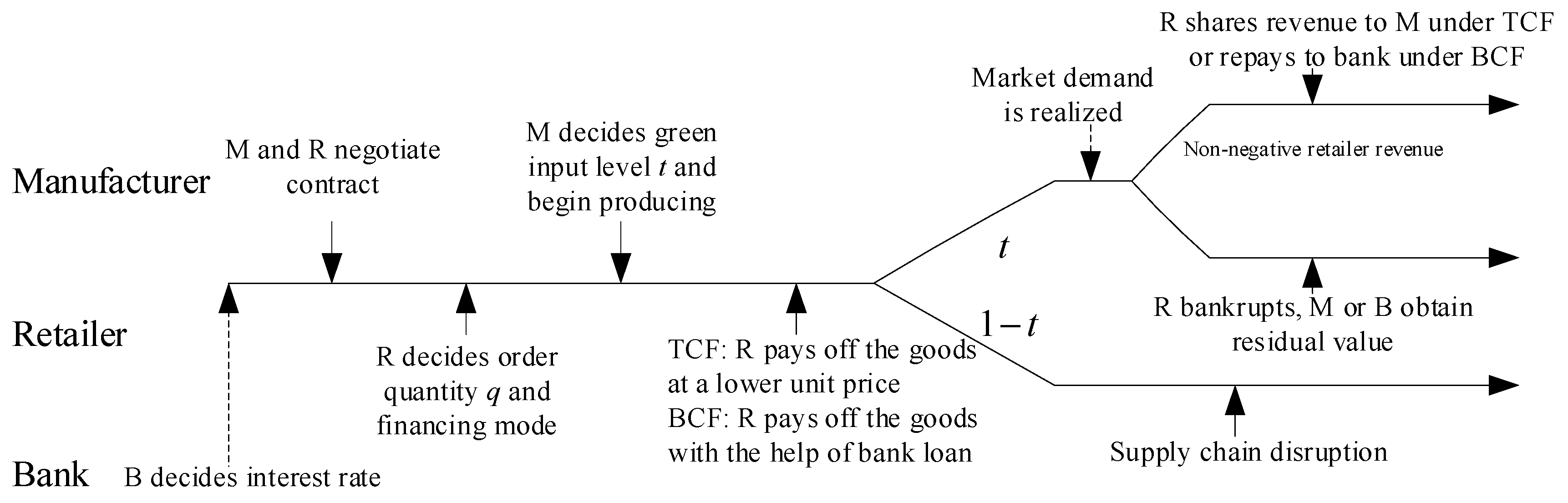
Figure 2.
Different values of .
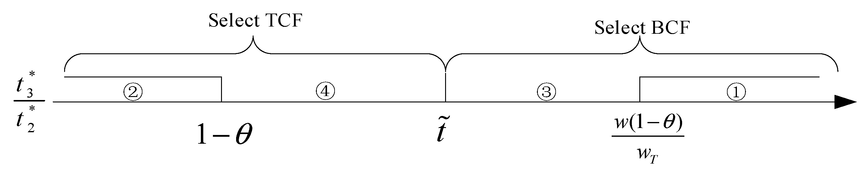
Figure 3.
The relationship between and , at .

Figure 4.
Comparison of profit under different and .

Figure 5.
Changing trend of on under TCF.

Figure 6.
Comparison of profit under different and .

Figure 7.
Changing trend of on under BCF.


Table 1.
Summary of related studies and their contributions.
| Existing Studies | Findings and Contributions | Capital Constrained | Cleaner Production | Disruption Risk |
|---|---|---|---|---|
| Wu et al. [4] | Optimal operational decisions of supply chain members under the bank and trade financing mode. | √ | √ | |
| Kouvelis and Zhao [32] | Trade credit financing can diversify the supply chain when there is a risk of insolvency and cost of default. | √ | ||
| Phan et al. [47] | They studied the role of trade credit in a capital-constrained supply chain. | √ | ||
| Cao and Yu [48] | They studied the effect of capital on the selection of a centralized supply chain financing mode and willingness to cooperate. | √ | ||
| Zou et al. [37] | They studied the impact of capital on supply chain financing and operations. | √ | √ | |
| Yang et al. [27] | Remanufacturing can be an effective way to increase carbon reduction levels and profit for manufacturers and retailers. | √ | ||
| Liu et al. [26] | The relationship between investment in carbon reduction on market demand and profitability in the agricultural supply chain. | √ | ||
| Fang and Xu [7] | The impact of carbon emission policies on green supply chain emission reduction. | √ | ||
| Yavari and Zaker [49] | The design of a resilient, green, closed-loop supply chain network for perishable products at the risk of power network disruption. | √ | ||
| Li et al. [41] | The paper examined a retailer’s multi-channel sourcing and pricing strategy under supply disruption risk. | √ | ||
| Our paper | The retailer’s financing preference and willingness to order depend on the input level of cleaner production. | √ | √ | √ |
Table 2.
Notations.
| Symbols | Definition |
|---|---|
| Manufacturer’s unit production cost | |
| Retailer’s order quantity (decision variable) | |
| Optimal order quantity (decision variable) | |
| Unit wholesale price under BCF, with | |
| Unit wholesale price under TCF, with | |
| Retail price, with | |
| Initial capital of the retailer | |
| Stochastic market demand | |
| Manufacturer’s excepted profit (decision variable) | |
| Retailer’s excepted profit (decision variable) | |
| Revenue sharing ratio, with | |
| Input level of cleaner production, with , (decision variable) | |
| The lowest input level of cleaner production, with | |
| The loan interest rate of bank, with |
Table 3.
Order decisions and profit of no-financing mode.
| 7.50 | 23.44 | 1.88 | 4.92 |
| 10.35 | 32.34 | 2.59 | 7.76 |
| 13.20 | 41.25 | 3.30 | 10.60 |
| 16.05 | 50.16 | 4.01 | 13.44 |
| 18.90 | 59.06 | 4.73 | 16.28 |
| 21.75 | 67.97 | 5.44 | 19.12 |
| 24.60 | 76.88 | 6.15 | 21.96 |
| 27.45 | 85.78 | 6.86 | 24.80 |
| 30.30 | 94.69 | 7.58 | 27.65 |
| 33.15 | 103.59 | 8.29 | 30.49 |
| 36.00 | 112.50 | 9.00 | 33.33 |
Table 4.
Computational results under TCF with different and .
| 0.013 | 7.50 | 23.44 | 333.38 | 4.33 | 0.41 | 1.88 | 30.82 | 4.92 | 5.28 | 2.46 |
| 0.016 | 7.92 | 24.73 | 316.59 | 5.08 | 0.42 | 1.98 | 31.43 | 5.33 | 5.95 | 2.36 |
| 0.020 | 8.45 | 26.41 | 299.81 | 6.00 | 0.45 | 2.11 | 32.12 | 5.86 | 6.75 | 2.24 |
| 0.040 | 11.21 | 35.02 | 248.98 | 10.03 | 0.54 | 2.80 | 34.53 | 8.61 | 10.07 | 1.85 |
| 0.061 | 13.96 | 43.63 | 221.23 | 13.41 | 0.62 | 3.49 | 35.90 | 11.36 | 12.61 | 1.62 |
| 0.081 | 16.72 | 52.23 | 202.32 | 16.37 | 0.68 | 4.18 | 36.72 | 14.10 | 14.67 | 1.47 |
| 0.101 | 19.47 | 60.84 | 188.04 | 19.03 | 0.74 | 4.87 | 37.20 | 16.85 | 16.39 | 1.35 |
| 0.122 | 22.23 | 69.45 | 176.61 | 21.46 | 0.79 | 5.56 | 37.44 | 19.60 | 17.85 | 1.26 |
| 0.142 | 24.98 | 78.06 | 167.09 | 23.69 | 0.84 | 6.25 | 37.52 | 22.34 | 19.10 | 1.19 |
| 0.162 | 27.74 | 86.67 | 158.95 | 25.77 | 0.88 | 6.93 | 37.47 | 25.09 | 20.16 | 1.13 |
| 0.182 | 30.49 | 95.28 | 151.84 | 27.70 | 0.93 | 7.62 | 37.33 | 27.83 | 21.07 | 1.08 |
| 0.203 | 33.25 | 103.89 | 145.55 | 29.50 | 0.97 | 8.31 | 37.11 | 30.58 | 21.85 | 1.03 |
| 0.223 | 36.00 | 112.50 | 139.89 | 31.20 | 1.00 | 9.00 | 36.84 | 33.33 | 22.50 | 0.99 |
Table 5.
Computational results under BCF with different and .
| 0.143 | 7.50 | 52.45 | 153.87 | 22.00 | 0.67 | 13.48 | 30.31 | 4.89 | 14.75 | 1.64 |
| 0.163 | 10.61 | 65.22 | 147.48 | 23.98 | 0.71 | 15.48 | 30.82 | 7.98 | 15.75 | 1.75 |
| 0.185 | 14.15 | 76.49 | 141.07 | 26.10 | 0.76 | 16.44 | 31.23 | 11.51 | 16.76 | 1.87 |
| 0.203 | 17.00 | 83.74 | 136.45 | 27.70 | 0.79 | 16.50 | 31.45 | 14.36 | 17.46 | 1.96 |
| 0.221 | 19.85 | 89.82 | 132.22 | 29.22 | 0.83 | 16.08 | 31.59 | 17.20 | 18.09 | 2.05 |
| 0.239 | 22.70 | 94.98 | 128.33 | 30.67 | 0.86 | 15.29 | 31.67 | 20.05 | 18.64 | 2.13 |
| 0.257 | 25.55 | 99.42 | 124.71 | 32.05 | 0.89 | 14.22 | 31.69 | 22.89 | 19.13 | 2.21 |
| 0.275 | 28.40 | 103.27 | 121.34 | 33.37 | 0.93 | 12.91 | 31.67 | 25.74 | 19.55 | 2.28 |
| 0.293 | 31.25 | 106.66 | 118.18 | 34.63 | 0.96 | 11.41 | 31.60 | 28.58 | 19.91 | 2.36 |
| 0.311 | 34.10 | 109.65 | 115.21 | 35.83 | 0.98 | 9.76 | 31.50 | 31.43 | 20.21 | 2.43 |
| 0.323 | 36.00 | 111.46 | 113.32 | 36.60 | 1.00 | 8.58 | 31.41 | 33.33 | 20.39 | 2.48 |
Disclaimer/Publisher’s Note: The statements, opinions and data contained in all publications are solely those of the individual author(s) and contributor(s) and not of MDPI and/or the editor(s). MDPI and/or the editor(s) disclaim responsibility for any injury to people or property resulting from any ideas, methods, instructions or products referred to in the content. |
© 2023 by the authors. Licensee MDPI, Basel, Switzerland. This article is an open access article distributed under the terms and conditions of the Creative Commons Attribution (CC BY) license (https://creativecommons.org/licenses/by/4.0/).
Share and Cite
MDPI and ACS Style
Cheng, J.; Hong, W.; Cheng, J. Optimal Green Input Level for a Capital-Constrained Supply Chain Considering Disruption Risk. Sustainability 2023, 15, 12095. https://doi.org/10.3390/su151512095
AMA Style
Cheng J, Hong W, Cheng J. Optimal Green Input Level for a Capital-Constrained Supply Chain Considering Disruption Risk. Sustainability. 2023; 15(15):12095. https://doi.org/10.3390/su151512095
Chicago/Turabian StyleCheng, Junheng, Weiyi Hong, and Jingya Cheng. 2023. "Optimal Green Input Level for a Capital-Constrained Supply Chain Considering Disruption Risk" Sustainability 15, no. 15: 12095. https://doi.org/10.3390/su151512095
Note that from the first issue of 2016, this journal uses article numbers instead of page numbers. See further details here.