
Optimizing Vehicle Replacement in Sustainable Urban Freight Transportation Subject to Presence of Regulatory Measures


Abstract
:1. Introduction
2. Fleet Replacement Problem
3. Materials and Methods
3.1. Problem Setting
3.2. Formulation of the Problem
- : number of vehicles of type k and age i used in zone z during year t;
- : number of salvaged vehicles of type k and age i at the end of year t;
- : number of vehicles of type k purchased at the beginning of year t.
3.3. Elasticity Analysis
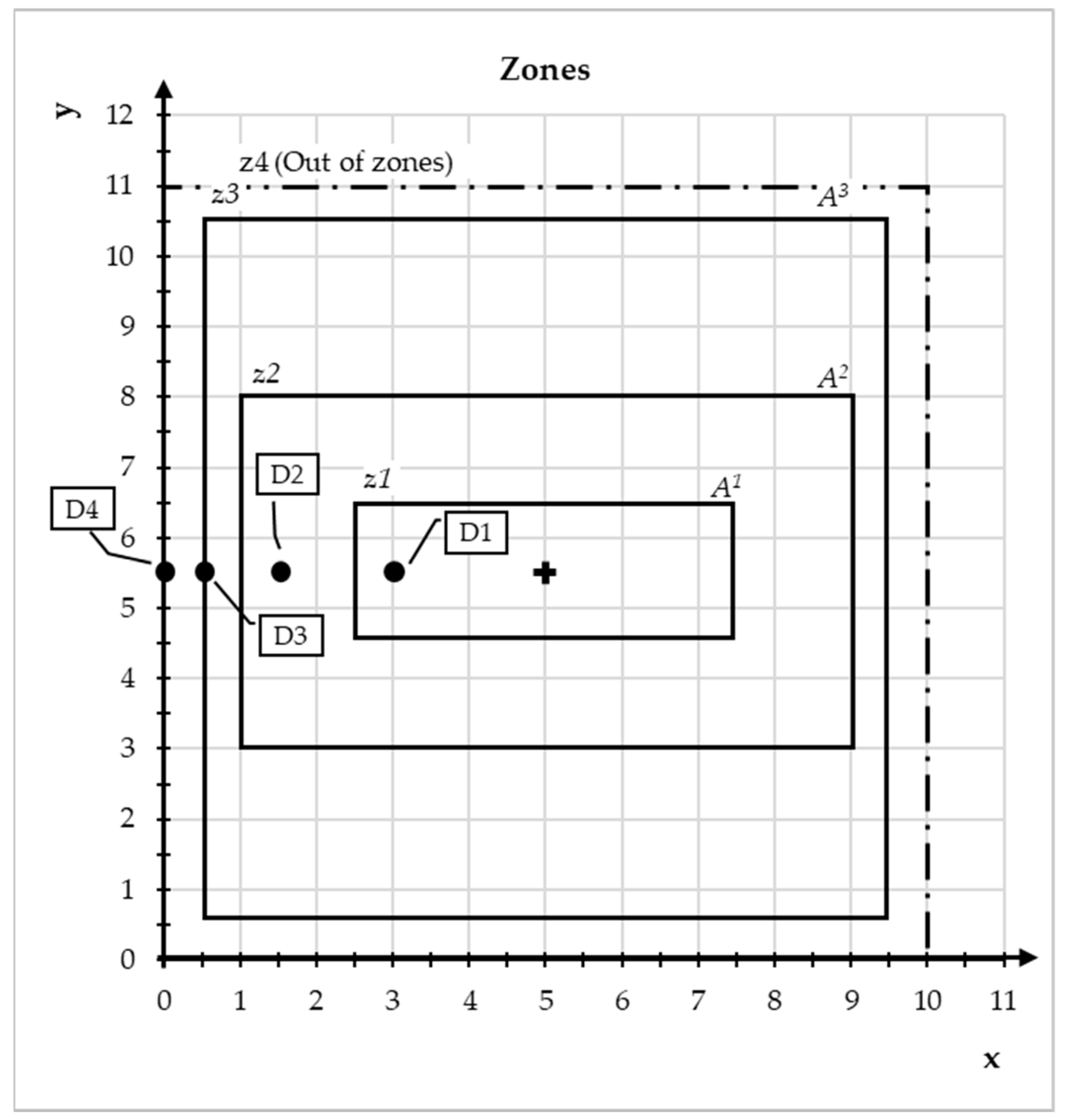
3.4. Zone Characterization
- S1: each zone has its own depot points (D1, D2 and D3);
- S2: depot points are located only in zone 2 and zone 3 (D2 and D3);
- S3: depot point is located only in zone 3 (D3);
- S4: depot point is out of all zones and in the suburb of the city (D4);
- S5: all vehicle types can access all zones, each with its own depot points (D1, D2, and D3).
3.5. Vehicle Characterization
3.6. Demand and Fleet Composition
- Light-size vehicles can serve c1 = 6 customers;
- Medium-size vehicles can serve c2 = 12 customers;
- Heavy vehicles can serve c3 = 36 customers.
4. Results and Discussion
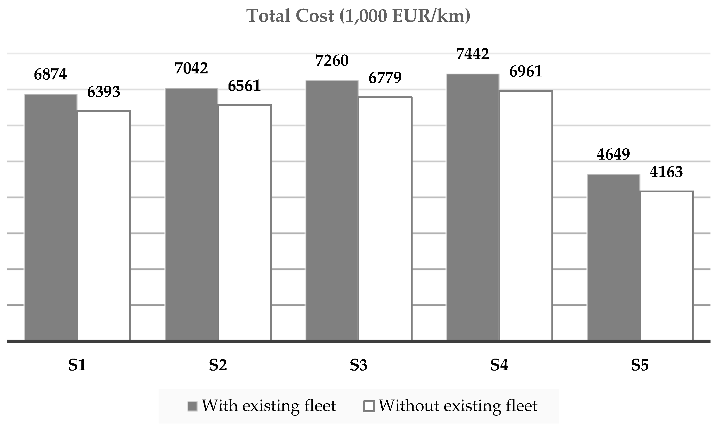
4.1. Total Cost
4.2. Fleet Composition
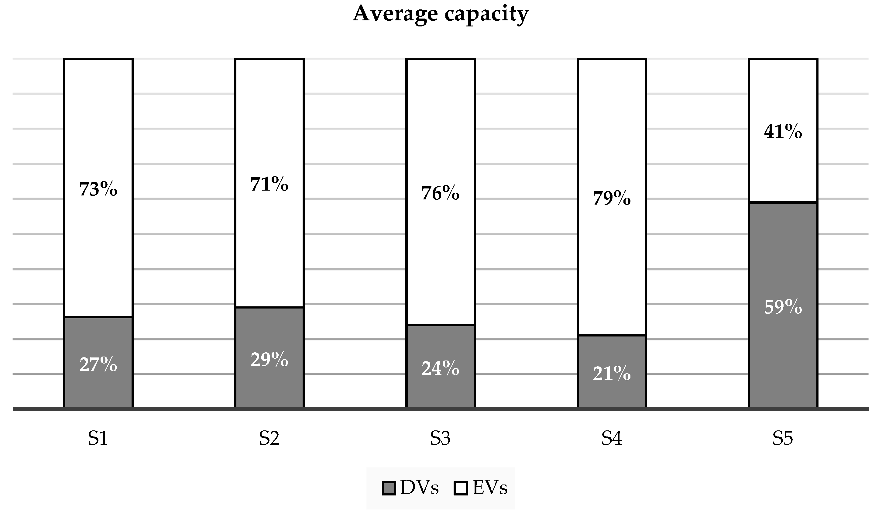
4.3. Capacity Analysis
4.4. Elasticity Analysis
4.5. Limitations and Future Research
5. Conclusions
Author Contributions
Funding
Institutional Review Board Statement
Informed Consent Statement
Data Availability Statement
Conflicts of Interest
References
- European Commission Urbanisation Worldwide. Available online: https://knowledge4policy.ec.europa.eu/foresight/topic/continuing-urbanisation/urbanisation-worldwide_en (accessed on 9 June 2020).
- Sheth, M.; Butrina, P.; Goodchild, A.; McCormack, E. Measuring Delivery Route Cost Trade-offs between Electric-Assist Cargo Bicycles and Delivery Trucks in Dense Urban Areas. Eur. Transp. Res. Rev. 2019, 11, 12. [Google Scholar] [CrossRef] [Green Version]
- Bosona, T. Urban Freight Last Mile Logistics—Challenges and Opportunities to Improve Sustainability: A Literature Review. Sustainability 2020, 12, 8769. [Google Scholar] [CrossRef]
- Cardenas, I.; Borbon-Galvez, Y.; Verlinden, T.; Van De Voorde, E.; Vanelslander, T.; Dewulf, W. City Logistics, Urban Goods Distribution and Last Mile Delivery and Collection. Compet. Regul. Netw. Ind. 2017, 18, 22–43. [Google Scholar] [CrossRef]
- Melacini, M.; Perotti, S.; Rasini, M.; Tappia, E. E-Fulfilment and Distribution in Omni-Channel Retailing: A Systematic Literature Review. Int. J. Phys. Distrib. Logist. Manag. 2018, 48, 391–414. [Google Scholar] [CrossRef]
- Macharis, C.; Kin, B. The 4 A’s of Sustainable City Distribution: Innovative Solutions and Challenges Ahead. Int. J. Sustain. Transp. 2017, 11, 59–71. [Google Scholar] [CrossRef]
- Letnik, T.; Hanžič, K.; Luppino, G.; Mencinger, M. Impact of Logistics Trends on Freight Transport Development in Urban Areas. Sustainability 2022, 14, 16551. [Google Scholar] [CrossRef]
- Riccardi, M.R.; Mauriello, F.; Sarkar, S.; Galante, F.; Scarano, A.; Montella, A. Parametric and Non-Parametric Analyses for Pedestrian Crash Severity Prediction in Great Britain. Sustainability 2022, 14, 3188. [Google Scholar] [CrossRef]
- Montella, A.; Marzano, V.; Mauriello, F.; Vitillo, R.; Fasanelli, R.; Pernetti, M.; Galante, F. Development of Macro-Level Safety Performance Functions in the City of Naples. Sustainability 2019, 11, 1871. [Google Scholar] [CrossRef] [Green Version]
- Ville, S.; Gonzalez-Feliu, J.; Dablanc, L. The Limits of Public Policy Intervention in Urban Logistics: Lessons from Vicenza (Italy). Eur. Plan. Stud. 2013, 21, 1528–1541. [Google Scholar] [CrossRef]
- Lindholm, M. Urban Freight Transport from a Local Authority Perspective-A Literature Review. Eur. Transp.-Trasp. Eur. 2013, 54, 1–37. [Google Scholar]
- Nuzzolo, A.; Comi, A. Urban Freight Transport Policies in Rome: Lessons Learned and the Road Ahead. J. Urban. 2015, 8, 133–147. [Google Scholar] [CrossRef] [Green Version]
- Maxner, T.; Chiara, G.D.; Goodchild, A. Identifying the Challenges to Sustainable Urban Last-Mile Deliveries: Perspectives from Public and Private Stakeholders. Sustainability 2022, 14, 4701. [Google Scholar] [CrossRef]
- Masłowski, D.; Kulińska, E.; Komada, G. Impact of Alternative Forms of Transport on Urban Freight Congestion. Sustainability 2022, 14, 10972. [Google Scholar] [CrossRef]
- Browne, M.; Allen, J. Enhancing the Sustainability of Urban Freight Transport and Logistics. Transp. Commun. Bull. Asia Pacific 2011, 44, 1–19. [Google Scholar]
- Comi, A.; Site, P.D.; Filippi, F.; Marcucci, E.; Nuzzolo, A. Differentiated Regulation of Urban Freight Traffic: Conceptual Framework and Examples from Italy. In Proceedings of the 13th International Conference of Hong Kong Society for Transportation Studies: Transportation and Management, Hong Kong, China, 13–15 December 2008; pp. 815–824. [Google Scholar]
- Barter, G.E.; Reichmuth, D.; Westbrook, J.; Malczynski, L.A.; West, T.H.; Manley, D.K.; Guzman, K.D.; Edwards, D.M. Parametric Analysis of Technology and Policy Tradeoffs for Conventional and Electric Light-Duty Vehicles. Energy Policy 2012, 46, 473–488. [Google Scholar] [CrossRef]
- Lebeau, P.; Macharis, C.; Van Mierlo, J.; Lebeau, K. Electrifying Light Commercial Vehicles for City Logistics? A Total Cost of Ownership Analysis. Eur. J. Transp. Infrastruct. Res. 2015, 15, 551–569. [Google Scholar] [CrossRef]
- Crist, P. Elecric Vehicles Revisited-Costs, Subsidies and Prospects; OECD Publishing: Paris, France, 2012. [Google Scholar]
- Tipagornwong, C.; Figliozzi, M. Analysis of Competitiveness of Freight Tricycle Delivery Services in Urban Areas. Transp. Res. Rec. 2014, 2410, 76–84. [Google Scholar] [CrossRef] [Green Version]
- Feng, W.; Figliozzi, M. An Economic and Technological Analysis of the Key Factors Affecting the Competitiveness of Electric Commercial Vehicles: A Case Study from the USA Market. Transp. Res. Part C Emerg. Technol. 2013, 26, 135–145. [Google Scholar] [CrossRef]
- Taefi, T.T.; Kreutzfeldt, J.; Held, T.; Konings, R.; Kotter, R.; Lilley, S.; Baster, H.; Green, N.; Laugesen, M.S.; Jacobsson, S.; et al. Comparative Analysis of European Examples of Freight Electric Vehicles Schemes—A Systematic Case Study Approach with Examples from Denmark, Germany, the Netherlands, Sweden and the UK. In Dynamics in Logistics-Proceedings of the 4th International Conference LDIC, 2014, Bremen, Germany, 10–14 February 2014; Kotzab, H., Pannek, J., Thoben, K.D., Eds.; Springer International Publishing: Cham, Switzerland, 2016; pp. 495–504. ISBN 9783319235127. [Google Scholar]
- Kokate, V.; Holmukhe, R.M.; Karandikar, P.B.; Bankar, D.S.; Aparaj, P. Optimization of Battery-Ultracapacitor for Electrically Operated Vehicle for Urban Driving Cycle in India. Int. J. Sci. Technol. Res. 2020, 9, 7270–7274. [Google Scholar]
- Dablanc, L. Goods Transport in Large European Cities: Difficult to Organize, Difficult to Modernize. Transp. Res. Part A Policy Pract. 2007, 41, 280–285. [Google Scholar] [CrossRef]
- Behiri, W.; Belmokhtar-Berraf, S.; Chu, C. Urban Freight Transport Using Passenger Rail Network: Scientific Issues and Quantitative Analysis. Transp. Res. Part E Logist. Transp. Rev. 2018, 115, 227–245. [Google Scholar] [CrossRef]
- Nina, M. Introduction of Electric Vehicles in Portugal-A Cost-Benefit Analysis; Instituto Superior Técnico, Universidade de Lisboa: Lisboa, Portugal, 2010. [Google Scholar]
- Scarf, P.A.; Bouamra, O. Capital Equipment Replacement Model for a Fleet with Variable Size. J. Qual. Maint. Eng. 1999, 5, 40–49. [Google Scholar] [CrossRef]
- Redmer, A. Optimisation of the Exploitation Period of Individual Vehicles in Freight Transportation Companies. Transp. Res. Part E Logist. Transp. Rev. 2009, 45, 978–987. [Google Scholar] [CrossRef]
- Rees, L.P.; Clayton, E.R.; Taylor, B.W. A Network Simulation Model for Police Patrol Vehicle Maintenance and Replacement Analysis. Comput. Environ. Urban Syst. 1982, 7, 191–196. [Google Scholar] [CrossRef]
- Suzuki, Y.; Pautsch, G.R. A Vehicle Replacement Policy for Motor Carriers in an Unsteady Economy. Transp. Res. Part A Policy Pract. 2005, 39, 463–480. [Google Scholar] [CrossRef]
- Kim, H.C.; Keoleian, G.A.; Grande, D.E.; Bean, J.C. Life Cycle Optimization of Automobile Replacement: Model and Application. Environ. Sci. Technol. 2003, 37, 5407–5413. [Google Scholar] [CrossRef]
- Emiliano, W.; Alvelos, F.; Telhada, J.; Lanzer, E.A. An Optimization Model for Bus Fleet Replacement with Budgetary and Environmental Constraints. Transp. Plan. Technol. 2020, 43, 488–502. [Google Scholar] [CrossRef]
- Akogbe, R.-K.T.M.; Feng, X.; Zhou, J. Importance and Ranking Evaluation of Delay Factors for Development Construction Projects in Benin. KSCE J. Civ. Eng. 2013, 17, 1213–1222. [Google Scholar] [CrossRef]
- Li, L.; Lo, H.K.; Xiao, F.; Cen, X. Mixed Bus Fleet Management Strategy for Minimizing Overall and Emissions External Costs. Transp. Res. Part D Transp. Environ. 2018, 60, 104–118. [Google Scholar] [CrossRef]
- Redmer, A. Strategic Vehicle Fleet Management–a Joint Solution of Make-or-Buy, Composition and Replacement Problems. J. Qual. Maint. Eng. 2022, 28, 327–349. [Google Scholar] [CrossRef]
- Zheng, S.; Chen, S. Fleet Replacement Decisions under Demand and Fuel Price Uncertainties. Transp. Res. Part D Transp. Environ. 2018, 60, 153–173. [Google Scholar] [CrossRef]
- Raposo, H.; Farinha, J.T.; Ferreira, L.; Galar, D. An Integrated Econometric Model for Bus Replacement and Determination of Reserve Fleet Size Based on Predictive Maintenance. Eksploat. I Niezawodn. 2017, 19, 358–368. [Google Scholar] [CrossRef]
- Koç, Ç.; Bektaş, T.; Jabali, O.; Laporte, G. The Impact of Depot Location, Fleet Composition and Routing on Emissions in City Logistics. Transp. Res. Part B Methodol. 2016, 84, 81–102. [Google Scholar] [CrossRef]
- Daganzo, C.F. Modeling Distribution Problems with Time Windows: Part I. Transp. Sci. 1987, 21, 171–179. [Google Scholar] [CrossRef]
- Allen, R.G.D. The Concept of Arc Elasticity of Demand: I. Rev. Econ. Stud. 1934, 1, 226–229. [Google Scholar] [CrossRef]
- Ahani, P.; Arantes, A.; Melo, S. A Portfolio Approach for Optimal Fleet Replacement toward Sustainable Urban Freight Transportation. Transp. Res. Part D Transp. Environ. 2016, 48, 357–368. [Google Scholar] [CrossRef]
- Ghiani, G.; Laporte, G.; Musmanno, R. Introduction to Logistics Systems Management, 3rd ed.; John Wiley and Sons Ltd.: Hoboken, NJ, USA, 2022; ISBN 9781119789390. [Google Scholar]
- Meusalario.pt Compare Seu Salário. Available online: https://meusalario.pt/salario/compare-seu-salario?job-id=8322020000000/%5C#/ (accessed on 6 July 2020).
- NISSAN NISSAN E-NV200. Available online: https://www.nissan.pt/veiculos/novos-veiculos/e-nv200/preco-e-versoes.html (accessed on 6 May 2020).
- ACEA Average Age of the EU Vehicle Fleet, by Country. Available online: https://www.acea.auto/figure/average-age-of-eu-vehicle-fleet-by-country/ (accessed on 22 July 2020).
- PORDATA Consumo de Energia Elétrica: Total e Por Setor de Atividade Económica. Available online: https://www.pordata.pt/Portugal (accessed on 22 July 2020).
- Zhang, J.; Wang, Z.; Liu, P.; Cui, D.; Li, X. Analysis on Influence Factors of Energy Consumption of Electric Vehicles Based on Real-World Driving Data. In Proceedings of the International Conference on Applied Energy 2019, Västerås, Sweden, 12–15 August 2019; pp. 12–15. [Google Scholar]
- Lois, D.; Wang, Y.; Boggio-Marzet, A.; Monzon, A. Multivariate Analysis of Fuel Consumption Related to Eco-Driving: Interaction of Driving Patterns and External Factors. Transp. Res. Part D Transp. Environ. 2019, 72, 232–242. [Google Scholar] [CrossRef]
- Adeniran, I.O. The Impacts of Sustainable Concepts in Urban Freight Distribution—A Courier, Express and Parcel Case Study; TUM-Technische Universität München: Munich, Germany, 2020. [Google Scholar]
- Feng, R.; Hu, X.; Li, G.; Sun, Z.; Ye, M.; Deng, B. Exploration on the Emissions and Catalytic Reactors Interactions of a Non-Road Diesel Engine through Experiment and System Level Simulation. Fuel 2023, 342, 127746. [Google Scholar] [CrossRef]
- Gerlagh, R.; Heijmans, R.J.R.K.; Rosendahl, K.E. COVID-19 Tests the Market Stability Reserve. Environ. Resour. Econ. 2020, 76, 855–865. [Google Scholar] [CrossRef]
- Lee, D.Y.; Thomas, V.M.; Brown, M.A. Electric Urban Delivery Trucks: Energy Use, Greenhouse Gas Emissions, and Cost-Effectiveness. Environ. Sci. Technol. 2013, 47, 8022–8030. [Google Scholar] [CrossRef]
- City of Toronto-Fleet Services 2017 Performance Measurement & Benchmarking Report. Available online: https://www.toronto.ca/wp-content/uploads/2019/05/8f5d-FleetServices2017-PMBR-Finalv2-AODA.pdf (accessed on 15 April 2023).
- Electrification Coalition Fleet Electrification Roadmap: Revolutionizing Transportation and Achieving Energy Security. Available online: https://www.electrificationcoalition.org/wp-content/uploads/2018/07/EC-Fleet-Roadmap-screen.pdf (accessed on 15 April 2023).
- Pettersson, A.I.; Segerstedt, A. Measuring Supply Chain Cost. Int. J. Prod. Econ. 2013, 143, 357–363. [Google Scholar] [CrossRef]


| Zone | Coordinates (x, y) of the Left-Down Corner of Each Zone (km, km) | Outer Dimensions of Each Zone (km × km) | (km2) | Coordinates (x, y) of Each Depot (km, km) | |
|---|---|---|---|---|---|
| z1 | 2.5, 4.5 | 5 × 2 | 10 | 3.0, 5.5 | 2.0 |
| z2 | 1.0, 3.0 | 8 × 5 | 30 | 1.5, 5.5 | 3.5 |
| z3 | 0.5, 0.5 | 9 × 10 | 50 | 0.5, 5.5 | 4.5 |
| Suburban zone (Out of zones) | 0.0, 0.0 | 10 × 11 | 20 | 0.0, 5.5 | 5.0 |
| k | Vehicle Model | Motor Type | Size Type | Capacity (m3) | Price (Euro) | Driver Salary (EUR/Month) [43] | Energy Consumption |
|---|---|---|---|---|---|---|---|
| 1 | Renault New Kangoo Express [18] | Diesel | Light | 2 | 13,600 | 750 | 5.2 l/100 km |
| 2 | Renault Kangoo ZE [18] | Electric | Light | 2 | 21,150 | 750 | 15.5 kWh:100 km |
| 3 | Nissan NV200 [18] | Diesel | Medium | 4 | 15,400 | 932 | 5.7 L/100 km |
| 4 | Nissan e-NV200 [44] | Electric | Medium | 4 | 25,652 | 932 | 16.5 k Wh:100 km |
| 5 | Isuzu N-Series [21] | Diesel | Heavy | 12 | 48,450 | 1068 | 17.47 L/100 km |
| 6 | eStar (Navistar) [21] | Electric | Heavy | 12 | 133,369 | 1068 | 50 kWh:100 km |
| Parameter | Diesel Vehicle | Electric Vehicle |
|---|---|---|
| Maximum age (Ak) [21,45] | 15 | |
| Discount rate(dr) [21] | 6.50% | |
| Working days in a year (Wd) | 251 | |
| Planning time horizon(year) (t) [21] | 30 | |
| Depreciation rate (θk) [21,41] | 0.15 | 0.198 |
| Energy cost growth rate (fd, fe) [46] | 0.0582 | 0.0289 |
| Energy consumption (Rk, Qk) [47,48] | 0.062 L/km | 0.145 kWh/km |
| Energy cost [46] | 1.167 EUR/L | 0.167 EUR/kWh |
| CO2 emissions (Well-to-Wheel) [49,50] | 2.63 kg/L | 0.47 kg/kWh |
| Zone | Demand (Customer/Day) | LDV | MDV | HDV |
|---|---|---|---|---|
| z1 | n1 = 60 | 10 | - | - |
| z2 | n2 = 90 | 5 | 5 | - |
| z3 | n3 = 120 | 4 | 2 | 2 |
| Total | 270 | 19 1 | 7 | 2 |
| Scenario | Vehicle Type | Average Usage | Initial Usage | Final Usage | ||||||
|---|---|---|---|---|---|---|---|---|---|---|
| z1 | z2 | z3 | z1 | z2 | z3 | z1 | z2 | z3 | ||
| S1 | LDV | 0.033 | 0 | 0 | 1 | 0 | 0 | 0 | 0 | 0 |
| LEV | 9.967 | 0 | 0 | 9 | 0 | 0 | 10 | 0 | 0 | |
| MDV | 0 | 2.133 | 0 | 0 | 8 | 0 | 0 | 0 | 0 | |
| MEV | 0 | 5.867 | 0 | 0 | 0 | 0 | 0 | 8 | 0 | |
| HDV | 0 | 0 | 1.067 | 0 | 0 | 4 | 0 | 0 | 0 | |
| HEV | 0 | 0 | 2.933 | 0 | 0 | 0 | 0 | 0 | 4 | |
| S2 | LDV | 1.267 | 0 | 0 | 10 | 0 | 0 | 0 | 0 | 0 |
| LEV | 8.733 | 0 | 0 | 0 | 0 | 0 | 10 | 0 | 0 | |
| MDV | 0 | 2.133 | 0 | 0 | 8 | 0 | 0 | 0 | 0 | |
| MEV | 0 | 5.867 | 0 | 0 | 0 | 0 | 0 | 8 | 0 | |
| HDV | 0 | 0 | 1.067 | 0 | 0 | 4 | 0 | 0 | 0 | |
| HEV | 0 | 0 | 2.933 | 0 | 0 | 0 | 0 | 0 | 4 | |
| S3 | LDV | 0.7 | 0 | 0 | 10 | 0 | 0 | 0 | 0 | 0 |
| LEV | 9.3 | 0 | 0 | 0 | 0 | 0 | 10 | 0 | 0 | |
| MDV | 0 | 1.6 | 0 | 0 | 8 | 0 | 0 | 0 | 0 | |
| MEV | 0 | 6.4 | 0 | 0 | 0 | 0 | 0 | 8 | 0 | |
| HDV | 0 | 0 | 1.067 | 0 | 0 | 4 | 0 | 0 | 0 | |
| HEV | 0 | 0 | 2.933 | 0 | 0 | 0 | 0 | 0 | 4 | |
| S4 | LDV | 0.933 | 0 | 0 | 10 | 0 | 0 | 0 | 0 | 0 |
| LEV | 9.067 | 0 | 0 | 0 | 0 | 0 | 10 | 0 | 0 | |
| MDV | 0 | 1.067 | 0 | 0 | 8 | 0 | 0 | 0 | 0 | |
| MEV | 0 | 6.933 | 0 | 0 | 0 | 0 | 0 | 8 | 0 | |
| HDV | 0 | 0 | 1.3 | 0 | 0 | 4 | 0 | 0 | 0 | |
| HEV | 0 | 0 | 2.7 | 0 | 0 | 0 | 0 | 0 | 4 | |
| S5 | LDV | 0 | 0.033 | 0 | 0 | 1 | 0 | 0 | 0 | 0 |
| LEV | 0 | 0 | 0 | 0 | 0 | 0 | 0 | 0 | 0 | |
| MDV | 0 | 0.4 | 0.167 | 0 | 1 | 1 | 0 | 0 | 0 | |
| MEV | 0.467 | 1.567 | 0.667 | 0 | 0 | 0 | 2 | 2 | 1 | |
| HDV | 1.6 | 1.567 | 2.233 | 2 | 2 | 3 | 0 | 0 | 0 | |
| HEV | 0.167 | 0.433 | 0.933 | 0 | 0 | 0 | 1 | 2 | 3 | |
| Scenario | Vehicle Type | Average Usage | Initial Usage | Final Usage | ||||||
|---|---|---|---|---|---|---|---|---|---|---|
| z1 | z2 | z3 | z1 | z2 | z3 | z1 | z2 | z3 | ||
| S1 | LDV | 0.133 | 0 | 0 | 4 | 0 | 0 | 0 | 0 | 0 |
| LEV | 9.867 | 0 | 0 | 6 | 0 | 0 | 10 | 0 | 0 | |
| MDV | 0 | 2.133 | 0 | 0 | 8 | 0 | 0 | 0 | 0 | |
| MEV | 0 | 5.867 | 0 | 0 | 0 | 0 | 0 | 8 | 0 | |
| HDV | 0 | 0 | 1.067 | 0 | 0 | 4 | 0 | 0 | 0 | |
| HEV | 0 | 0 | 2.933 | 0 | 0 | 0 | 0 | 0 | 4 | |
| S2 | LDV | 1.267 | 0 | 0 | 10 | 0 | 0 | 0 | 0 | 0 |
| LEV | 8.733 | 0 | 0 | 0 | 0 | 0 | 10 | 0 | 0 | |
| MDV | 0 | 2.133 | 0 | 0 | 8 | 0 | 0 | 0 | 0 | |
| MEV | 0 | 5.867 | 0 | 0 | 0 | 0 | 0 | 8 | 0 | |
| HDV | 0 | 0 | 1.067 | 0 | 0 | 4 | 0 | 0 | 0 | |
| HEV | 0 | 0 | 2.933 | 0 | 0 | 0 | 0 | 0 | 4 | |
| S3 | LDV | 0.7 | 0 | 0 | 10 | 0 | 0 | 0 | 0 | 0 |
| LEV | 9.3 | 0 | 0 | 0 | 0 | 0 | 10 | 0 | 0 | |
| MDV | 0 | 1.6 | 0 | 0 | 8 | 0 | 0 | 0 | 0 | |
| MEV | 0 | 6.4 | 0 | 0 | 0 | 0 | 0 | 8 | 0 | |
| HDV | 0 | 0 | 1.067 | 0 | 0 | 4 | 0 | 0 | 0 | |
| HEV | 0 | 0 | 2.933 | 0 | 0 | 0 | 0 | 0 | 4 | |
| S4 | LDV | 0.933 | 0 | 0 | 10 | 0 | 0 | 0 | 0 | 0 |
| LEV | 9.067 | 0 | 0 | 0 | 0 | 0 | 10 | 0 | 0 | |
| MDV | 0 | 1.067 | 0 | 0 | 8 | 0 | 0 | 0 | 0 | |
| MEV | 0 | 6.933 | 0 | 0 | 0 | 0 | 0 | 8 | 0 | |
| HDV | 0 | 0 | 1.3 | 0 | 0 | 4 | 0 | 0 | 0 | |
| HEV | 0 | 0 | 2.7 | 0 | 0 | 0 | 0 | 0 | 4 | |
| S5 | LDV | 0 | 0 | 0 | 0 | 0 | 0 | 0 | 0 | 0 |
| LEV | 0 | 0 | 0 | 0 | 0 | 0 | 0 | 0 | 0 | |
| MDV | 0 | 0.433 | 0.167 | 0 | 2 | 1 | 0 | 0 | 0 | |
| MEV | 0.467 | 1.567 | 0.667 | 0 | 0 | 0 | 2 | 2 | 1 | |
| HDV | 1.6 | 1.567 | 2.333 | 2 | 2 | 3 | 0 | 0 | 0 | |
| HEV | 0.167 | 0.433 | 0.933 | 0 | 0 | 0 | 1 | 2 | 3 | |
| Parameter | Interval (%) | Baseline Value (%) | S1 | S2 | S3 | S4 | S5 | |
|---|---|---|---|---|---|---|---|---|
| With an existing fleet | EVs depreciation rate | 10 to 20 | 15 | 0.055 | 0.132 | 0.193 | 0.055 | 0.055 |
| EVs depreciation rate | 14 to 24 | 19.8 | 0.015 | 0.135 | 0.095 | 0.015 | 0.015 | |
| EVs depreciation rate | 18 to 28 | 23 | 0.025 | 0.130 | 0.048 | 0.025 | 0.025 | |
| DVs energy price growth rate | 2.91 to 8.73 | 5.82 | 0.069 | 0.005 | 0.004 | 0.069 | 0.069 | |
| EVs energy price growth rate | 1.44 to 4.33 | 2.89 | 0.016 | 0.016 | 0.026 | 0.016 | 0.016 | |
| Without an existing fleet | EVs depreciation rate | 10 to 20 | 15 | 0.091 | 0.098 | 0.118 | 0.129 | 0.055 |
| EVs depreciation rate | 14 to 24 | 19.8 | 0.052 | 0.054 | 0.079 | 0.095 | 0.015 | |
| EVs depreciation rate | 18 to 28 | 23 | 0.026 | 0.026 | 0.04 | 0.052 | 0.025 | |
| DVs energy price growth rate | 2.91 to 8.73 | 5.82 | 0.069 | 0.068 | 0.063 | 0.061 | 0.132 | |
| EVs energy price growth rate | 1.44 to 4.33 | 2.89 | 0.016 | 0.018 | 0.021 | 0.024 | 0.014 |
Disclaimer/Publisher’s Note: The statements, opinions and data contained in all publications are solely those of the individual author(s) and contributor(s) and not of MDPI and/or the editor(s). MDPI and/or the editor(s) disclaim responsibility for any injury to people or property resulting from any ideas, methods, instructions or products referred to in the content. |
© 2023 by the authors. Licensee MDPI, Basel, Switzerland. This article is an open access article distributed under the terms and conditions of the Creative Commons Attribution (CC BY) license (https://creativecommons.org/licenses/by/4.0/).
Share and Cite
Ahani, P.; Arantes, A.; Garmanjani, R.; Melo, S. Optimizing Vehicle Replacement in Sustainable Urban Freight Transportation Subject to Presence of Regulatory Measures. Sustainability 2023, 15, 12266. https://doi.org/10.3390/su151612266
Ahani P, Arantes A, Garmanjani R, Melo S. Optimizing Vehicle Replacement in Sustainable Urban Freight Transportation Subject to Presence of Regulatory Measures. Sustainability. 2023; 15(16):12266. https://doi.org/10.3390/su151612266
Chicago/Turabian StyleAhani, Parisa, Amílcar Arantes, Rohollah Garmanjani, and Sandra Melo. 2023. "Optimizing Vehicle Replacement in Sustainable Urban Freight Transportation Subject to Presence of Regulatory Measures" Sustainability 15, no. 16: 12266. https://doi.org/10.3390/su151612266
APA StyleAhani, P., Arantes, A., Garmanjani, R., & Melo, S. (2023). Optimizing Vehicle Replacement in Sustainable Urban Freight Transportation Subject to Presence of Regulatory Measures. Sustainability, 15(16), 12266. https://doi.org/10.3390/su151612266