Electric Flight in Extreme and Uncertain Urban Environments

Abstract

In a typical application scenario for electric aircraft, the emerging urban air mobility is faced with uncertain environmental conditions. To investigate the potential influence of uncertainties, this paper first develops comprehensive models of aircraft rigid body motion and electric propulsive performance. The urban environment model is built with emphasis on wind speed and the heat island effect. Thereafter, a flight guidance law augmented with nonlinear dynamic inversion is proposed to facilitate the performance evaluation of electric aircraft. Multiple simulations at various dates, times, and with different battery aging statuses are conducted. The results show that the battery aging effect and ambient temperature change are the most important factors that influence the aircraft performance. Suggestions to enhance the performance are given based on simulations.

1. Introduction

1.1. Background

With the extensive use of electric vehicles, urban transportation has continued at a steady pace towards sustainability. Given the unresolved challenges, such as traffic congestion due to the ongoing urbanization, there is an emerging consensus of opinion to further utilize urban airspace, i.e., to develop urban air mobility (UAM) [1]. The early explorations of UAM date back to the commercial helicopter flights during the 1960s, which suffer from high noise levels and non-guaranteed safety levels in complex urban environments [2]. The electric aircraft, especially those with vertical takeoff and landing (i.e., eVTOL) capability, are a potential strategy for the future sustainable UAM [3], thanks to their lower acoustic signatures, zero carbon footprint [4], and enhanced safety redundancy [5], all enabled by the novel electric propulsion system [6].

Compared to other electrified transportation platforms, such as electric ground cars and ships, the electric aircraft holds the additional advantage of exploiting the altitude change to improve the transportation efficiency [7,8,9]. This feature, in turn, results in a wider range of operational conditions [10]. Take the standard atmosphere model as an example; the ambient temperature drops by 6.5 $°\mathrm{C}$ with each increasing one-kilometer altitude [11]. If the aircraft takes off at the mean sea level and cruises at 4km [12], the external temperature drops by 26 $°\mathrm{C}$. Intuitively, the aircraft “flies across seasons” within a single mission, which distinguishes it from ground or water vehicles. Compared to those propelled by piston or turbine engines, the wide operational range of electric aircraft can lead to performance issues since they are driven by lithium-ion batteries (LIB), which are sensitive to external temperature. Moreover, the LIB as an energy supply unit, unlike fossil fuel, which is consumed in operation, is rechargeable after use. However, this characteristic also results in the aging effect. The aforementioned features, plus the polarization and diffusion effects of LIB, lead to a more complex performance of eVTOL, especially in extreme conditions.

1.2. Literature Review

It is worth noting that the term “extreme” does not refer to the worst flight conditions at arbitrary locations or altitude but is, rather, limited to the urban airspace. For instance, high-latitude regions such as Norway intend to replace their current commuter aviation networks with electrified aircraft [13]. In that case, the mean-sea-level temperature is relatively low, let alone the lower values in cruise flight. Consequently, the LIB performance dependent on the internal resistance, open-circuit voltage, and available capacity can vary in a wide range due to the so-called “thermal effect” [14]. The available performance may be insufficient, especially in winter. Analogously, for low-altitude regions such as Singapore, the ambient temperature in summer can be high, plus there is the urban heat island effect. Worse still, unlike fossil fuel, which is burned after use, the entity of the LIB is retained posterior to flight [15], making its performance deteriorate with increasing cycle numbers as a result of the aging effect [16].

All the above-mentioned unique features of the LIB, as an energy and power supply unit for UAM dependent on the temperature and aging, can be treated as uncertainties. Challenges arise from the extreme and uncertain urban environment, including, but not limited to, energy management, flight control, navigation and collision avoidance, communication and network congestion, emergency situations and failures, weather monitoring and prediction, infrastructure requirements, noise, and environmental considerations. Among others, this paper places particular attention on the long-timescale performance, such as range and energy consumption. Given the fact that eVTOL performance is still insufficient, the uncertain factors can significantly change the actual operational availability of electric aircraft. A natural concern therewith is to analyze the feasibility and availability of electric flight subject to changing ambient parameters.

An overriding requirement in such an analysis is to predict the consumed electric energy during the flight. Solely focusing on this aspect leads to a succinct modeling of the electric propulsion system by energy conversion efficiency. A rough estimation of endurance and range, as a result, is usually used in the preliminary design and policy-making. For instance, the weight trend, cost, and availability of a light electric aircraft is investigated by Rezende based on the estimation of LIB-specific energy [17]. In Ref. [18], the possibility of using several alternative sustainable energy sources in a certain area is discussed, where typical mission profiles and aircraft types are investigated based on the electric propulsive efficiency. In a similar work conducted by Trym et al. [19], the propulsion system is represented by the energy conversion efficiency of the converter, motor, gear, and propeller. The limitation and potential of electric flight in a certain area is studied on this basis. A climatology analysis by Reiche et al. [20], which takes ten metropolitan areas in the U.S. as test cases, proves that the weather conditions and public acceptance are potential barriers for future UAM scale operation.

The method of approximating the propulsion efficiency as a constant holds the advantage of low computational complexity, yet the accuracy may be insufficient, especially when considering the ever varying external conditions, which can alter the aircraft performance significantly. To reflect these complex phenomena, numerical simulations based on ordinary differential equations should be introduced. This is usually performed by augmenting the point-mass model of an aircraft with low-order electric propulsion features, such as the power conversion, energy consumption, and dynamic tuning process of thrust.

A typical example using such a modeling method can be found in Ref. [21]. The availability of electric flight in Norwegian area is explored considering environmental uncertainties (temperature, wind, and air density, to name a few). The performance (e.g., range and energy consumption) of an electric airplane subject to propulsive constraints is evaluated using aircraft trajectory optimization with high precision, which is followed by surrogate models to enable efficient uncertainty analysis. Clarke et al. [22] study a dual problem of predicting the battery lifetime regarding specific flight conditions. In specific, the mission performance of four typical aircraft types used in UAM is considered. On this basis, the aging process of LIB and its influence on aircraft performance are quantitatively studied. In the previous work conducted by the authors [14], the coupling relationship between the electric propulsion system and the airframe was extended to incorporate the thermal dynamics and battery unevenness. The influence of different ambient temperatures on the initial LIB temperature is investigated.

However, the real-world urban electric flights, especially “intracity” (i.e., inside the city, compared to “intercity”, i.e., between cities), can be more complex due to the uncertain wind and temperature conditions. This should be studied based on typical routes of UAM missions but has so far rarely or partially been addressed by the above-mentioned works. Hence, this paper focuses on developing comprehensive models for both electric aircraft and its urban operational environment, aiming to reflect the aircraft performance subject to uncertainties. The novelties of this paper are embodied in the two aspects below.

• A comprehensive simulation model is developed to reflect the influence of uncertain urban operational environments on electric aircraft performance. An urban environment model with a heat island effect and wind distribution regarding location, altitude, time, and date is developed for uncertainty quantification of UAM. The internal and external uncertain factors are considered using the ordinary differential equation, which guarantees the required modeling fidelity with relatively low complexity.
• An evaluation method is proposed to study the electric aircraft performance subject to given mission way-points. The flight guidance law is augmented with nonlinear dynamic inversion to predict the energy consumption of the electric propulsion system.

This paper is organized as below. Section 2 introduces the modeling principles of the electric aircraft with propulsive dynamics and constraints. On this basis, a novel method of flight guidance enhanced by nonlinear dynamic inversion is proposed to evaluate the aircraft performance subject to the specific mission profile. Section 3 showcases the performance of an exemplary the electric aircraft in the selected urban area subject to various uncertainties. Section 4 analyzes the simulation results. Section 5 summarizes the work and outlook of future research.

2. Materials and Methods

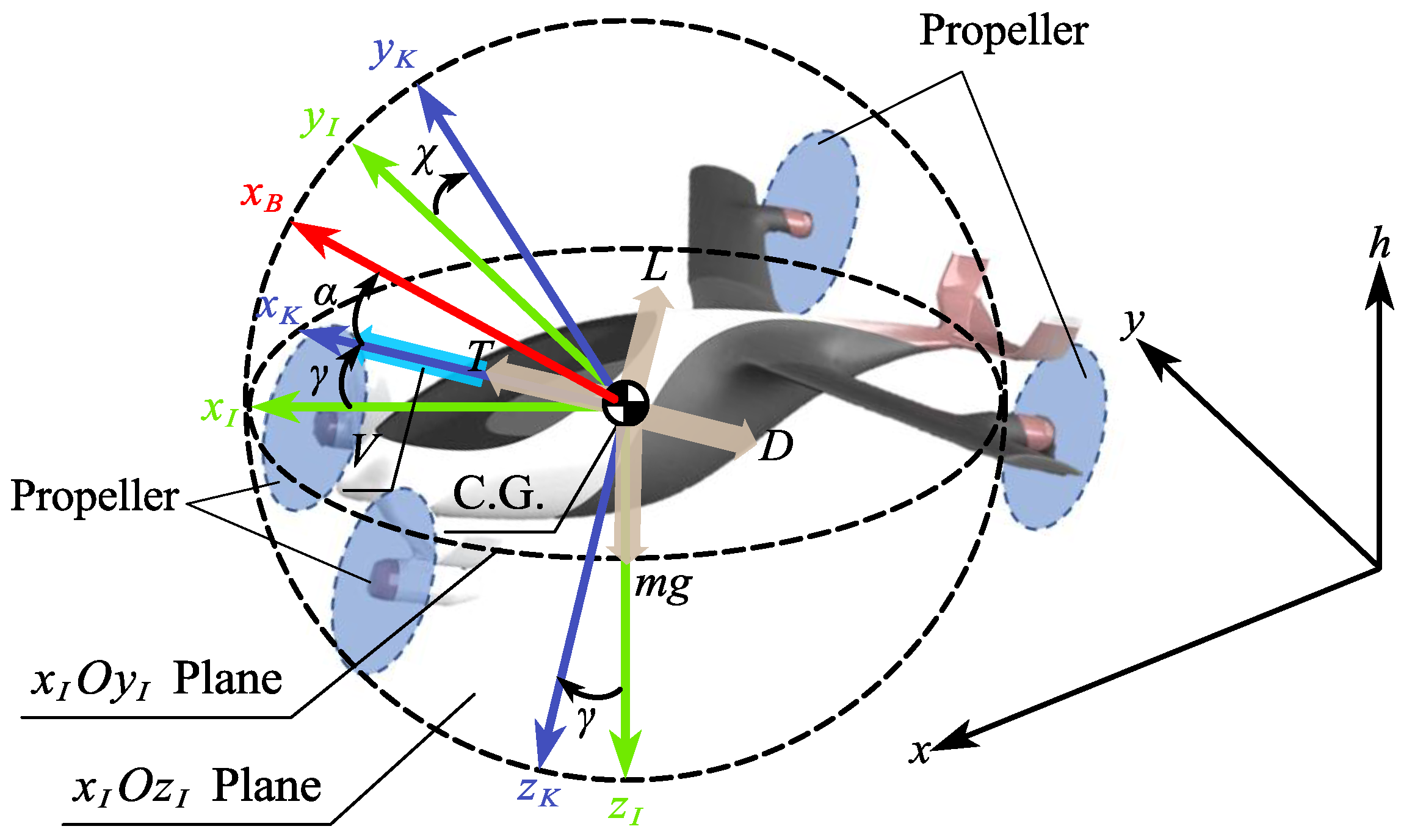
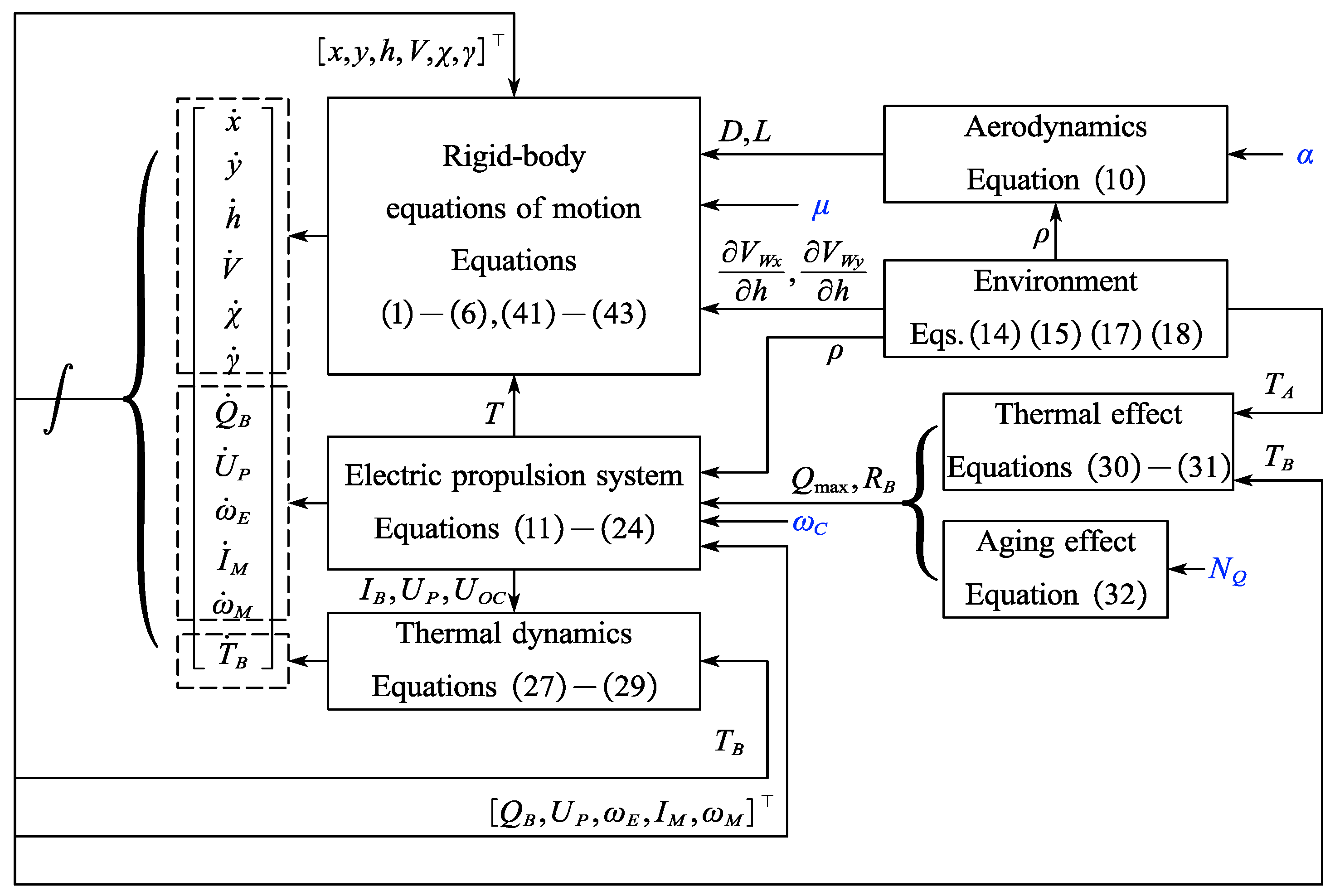
2.1. Dynamic Simulation Model of Rigid-Body Aircraft

In the UAM application scenario, it is reasonable to represent the motion of eVTOL with the three-dimensional point-mass model.

• Flat and non-rotating earth. The operational altitude is assumed to be less than 4 km [23]. The low-altitude and low-speed feature allows for this assumption;
• Rigid-body motion. Due to the limits of the UAM application scenario, the velocity of eVTOL is low compared to that of the high-speed aircraft. Hence, the aeroelasticity is omitted;
• The mass distribution is symmetric regarding the vertical plane defined in the body-frame of eVTOL;
• Time-invariant total mass. As eVTOL is driven by LIB rather than fossil fuel, there exists no mass reduction led by fuel consumption.

On this basis, we consider eVTOL aircraft with wing-borne flight capacity (e.g., tilt-rotor, tilt-wing, or hybrid configuration) since the fixed-aerodynamics are efficient for cruising. The corresponding force equilibrium and coordinates are depicted in Figure 1, where $x_I{y}_I{z}_I$ is the inertia frame, $x_K{y}_K{z}_K$ is the kinematic frame, $x_B$ is the x-axis of the body frame, and $\mathrm{C}.\mathrm{G}.$ is the center of gravity. Therein, ${\left[x,y,h\right]}^{\top }$ are the aircraft horizontal, lateral, and vertical positions with respect to the starting point; V is the velocity; $\chi$ and $\gamma$ are separately the flight course and path angles; $\mu$ is the bank angle; $\alpha$ is the angle of attack; T is the thrust (equivalently acting on $\mathrm{C}.\mathrm{G}.$); D and L are, respectively, the aerodynamic drag and lift; m is the gross mass; and $g=9.81\mathrm{m}/{\mathrm{s}}^2$ is the gravitational acceleration. Note that the component of T led by the angle of attack $\alpha$ is omitted.

The resultant simulation model reads as

$$\begin{array}{ccc}\hfill \dot{x}& =& Vcos\chi cos\gamma +V_{Wx}\hfill \end{array}$$

(1)

$$\begin{array}{ccc}\hfill \dot{y}& =& Vsin\chi cos\gamma +V_{Wy}\hfill \end{array}$$

(2)

$$\begin{array}{ccc}\hfill \dot{h}& =& Vsin\gamma \hfill \end{array}$$

(3)

$$\begin{array}{ccc}\hfill \dot{V}& =& f_x-gsin\gamma -{\dot{V}}_{Wx}cos\gamma cos\chi -{\dot{V}}_{Wy}cos\gamma sin\chi \hfill \end{array}$$

(4)

$$\begin{array}{ccc}\hfill \dot{\chi }& =& \frac{f_y}{Vcos\gamma }+{\displaystyle \frac{1}{Vcos\gamma }}\left({\dot{V}}_{Wx}sin\chi -{\dot{V}}_{Wy}cos\chi \right)\hfill \end{array}$$

(5)

$$\begin{array}{ccc}\hfill \dot{\gamma }& =& \frac{f_h}{V}-\frac{gcos\gamma }{V}+{\displaystyle \frac{1}{V}}\left({\dot{V}}_{Wx}sin\gamma cos\chi +{\dot{V}}_{Wy}sin\gamma sin\chi \right)\hfill \end{array}$$

(6)

where $V_{Wx}$ and $V_{Wy}$ are separately the longitudinal and lateral components of the wind field in $x_{I}O{y}_I$ plane, and $f_x$, $f_y$, and $f_h$ are the separately specific force (i.e., the total external force other than gravity per mass) acting on the x-, y-, and z-axis of the aircraft, defined as

$$\begin{array}{ccc}\hfill f_x& =& {\displaystyle \frac{N_{T}T-D}{m}}\hfill \end{array}$$

(7)

$$\begin{array}{ccc}\hfill f_y& =& {\displaystyle \frac{Lsin\mu }{m}}\hfill \end{array}$$

(8)

$$\begin{array}{ccc}\hfill f_h& =& {\displaystyle \frac{Lcos\mu }{m}}\hfill \end{array}$$

(9)

where $N_T$ is the number of propellers. In the ensuing analysis, the aircraft is assumed to operate without sideslip or sideforce, which is a commonly used premise in the point mass model [24]. The side force is, henceforth, ignored, while D and L in Equations (7)–(9) are determined by

$$\left[\begin{array}{c}D\\ L\end{array}\right]=0.5\rho V^2{S}_{ref}\left[\begin{array}{c}{C}_D\\ C_L\end{array}\right]$$

(10)

where $S_{ref}$ is the reference area; $C_D$ and $C_L$ are, respectively, the drag and lift coefficients; and $\rho$ is the air density.

2.2. Comprehensive Model of Electric Propulsion

To reflect the energy consumption and propulsive constraints, the required thrust T of Equations (1)–(6) in this paper is propagated by a comprehensive model of the electric propulsion system. This subsection first develops an equivalent-circuit model (ECM), including LIB, motors, and propellers. Thereafter, the thermal, diffusion, and aging effects are incorporated to investigate the influence of extreme and uncertain ambient conditions on urban electric flight.

2.2.1. Equivalent-Circuit Model

The ECM dynamics are represented by the following first-order ordinary differential equations (ODE) [25]:

$$\begin{array}{ccc}\hfill {\dot{Q}}_B& =& \frac{I_B}{3600}\hfill \end{array}$$

(11)

$$\begin{array}{ccc}\hfill {\dot{U}}_P& =& -\frac{U_P}{R_P{C}_P}+\frac{I_B}{C_P}\hfill \end{array}$$

(12)

$$\begin{array}{ccc}\hfill {\dot{\omega }}_E& =& {\omega }_C-{\omega }_M\hfill \end{array}$$

(13)

$$\begin{array}{ccc}\hfill {\dot{I}}_M& =& \frac{U_M-R_M{I}_M-K_E{\omega }_M}{L_M}\hfill \end{array}$$

(14)

$$\begin{array}{ccc}\hfill {\dot{\omega }}_M& =& \frac{K_T{I}_M-C_Q\rho {\left({\displaystyle \frac{{\omega }_M}{2\pi }}\right)}^2{D}_P^5}{J_S}\hfill \end{array}$$

(15)

where $Q_B$, $I_B$, and $U_P$ are, respectively, the consumed capacity, load current, and polarization voltage of LIB; $R_P$ and $C_P$ are the polarization resistor and capacitor connected in parallel in ECM; ${\omega }_E$, ${\omega }_C$, and ${\omega }_M$ are, respectively, the integrated error, commanded, and actual motor rotational speed; $U_M$, $I_M$, $R_M$, and $L_M$ are separately the voltage, current, internal resistance, and inductance of the motor; $K_E$ and $K_T$ are, respectively, the back-electromotive force and torque constants, $D_P$ and $C_Q$ are, respectively, the propeller diameter and torque coefficients; and $J_S$ is the inertia of the motor-propeller shaft.

To propagate Equations (11)–(15), the following auxiliary equations are also required [14]:

$$\begin{array}{ccc}\hfill U_B& =& U_{OC}-R_B{I}_B-U_P\hfill \end{array}$$

(16)

$$\begin{array}{ccc}\hfill U_{OC}& =& c_{1}log\left(\mathrm{SOC}\right)+exp\left(c_2\mathrm{SOC}\right)+c_3{\mathrm{SOC}}^3+c_4\hfill \end{array}$$

(17)

$$\begin{array}{ccc}\hfill \mathrm{SOC}& =& 1-\frac{Q_B}{Q_{max}}\hfill \end{array}$$

(18)

$$\begin{array}{ccc}\hfill U_M& =& \nu N_S{U}_B\hfill \end{array}$$

(19)

$$\begin{array}{ccc}\hfill 0& =& U_M{I}_M-{\eta }_E{N}_S{U}_B{N}_P{I}_B\hfill \end{array}$$

(20)

where $U_B$ and $U_{OC}$ are, respectively, the terminal and open-circuit voltage of LIB, $R_B$ is the LIB internal resistance, $\mathrm{SOC}$ is the state-of-charge, $Q_{max}$ is the maximum capacity, ${\eta }_E$ and $\nu \in \left[0,1\right]$ are separately the efficiency and duty cycle of the motor controller (which may be represented by a proportional-integral controller that takes ${\omega }_E$ as the feedback signal [25]), and $N_S$ and $N_P$ are, respectively, the number of LIBs connected in series and parallel.

Taking the commanded rotational speed ${\omega }_C$ as the external input, it is possible to dynamically propagate the full dynamics of the electric propulsion system, and thus, determine the instantaneous ${\omega }_M$. As such, the propeller thrust is given by

$$T=C_T\rho {\left(\frac{{\omega }_M}{2\pi }\right)}^2{D}_P^4$$

(21)

where $C_T$ is the thrust coefficient, which, together with $C_Q$, is approximated by the fitting functions, as below:

$$\begin{array}{ccc}\hfill C_T& =& c_{t2}{\lambda }^2+c_{t1}\lambda +c_{t0}\hfill \end{array}$$

(22)

$$\begin{array}{ccc}\hfill C_Q& =& c_{q2}{\lambda }^2+c_{q1}\lambda +c_{q0}\hfill \end{array}$$

(23)

$$\begin{array}{ccc}\hfill \lambda & =& \frac{2\pi Vcos\alpha }{{\omega }_M{D}_P}\hfill \end{array}$$

(24)

where $\lambda$ is the advance ratio, and $c_{ti}$ and $c_{qi}$ ($i=\left\{0,1,2\right\}$) are constant fitting coefficients.

As for the details of the model given by Equations (11)–(24), interested readers may refer to [14,25]. For simulation cases in the sequel, the state and control variables are selected as below

$$\begin{array}{ccc}\hfill \mathit{x}& =& {\left[x,y,h,V,\chi ,\gamma ,Q_B,U_P,{\omega }_E,I_M,{\omega }_M\right]}^{\top }\hfill \end{array}$$

(25)

$$\begin{array}{ccc}\hfill \mathit{u}& =& {\left[\alpha ,\mu ,{\omega }_C\right]}^{\top }\hfill \end{array}$$

(26)

2.2.2. Thermal and Aging Effect Model

The considered uncertainties of electric flight originates both externally and internally, i.e., owing to the thermal and aging effects. To accommodate the former, which refers to the variation in the electric propulsive performance due to the environment, the time derivative of battery temperature is determined by the lumped-parameter model [14]:

$${\dot{T}}_B=\frac{q_G+q_C}{m_B{C}_B}$$

(27)

where $T_B$ is the battery cell temperature, $q_G$ and $q_C$ are, respectively, the heat generation and dissipation, $m_B$ is the single cell mass, and $C_B$ is the specific heat capacity of the cell. $q_G$ is estimated by [26]

$$q_G=R_B{I}_B^2+{\displaystyle \frac{U_P^2}{R_P}}-I_B{T}_B{\displaystyle \frac{\mathrm{d}{U}_{OC}}{\mathrm{d}{T}_B}}$$

(28)

Moreover, omitting the heat radiation of the battery cells, $q_C$ is given by

$$q_C=h_c{S}_B\left(T_A-T_B\right)$$

(29)

where $h_c$ is the heat convection coefficient, and $S_B$ is the surface area of LIB. Taking $T_B$ as an additional state in simulation, it is feasible to evaluate the performance variation in LIB through the thermal effect. In this paper, the parameters of the following thermal effect equation [14] were estimated from the manufacturer’s data of Panasonic NCR18650GA LIB,

$$\begin{array}{ccc}\hfill Q_{max}& =& Q_{max,nom}-0.08648{\left(\frac{T_B-296.1}{28.64}\right)}^2+0.212\left(\frac{T_B-296.1}{28.64}\right)-0.422\hfill \end{array}$$

(30)

$$\begin{array}{ccc}\hfill R_B& =& f\left(T_B,\mathrm{SOC}\right)\hfill \end{array}$$

(31)

which implies that $Q_{max}$ is solely the function of the battery temperature $T_B$, where $Q_{max,nom}$ is the nominal value of the typical maximum capacity at 25 $°\mathrm{C}$ [27], while $R_B$ is influenced by both $T_B$ and $\mathrm{SOC}$ (expressed as a two-dimensional lookup table).

On the other side, the aging effect is to some extent an internal resource that leads to uncertainties in eVTOL performance. The aging effect is usually subdivided into calendar and cyclic aging, where the former refers to the degradation of LIB in idle status, while the latter stands for the aging due to the cycling of LIB [16]. Based on the available manufacturer’s datasheet [27], this paper considers the capacity degradation due to the cyclic aging. $Q_{max,nom}$ is, thus, modeled as a function of the cycling number, as below:

$$Q_{max,nom}=0.0047N_Q^2-4.6377N_Q+3343.1$$

(32)

where $Q_{max,nom}$ is expressed in $\mathrm{mAh}$, and $N_Q$ (integer) is the cycling number.

2.3. Environment Model

For the urban electric flight operating in the troposphere, $\rho$ is subject to [21]

$$\rho ={\rho }_{MSL}{\left(\frac{T_A}{T_{MSL}}\right)}^{4.25588}$$

(33)

where ${\rho }_{MSL}=1.225\mathrm{kg}/{\mathrm{m}}^3$ and $T_{MSL}$ are, respectively, the mean-sea-level air density and ambient temperature, and $T_A$ is the atmospheric temperature at altitude h, given by

$$T_A=T_{MSL}-0.0065h$$

(34)

For urban electric flight, it is of interest to represent the unique micro-climate in an urban area. To do this, we consider the influence of the urban heat island effect on $T_{MSL}$. Herein, the urban generator [28,29] is used to simulate the change in urban ambient temperature. As a result, $T_{MSL}$ is expressed as a function of time (with respect to a day, a month, and a year).

It is assumed that the change in wind speed is slow compared to aircraft location. Hence, $V_{Wx}$ and $V_{Wy}$ are solely functions of location. The derivatives of wind speed in Equations (4)–(6) are obtained by the chain rule [30]:

$$\begin{array}{ccc}\hfill {\dot{V}}_{Wx}& =& \dot{x}\frac{\partial V_{Wx}}{\partial x}+\dot{y}\frac{\partial V_{Wx}}{\partial y}+\dot{h}\frac{\partial V_{Wx}}{\partial h}\hfill \end{array}$$

(35)

$$\begin{array}{ccc}\hfill {\dot{V}}_{Wy}& =& \dot{x}\frac{\partial V_{Wy}}{\partial x}+\dot{y}\frac{\partial V_{Wy}}{\partial y}+\dot{h}\frac{\partial V_{Wy}}{\partial h}\hfill \end{array}$$

(36)

Moreover, the size magnitude of the operational scene for urban electric flight in $x_{I}O{y}_I$ plane is limited to 100 km given the insufficient range of eVTOL. Thus, the change in $V_{Wx}$ and $V_{Wy}$ led by location is relatively small. Instead, the wind gradient due to the aircraft altitude change is more significant. This assumption, supported by both the report data in [30] and the simulation data in Section 3.2, further helps simplify Equations (35) and (36) as

$$\begin{array}{ccc}\hfill {\dot{V}}_{Wx}& \approx & \dot{h}\frac{\partial V_{Wx}}{\partial h}\hfill \end{array}$$

(37)

$$\begin{array}{ccc}\hfill {\dot{V}}_{Wy}& \approx & \dot{h}\frac{\partial V_{Wy}}{\partial h}\hfill \end{array}$$

(38)

where the partial derivatives of $V_{Wx}$ and $V_{Wy}$ regarding h are acquired by the finite difference, as below:

$$\begin{array}{ccc}\hfill {\left.\frac{\partial V_{Wx}}{\partial h}\right|}_h& \approx & \frac{{\left.V_{Wx}\right|}_{h+\Delta h}-{\left.V_{Wx}\right|}_h}{\Delta h}\hfill \end{array}$$

(39)

$$\begin{array}{ccc}\hfill {\left.\frac{\partial V_{Wy}}{\partial h}\right|}_h& \approx & \frac{{\left.V_{Wy}\right|}_{h+\Delta h}-{\left.V_{Wy}\right|}_h}{\Delta h}\hfill \end{array}$$

(40)

where $\Delta h$ is a relatively small increment in h.

Substituting Equations (37) and (38) into (4)–(6) yields

$$\begin{array}{ccc}\hfill \dot{V}& =& f_x-gsin\gamma -\dot{h}cos\gamma \left(\frac{\partial V_{Wx}}{\partial h}cos\chi -\frac{\partial V_{Wy}}{\partial h}sin\chi \right)\hfill \end{array}$$

(41)

$$\begin{array}{ccc}\hfill \dot{\chi }& =& \frac{f_y}{Vcos\gamma }+\frac{\dot{h}}{Vcos\gamma }\left(\frac{\partial V_{Wx}}{\partial h}sin\chi -\frac{\partial V_{Wy}}{\partial h}cos\chi \right)\hfill \end{array}$$

(42)

$$\begin{array}{ccc}\hfill \dot{\gamma }& =& \frac{f_h}{V}-\frac{gcos\gamma }{V}+\frac{\dot{h}sin\gamma }{V}\left(\frac{\partial V_{Wx}}{\partial h}cos\chi +\frac{\partial V_{Wy}}{\partial h}sin\chi \right)\hfill \end{array}$$

(43)

In the ensuing simulations of Section 3, Equations (4)–(6) are separately replaced by (41)–(43). Figure 2 illustrates the structure of the proposed simulation model.

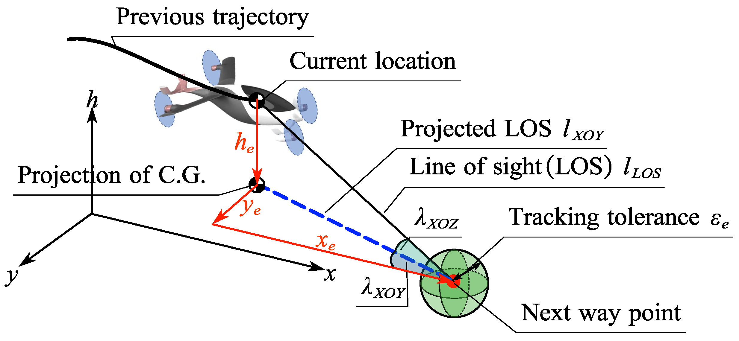
2.4. Performance Evaluation by Flight Guidance and Nonlinear Dynamic Inversion

2.4.1. Flight Guidance Law

As revealed by Section 2.1 and Section 2.2, it is of particular concern to investigate the performance merits of eVTOL in a long timescale. For an urban airspace with extensive non-fly zones, an obstacle-free reference trajectory is necessary to further analyze the performance. In this paper, we assume that the reference trajectory is predefined by, for instance, the global search or numerical optimization methods [25]. On this basis, the flight guidance law is employed to steer the aircraft to desired way points (WP), thus, reflecting the flight performance. To this end, let us consider the guidance scenario in Figure 3, which illustrates the previous trajectory, current location of aircraft (measured by the position of C.G. with its projection in the horizontal plane), and the next desired WP. The purpose of flight guidance law is to generate suitable acceleration command so that the aircraft tracks the WP in proper order. To do this, the line of sight (LOS), which connects the current aircraft location and WP, is employed to generate suitable acceleration command. Let us define two LOS angles ${\lambda }_{XOZ}$ and ${\lambda }_{XOY}$ in Figure 3, where ${\lambda }_{XOZ}$ is the line-surface angle between LOS and the $x_{I}O{y}_I$ plane, and ${\lambda }_{XOY}$ is the angle between the projected LOS (in the horizontal plane) and the $x_I$-axis. The flight guidance law reads [31]

$$\begin{array}{ccc}\hfill a_y& =& N_{y}V{\dot{\lambda }}_{XOY}\hfill \end{array}$$

(44)

$$\begin{array}{ccc}\hfill a_z& =& N_{z}V{\dot{\lambda }}_{XOZ}\hfill \end{array}$$

(45)

where $N_y$ and $N_z$ are, respectively, the guidance gains in lateral and vertical directions, and $a_y$ and $a_z$ are, respectively, the lateral and vertical acceleration command. Equations (44) and (45) imply that the longitudinal acceleration $a_x$ is desired to be zero along the flight.

To compute the time derivative of ${\lambda }_{XOZ}$ and ${\lambda }_{XOY}$, we further define the tracking errors as

$$\begin{array}{ccc}\hfill x_e& =& x-x_i^{*}\hfill \end{array}$$

(46)

$$\begin{array}{ccc}\hfill y_e& =& y-y_i^{*}\hfill \end{array}$$

(47)

$$\begin{array}{ccc}\hfill h_e& =& h-h_i^{*}\hfill \end{array}$$

(48)

where ${\left[x_i^{*},y_i^{*},h_i^{*}\right]}^{\top }$ is the location of the i-th WP ($i=1,2,\dots ,n$), and ${\left[x_e,y_e,h_e\right]}^{\top }$ is the tracking error. As such, ${\lambda }_{XOZ}$ and ${\lambda }_{XOY}$ are represented as

$$\begin{array}{ccc}\hfill {\lambda }_{XOY}& =& arctan\frac{h_e}{\sqrt{x_e^2+y_e^2}}\hfill \end{array}$$

(49)

$$\begin{array}{ccc}\hfill {\lambda }_{XOZ}& =& arctan\frac{y_e}{x_e}\hfill \end{array}$$

(50)

Taking the first-order derivatives of Equations (49) and (50) regarding time yields

$$\begin{array}{ccc}\hfill \frac{\mathrm{d}{\lambda }_{XOY}}{\mathrm{d}t}& =& \frac{l_{XOY}^{2}Vsin\gamma -h_e\left(x_{e}Vcos\gamma cos\chi +y_{e}Vcos\gamma sin\chi \right)}{l_{XOY}{l}_{LOS}^2}\hfill \end{array}$$

(51)

$$\begin{array}{ccc}\hfill \frac{\mathrm{d}{\lambda }_{XOZ}}{\mathrm{d}t}& =& \frac{x_{e}Vcos\gamma sin\chi -y_{e}Vcos\gamma cos\chi }{l_{XOY}^2}\hfill \end{array}$$

(52)

where $l_{LOS}$ and $l_{XOY}$ are, respectively, the length of LOS and its projection in the $x_{I}O{y}_I$ plane, given by

$$\begin{array}{ccc}\hfill l_{LOS}& =& \sqrt{x_e^2+y_e^2+h_e^2}\hfill \end{array}$$

(53)

$$\begin{array}{ccc}\hfill l_{XOY}& =& \sqrt{x_e^2+y_e^2}\hfill \end{array}$$

(54)

The desired WPs are given as a $3\times n$ matrix $\mathbf{W}$, that is,

$$\mathbf{W}\triangleq \left[\begin{array}{cccc}{x}_1^{*}& x_2^{*}& \dots & x_n^{*}\\ y_1^{*}& y_2^{*}& \dots & y_n^{*}\\ h_1^{*}& h_2^{*}& \dots & h_n^{*}\end{array}\right]\in {\mathbb{R}}^{3\times n}$$

(55)

where n is the number of WPs. The flight guidance law in Equations (44)–(54) is repeatedly called to track a series of WPs in Equation (55). To this effect, the desired WP should be switched to the next one where necessary. Herein, a predefined tracking tolerance ${\epsilon }_e$ is introduced. The index of WP is increased by one if the total tracking error, as measured by $l_{LOS}$, is smaller than ${\epsilon }_e$. A pseudocode of the guidance law is depicted in Algorithm 1. It is worth noting that the simulation is terminated when SOC reaches the lower bound of 0.2 considering the flight safety requirement. Herein, the simulation being terminated simply implies stopping the simulation and recording all the data so far, as this paper focuses on the aircraft performance evaluation. In practical implementations, suitable measures such as emergency landing should be taken before low SOC is reached.

Algorithm 1 Flight guidance law with switching way points

Input:  Way point sequence $\mathbf{W}\in {\mathbb{R}}^{3\times n}$, Tracking tolerance ${\epsilon }_e$, Guidance gains $N_y,N_z$, Aircraft location ${\left[x,y,h\right]}^{\top }$ and velocity V Output:  Commanded aircraft acceleration $a_y,a_z$  1: Initialization $i\leftarrow 1$  2: while  $i\le n$  do  3:    Get positional error $x_e,y_e,h_e$               ⊳ Equations (46)–(48)  4:    Get synthetic tracking error $l_{XOY},l_{LOS}$          ⊳ Equations (53) and (54)  5:    Compute the time derivatives of ${\lambda }_{XOY},{\lambda }_{XOZ}$       ⊳ Equations (51) and (52)  6:    Get line-of-sight angle                   ⊳ Equations (46)–(48)  7:    Generate the commanded acceleration $a_y,a_z$        ⊳ Equations (44) and (45)  8:    if $l_{LOS}$ < ${\epsilon }_e$ then  9:          $i\leftarrow i+1$ 10:    end if 11:    if $\mathrm{SOC}$ < 0.2 then 12:        break;                 ⊳ Considering safety flight requirements 13:    end if 14: end while 15: return $a_y,a_z$

2.4.2. Control Input Propagation by Nonlinear Dynamic Inversion

To evaluate the aircraft performance, the commanded acceleration generated by the flight guidance law presented in Section 2.4.1 should be further converted to the allowable control inputs $\alpha$, $\mu$, and ${\omega }_C$. The basic idea of this part is to implement the nonlinear dynamic inversion (NDI) to obtain the control inputs based on $a_y$ and $a_z$.

For brevity, the crude dynamics of electric propulsion are simplified subject to the following simplification

• Quasi-static assumption of electric propulsion. The time constants of electric propulsive states ${\omega }_E$ and $I_M$ are much smaller than that of rigid-body motions, for which the time derivatives of the former may be neglected, thus, giving rise to

  $${\dot{\omega }}_E={\dot{\omega }}_M={\dot{I}}_M\equiv 0$$

  (56)
• Following the previous point, the tuning process of the motor controller is omitted, the actual rotational speed is, thus, the same as the commanded value

  $${\omega }_M={\omega }_C$$

  (57)

It is noteworthy that the thermal dynamics and aging effect are not incorporated in the linearized model but rather taken as observed variables to showcase the influence of extreme and uncertain flight conditions. $Q_B$ and $U_P$ are retained as state variables since they are connected to energy consumption and LIB polarization, which are observed in a long timescale. Substituting Equations (56) and (57), respectively, into (14) and (15) leads to the quasi-static ECM of the motor, that is,

$$\begin{array}{ccc}\hfill I_M& =& {\displaystyle \frac{C_Q\rho {\left({\displaystyle \frac{{\omega }_C}{2\pi }}\right)}^2{D}_P^5}{K_T}}\hfill \end{array}$$

(58)

$$\begin{array}{ccc}\hfill U_M& =& I_M{R}_M+K_E{\omega }_C\hfill \end{array}$$

(59)

The resultant state, control, and output variables are defined as

$$\begin{array}{ccc}\hfill \tilde{\mathit{x}}& =& {\left[x,y,h,V,\chi ,\gamma ,Q_B,U_P\right]}^{\top }\hfill \end{array}$$

(60)

$$\begin{array}{ccc}\hfill \tilde{\mathit{u}}& =& {\left[\alpha ,\mu ,{\omega }_C\right]}^{\top }\hfill \end{array}$$

(61)

$$\begin{array}{ccc}\hfill \tilde{\mathit{y}}& =& {\left[I_M,U_M\right]}^{\top }\hfill \end{array}$$

(62)

During flight, it is expected that the longitudinal velocity of aircraft does not vary significantly, i.e., $a_x=0$. The desired equations of motion, adapted from Equations (4)–(6), read as

$$\begin{array}{ccc}\hfill 0& =& {\displaystyle \frac{T-D}{m}}-gsin\gamma \hfill \end{array}$$

(63)

$$\begin{array}{ccc}\hfill a_y& =& {\displaystyle \frac{Lsin\mu }{mcos\gamma }}\hfill \end{array}$$

(64)

$$\begin{array}{ccc}\hfill a_z& =& {\displaystyle \frac{Lcos\mu }{m}}-gcos\gamma \hfill \end{array}$$

(65)

Combining Equations (64) and (65) yields

$$\mu =arctan{\displaystyle \frac{a_{y}cos\gamma }{a_z+gcos\gamma }}$$

(66)

Substituting Equation (66) into (64) gives rise to the required lift as

$$L=\frac{m{a}_{y}cos\gamma }{sinarctan{\displaystyle \frac{a_{y}cos\gamma }{a_z+gcos\gamma }}}$$

(67)

To acquire the $\alpha$ value that provides the required lift, $C_L$ and $C_D$ in Equation (10) are approximated by [21]

$$\begin{array}{ccc}\hfill C_L& =& C_{L0}+C_{L\alpha }\alpha \hfill \end{array}$$

(68)

$$\begin{array}{ccc}\hfill C_D& =& C_{D0}+k{C}_L^2\hfill \end{array}$$

(69)

where $C_{L0}$ is the lift coefficient with zero angle of attack, $C_{L\alpha }$ is the lift-curve slope, $C_{D0}$ is the drag coefficient with zero lift, and k is the lift-induced drag factor.

By inverting Equations (10), (68) and (69) the required angle of attack is given by

$$\alpha =\frac{1}{C_{L\alpha }}\left(\frac{2mg}{\rho V^2{S}_{ref}cosarctan{\displaystyle \frac{a_{y}cos\gamma }{a_z+gcos\gamma }}}-C_{L0}\right)$$

(70)

On this basis, the aerodynamic drag is given by

$$D=\frac{1}{2}\rho V^2{S}_{ref}\left[C_{D0}+k{\left(\frac{2mg}{\rho V^2{S}_{ref}cosarctan{\displaystyle \frac{a_{y}cos\gamma }{a_z+gcos\gamma }}}\right)}^2\right]$$

(71)

which is counterbalanced by the total thrust. Hence, the required thrust of single propeller is determined by

$$T={\displaystyle \frac{{\displaystyle \frac{1}{2}}\rho V^2{S}_{ref}\left[C_{D0}+k{\left({\displaystyle \frac{2mg}{\rho V^2{S}_{ref}cosarctan{\displaystyle \frac{a_{y}cos\gamma }{a_z+gcos\gamma }}}}\right)}^2\right]+mgsin\gamma }{N_T}}$$

(72)

The left-hand side of Equation (72) is given by combining Equations (22) and (24), that is,

$$T=\left[C_{t2}{\left(\frac{2\pi Vcos\alpha }{{\omega }_C{D}_P}\right)}^2+C_{t1}\left(\frac{2\pi Vcos\alpha }{{\omega }_C{D}_P}\right)+C_{t0}\right]\rho {\left(\frac{{\omega }_C}{2\pi }\right)}^2{D}_P^4$$

(73)

${\omega }_C$ is thereby solved by combining Equations (72) and (73). With $\alpha$, $\mu$, ${\omega }_C$, and the initial states, it is possible to use numerical simulation to evaluate the aircraft performance subject to various uncertainties.

3. Results

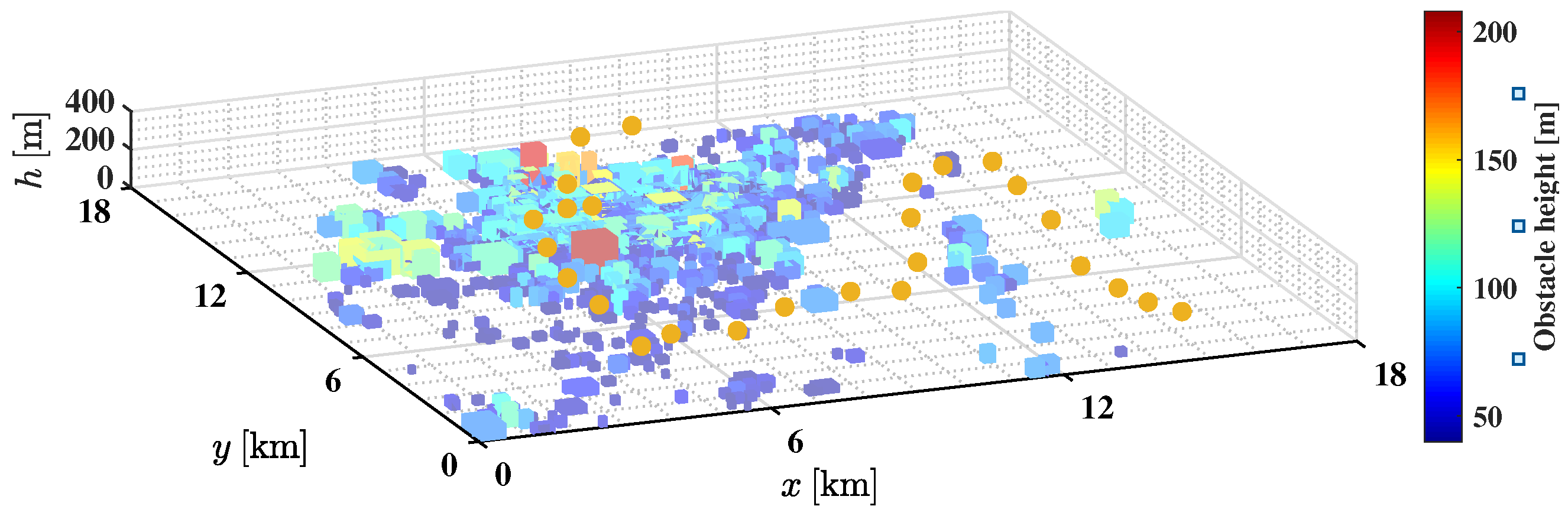
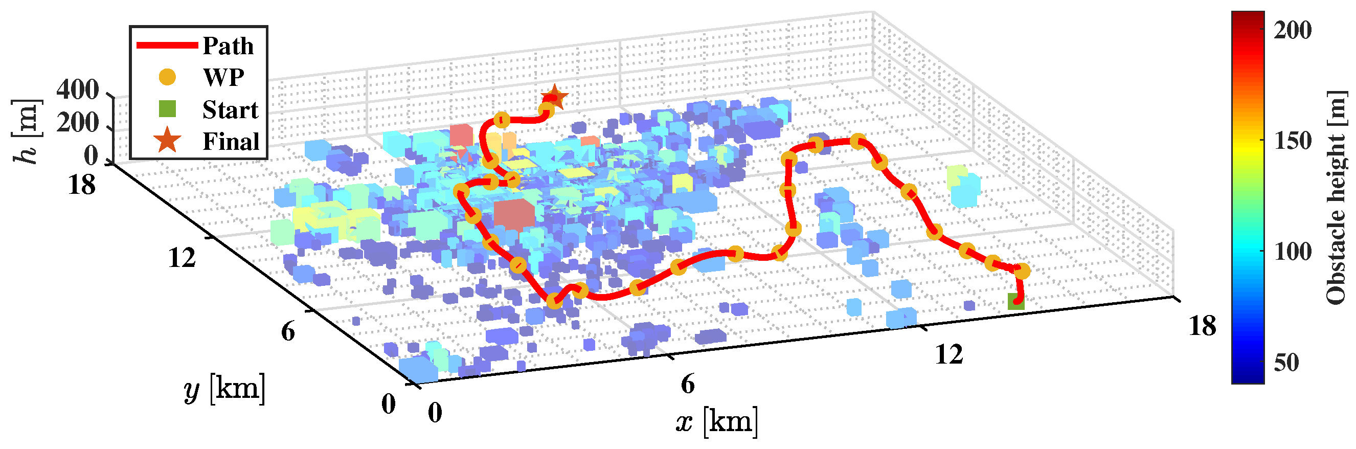
3.1. Exemplary Aircraft and Scenario

An exemplary eVTOL with six propellers is used to investigate the performance of electric flight in urban environments subject to changing ambient conditions and uncertainties. The primary parameters of the exemplary eVTOL are displayed in

Table 1. Primary parameters of the eVTOL aircraft test-bench ¹.

Parameter	Value	Parameter	Value 2
m	$380\mathrm{kg}$	$S_{ref}$	$6{\mathrm{m}}^2$
$D_P$	$0.55\mathrm{m}$	$Q_{max,nom}$	$3.45\mathrm{Ah}$
$R_P$	$1.27\times {10}^{-4}\Omega$	$C_P$	$198.61\mathrm{F}$
$R_B$	$0.0269\Omega$	$K_E$	$0.1042\mathrm{V}/(\mathrm{rad}/\mathrm{s})$
$K_T$	$0.1042\mathrm{Nm}/\mathrm{A}$	$R_M$	$0.0226\Omega$
$\left[c_{t2},c_{t1},c_{t0}\right]$	$\left[-0.2028,0.0498,0.1589\right]$	$\left[c_{q2},c_{q1},c_{q0}\right]$	$\left[-0.0343,0.0246,0.0131\right]$
${\omega }_{max}$	$650\mathrm{rad}/\mathrm{s}$	$S_B$	$3.68\times {10}^{-3}{\mathrm{m}}^2$
$h_c$	$90\mathrm{W}/\mathrm{K}{}^2$	$C_B$	$4000\mathrm{J}/\left(\mathrm{kg}·\mathrm{K}\right){}^2$

¹ The battery data are acquired using the test methods in Ref. [14]. ² The nominal values for batteries are tested at 25 $°\mathrm{C}$ [27].

. The crude size of the urban environment is enlarged by three times to represent a wide range of scenarios (See Figure 4).

The lift and drag coefficients in Equation (10) are represented as functions of $\alpha$ (in degree), that is,

$$\begin{array}{cc}\hfill C_L& =0.3521+0.08215\alpha \hfill \end{array}$$

(74a)

$$\begin{array}{cc}\hfill C_D& =0.03175+0.0028C_L+0.03586C_L^2\hfill \end{array}$$

(74b)

The street and building information of the New York Brooklyn borough [32] are adapted and scaled to represent a typical urban operational scenario. Specifically, each building is modeled as a cuboid with accurate latitude, longitude, and number of floors. It is assumed that the average height of each floor is 2m.

The wind speed distribution of the selected urban scenario is generated using the MATLAB© R2019b function “atmoshwm” [33], which outputs the wind speed with the given location (i.e., latitude, longitude, and altitude) and time (i.e., day of the year and time of day). Three typical altitude values $h=0,2,$ and $4\mathrm{km}$ and four day values (No. 1, 91, 181, and 301 to represent winter, spring, summer, and autumn) are used to showcase the wind speed characteristics. As shown in Figure 5, the changes in $V_{Wx}$ and $V_{Wy}$ due to different latitude and longitude are small enough compared to those led by altitude variation and, thus, omitted, which verifies the assumption of Equations (37) and (38). Comparing the illustrative vectors in the same altitude among Figure 5a–d implies that the wind direction may also change considerably due to different seasons, especially at low altitude ($h=0\mathrm{km}$) between January (almost aligned with the north) and April ($60°$ north by east). Moreover, the wind speed may also change within a day subject to different hours, as shown in Figure 6.

The change in urban ambient temperature in a day with respect to hours is generated by the urban weather generator [29]. Specifically, four typical days including the first day of January, April, July, and November are considered, as shown in Figure 7.

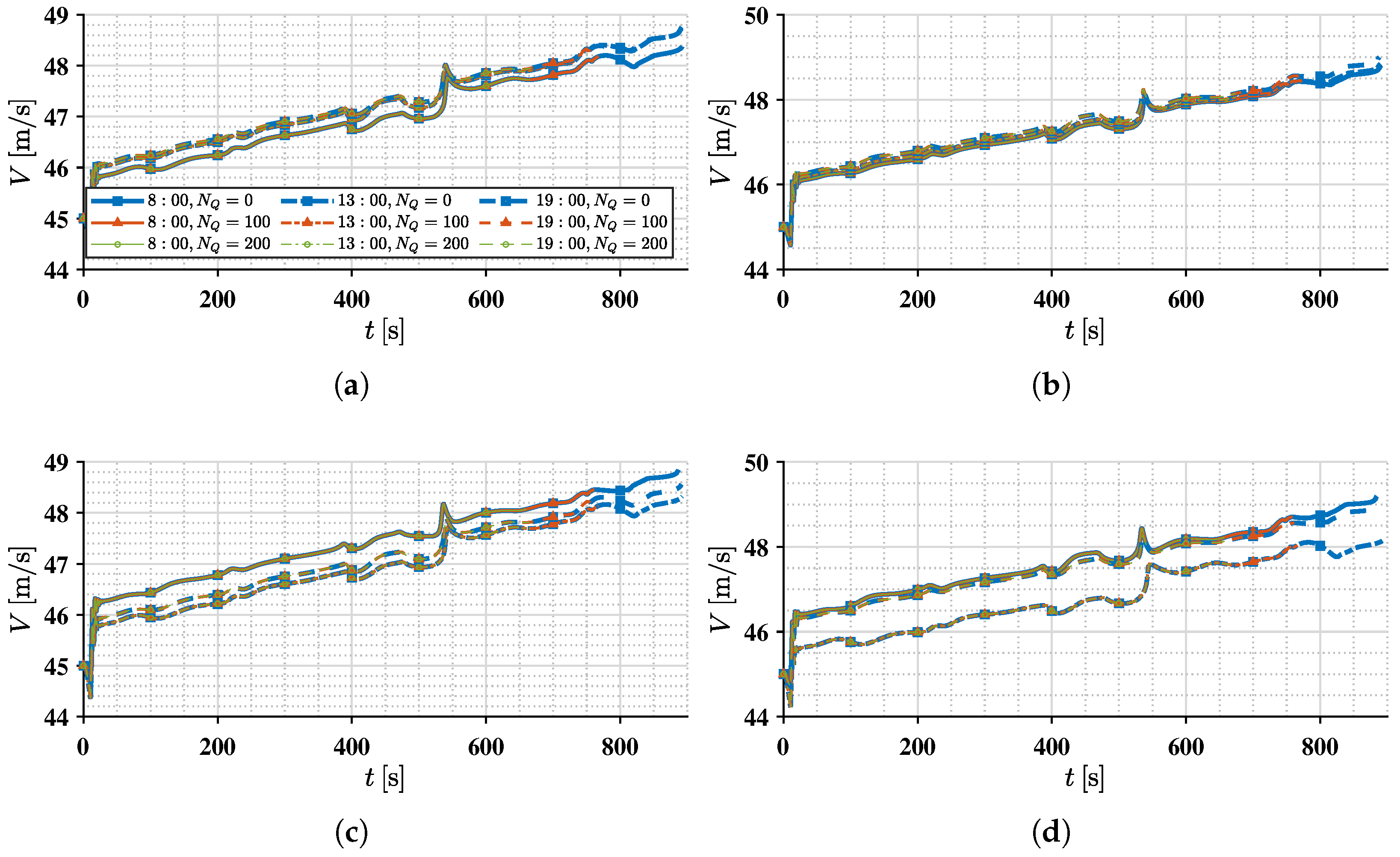
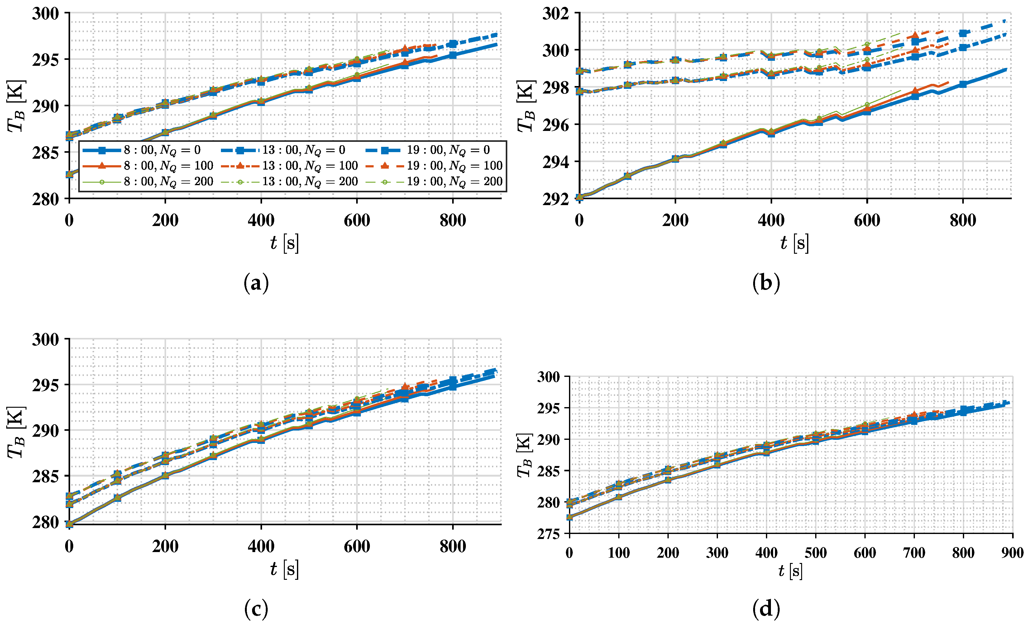
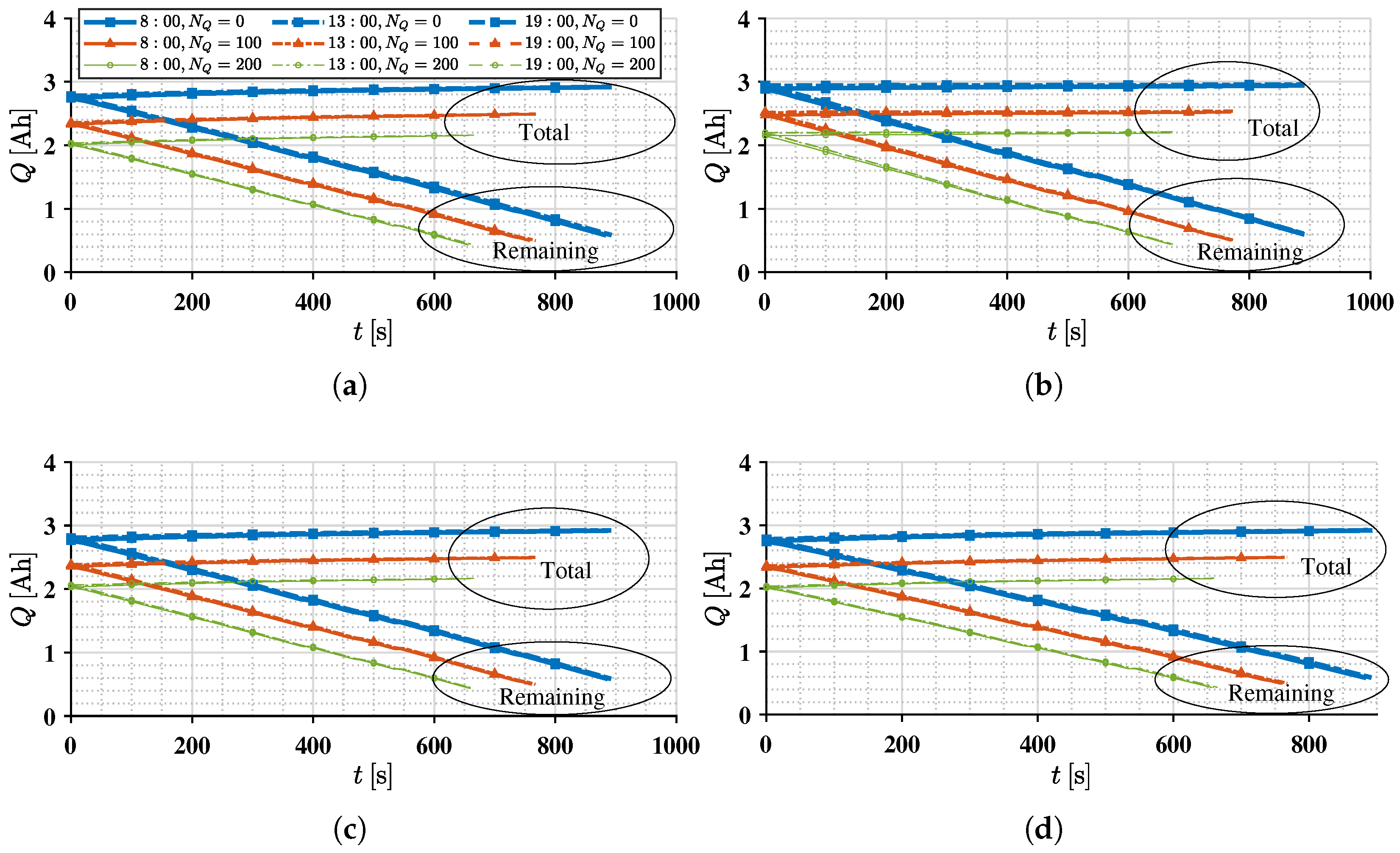
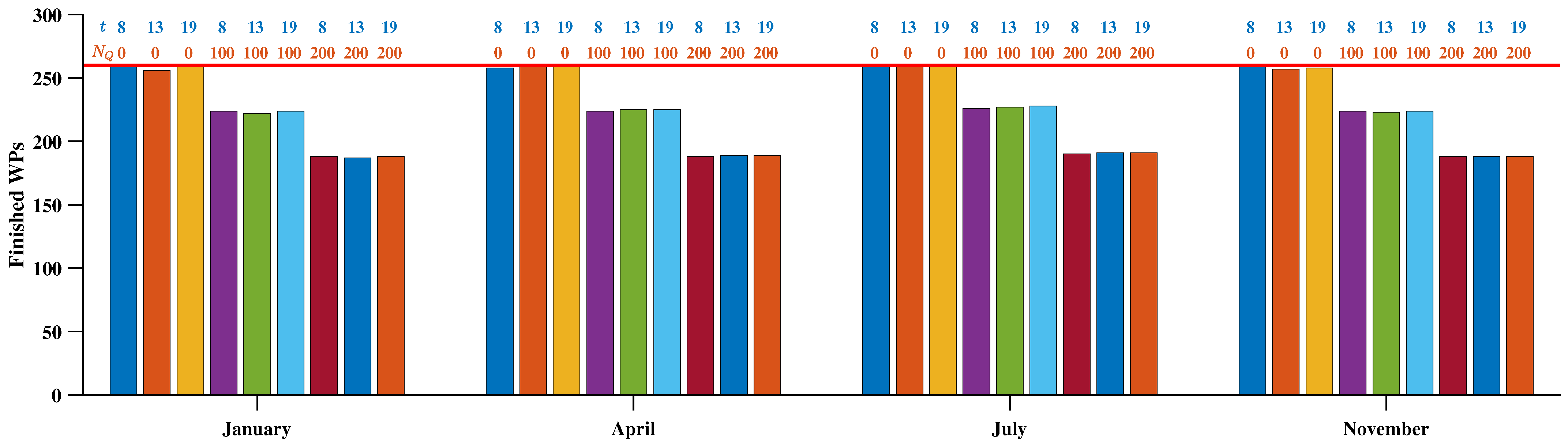
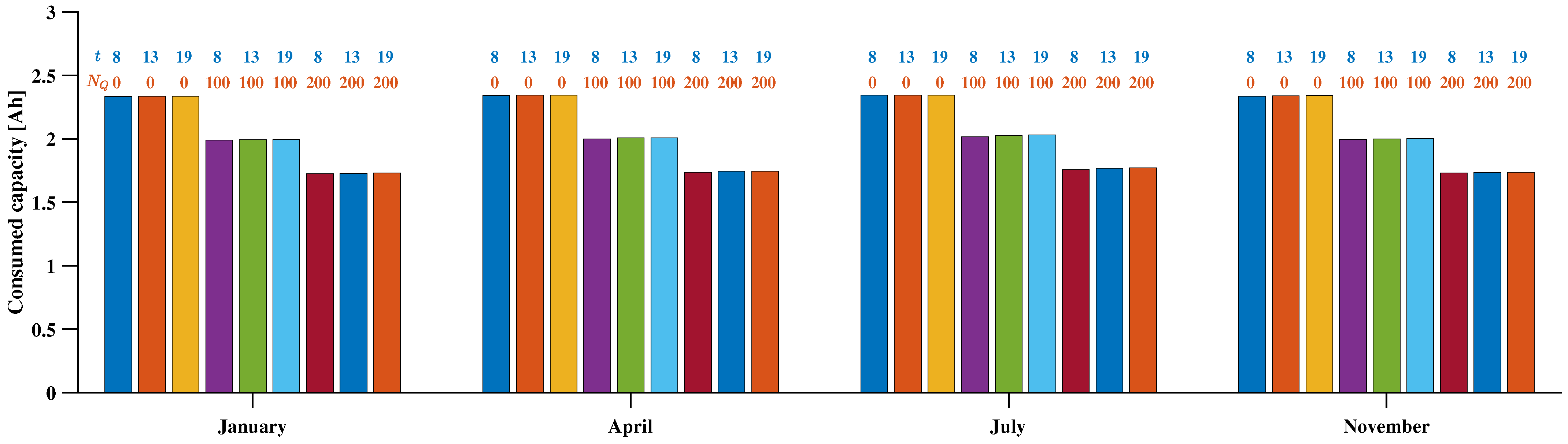
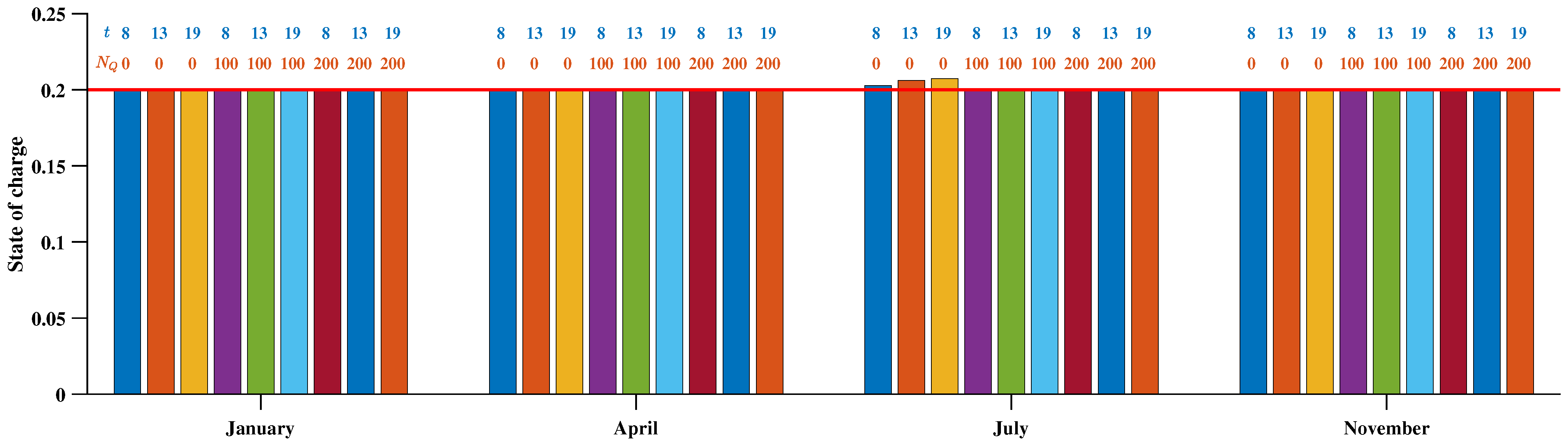
3.2. Simulation Results and Analysis

Based on the environmental data prepared in Section 3.1, the exemplary eVTOL is tested under various conditions, which include,

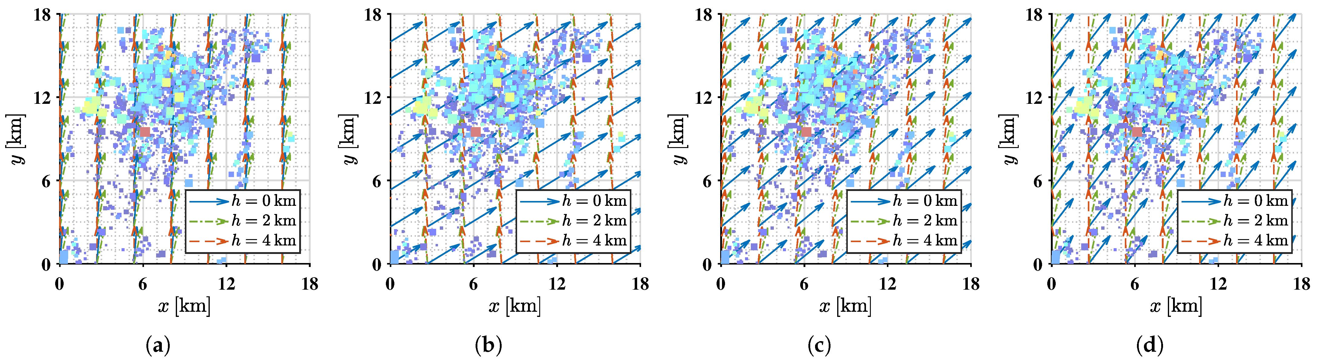
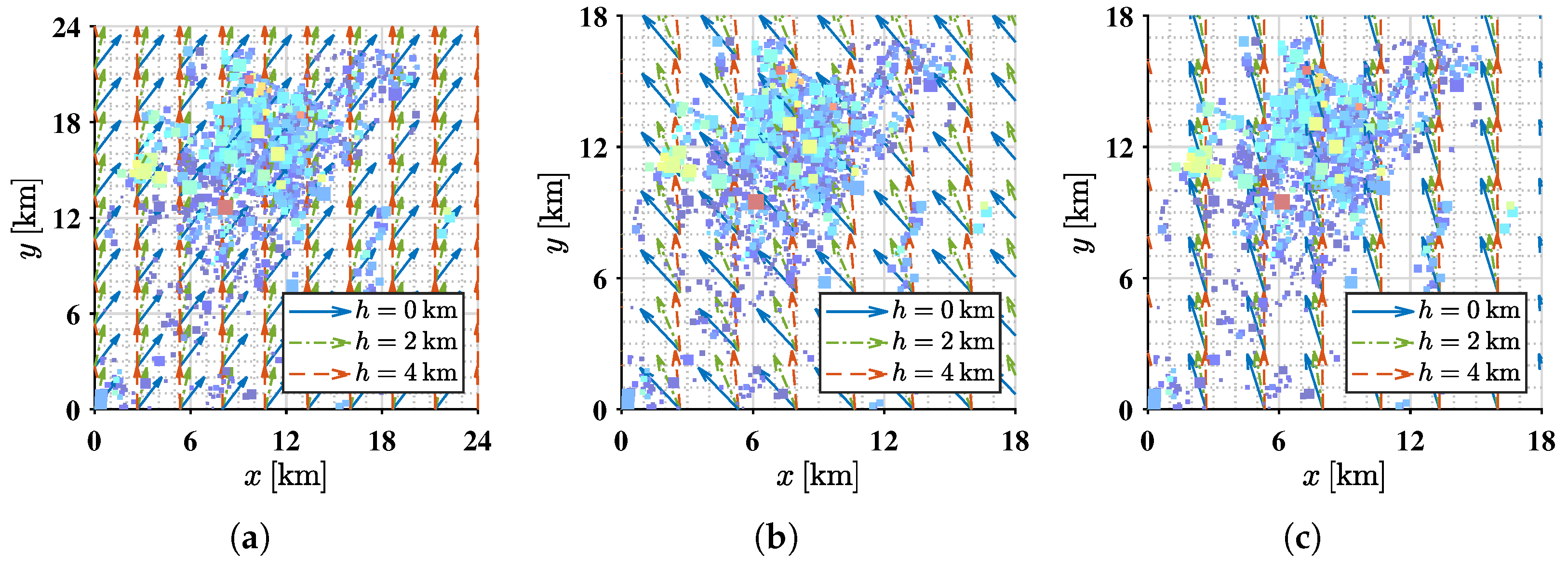
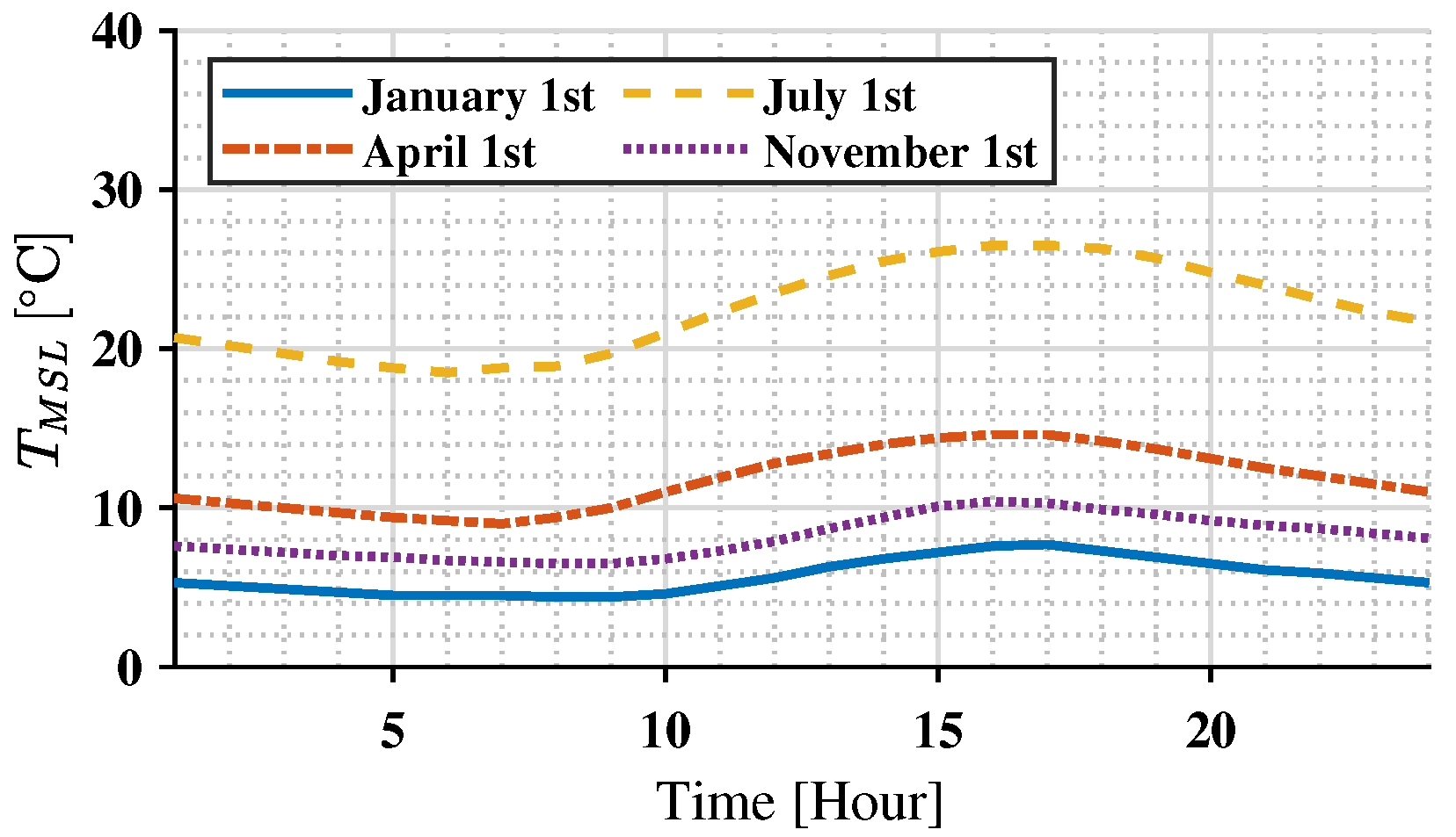
• Seasons represented by the month: January, April, July, and November.
• Time of day: 8:00, 13:00, and 19:00.
• Cycling numbers of LIBs: 0 (new batteries), 200, and 400.

Figure 8 showcases one of the tracking results of the predefined WPs with the condition being 1 April, 8:00, and a cycling number of 0. With the proposed guidance method, the aircraft passes through all the WPs as desired. This also holds true for the rest of the simulation cases. Thus, the focus of this part is placed on the influence of aircraft performance change led by the uncertain environment.

The time series of aircraft velocity V are illustrated in Figure 9. During flight, there is a slight increase in V from $45\mathrm{m}/\mathrm{s}$ to about $49\mathrm{m}/\mathrm{s}$, which implies that the imposed constraint of $a_x=0$ by Equations (44) and (45) is to a large extent fulfilled. It can be observed that with a higher basic $T_{MSL}$, the variation in V during flight is decreased. Specifically, in Figure 9b, which represents the summer, the variation in V is less than $0.5\mathrm{m}/\mathrm{s}$. In comparison, the maximum variation in V in Figure 9d is $1.1\mathrm{m}/\mathrm{s}$.

In contrast with the aircraft rigid-body performance, the battery temperature $T_B$ presents, nevertheless, an opposite pattern. In simulation, it is assumed that the initial temperature of LIBs is the same as $T_{MSL}$. Specifically, $T_{MSL}$ on 1 July (as indicated by Figure 10b) is at least $292\mathrm{K}$, corresponding to 8:00 in the morning. In the other cases of Figure 10b, the initial values of $T_B$ are even higher at 13:00 and 19:00 ($297.5\mathrm{K}$ and $299\mathrm{K}$, respectively) due to the urban heat island effect. On the contrary, the lower ambient temperature is beneficial for a more stable $T_B$, as indicated by Figure 10d.

The influence of the LIB aging effect is investigated in Figure 11 by comparing the maximum and remaining battery capacities, with the latter defined as $Q_{max}-Q_B$. In each subfigure, the maximum capacity $Q_{max}$ is represented using the same line style corresponding to the remaining capacity. A significant decrease in $Q_{max}$ due to the aging effect is observed in all the simulation cases. Despite the difference in battery temperature, which also changes $Q_{max}$ according to the thermal effect of Equation (30), the increase in cycling number $N_Q$ is a dominant factor that leads to the uncertainty in $Q_{max}$. In the simulation cases, $Q_{max}$ is decreased on average by $0.4\mathrm{Ah}$ when $N_Q$ is increased from 0 to 100 and by $0.3\mathrm{Ah}$ when $N_Q$ further grows to 200. It is noteworthy that, as a result, not all the missions are finished owing to the loss of $Q_{max}$.

To this end, the mission completion and energy consumption are plotted as bars in Figure 12, Figure 13 and Figure 14. The results are also quantitatively compared in

Table 2. Simulation results under different conditions.

Date	Time	${\mathit{N}}_{\mathit{Q}}$	Finished WPs	SOC 1	${\mathit{Q}}_{\mathit{B}}\left[\mathbf{Ah}\right]{}^1$
1 January	8:00	0	260	0.2000	2.3329
		100	224	0.2000	1.9903
		200	188	0.2000	1.7244
	13:00	0	256	0.2000	2.3357
		100	222	0.2000	1.9937
		200	187	0.2000	1.7282
	19:00	0	260	0.2000	2.3365
		100	224	0.2000	1.9949
		200	188	0.2000	1.7299
1 April	8:00	0	258	0.2000	2.3401
		100	224	0.2000	1.9994
		200	189	0.2000	1.7244
	13:00	0	260	0.2000	2.3452
		100	225	0.2000	2.0068
		200	189	0.2000	1.7442
	19:00	0	260	0.2000	2.3402
		100	225	0.2000	2.0073
		200	189	0.2000	1.7362
1 July	8:00	0	260	0.2028	2.3447
		100	226	0.2000	2.0161
		200	190	0.2000	1.7554
	13:00	0	260	0.2073	2.3392
		100	227	0.2000	1.9980
		200	191	0.2000	1.7337
	19:00	0	260	0.2062	2.3402
		100	228	0.2000	2.0313
		200	191	0.2000	1.7362
1 November	8:00	0	260	0.2000	2.3358
		100	224	0.2000	1.9942
		200	188	0.2000	1.7290
	13:00	0	257	0.2000	2.3392
		100	223	0.2000	1.9980
		200	188	0.2000	1.7337
	19:00	0	258	0.2000	2.3402
		100	224	0.2000	2.0000
		200	188	0.2000	1.7362

¹ $\mathrm{SOC}$$Q_B$ are both the terminal values at the end of simulation.

. Therein, each bar is accompanied by the corresponding time (i.e., 8:00, 13:00, and 19:00) and $N_Q$ (i.e., 0, 100, 200), and the simulation results are grouped by month. It is observed that the number of finished WPs can change by at most 1.53% due to the time of day (i.e., 1 January, finished WPs reduced from 260 to 256 when time changed from 8:00 to 13:00). In 1 July, when the mean-sea-level temperature is higher, the number of finished WPs presents the least variation in all battery aging status (i.e., at most change by 1). Aging is proven to be the most significant factor that influences the aircraft performance. The initial value of $Q_{max}$ is separately reduced by 15.05% and 26.68% with $N_Q$ increasing from 0 to 100 and 200 on 1 January. In comparison, the weather condition in 1 July enables higher robustness against the aging status, where $Q_{max}$ drops, respectively, by 14.18% and 25.16% with $N_Q=100$ and $N_Q=200$. With $N_Q=0$, the missions in all cases are to a large extent finished. There are two expectations at 13:00 for 1 January and 1 November, where the number of the finished WPs are separately 256 and 257. This phenomenon can be interpreted by the lower $T_{MSL}$ in these two months compared to the other two, which leads to a lower initial battery temperature and, thus, the lower $Q_{max}$ due to the thermal effect.

For the selected scene and mission, the final SOC of the exemplary aircraft reaches the lower bound of 0.2, except for the cases in 1 July with $N_Q=0$, regardless of time of day. The underlying reason is also attributed to the better battery performance due to the higher ambient temperature in summer.

4. Discussion

Based on the simulation results and analysis, the following observations and suggestions on urban electric flight in the selected area may be drawn.

• For the selected operating scene, the performance of the exemplary aircraft is more sensitive to the battery aging effect compared to the other uncertainties of weather, the urban heat island effect, and wind. Thus, it is necessary to pay attention to the cycling number of LIBs used in the electric aircraft.
• Given the premise that the LIB temperature stays below the safety value, it is beneficial to operate electric aircraft with a higher ambient temperature, for instance, in summer, and make use of the urban heat island effect.
• The change in time of day results in different mean-sea-level temperatures and wind directions. For the operating range of urban electric flight, the magnitude of wind speed may be considered as constant regardless of the latitude and longitude change. However, the wind speed variation (especially the wind direction) as a result of different altitudes should be incorporated.

The results of this paper are further compared to the conclusions drawn in [20]. The benchmark study in several typical U.S. cities implies that the most favorable environmental condition turns out to be along the Californian coast, as opposed to the other cities with higher latitudes such as Denver, New York, and Washington D.C. This coincides with the findings in this paper that a higher mean-sea-level temperature and weaker vertical wind shear are beneficial to urban electric flight.

The current study can be enriched in the future by the following aspects.

• Models of electric propulsion systems with higher fidelity. Currently, the thermal dynamics of the battery pack are represented by the lumped-parameter model of a single LIB cell. This can be improved by introducing a more accurate pack model considering the heat transfer among cells. Furthermore, the motor thermal dynamics and effect are not considered so far. Necessary constraints should be incorporated in future works.
• Dynamic aging model of LIB. In this paper, the aging condition of LIBs is directly specified by setting cycling numbers. In actuality, the aging process of an LIB can be complex due to different mission loads and usage conditions. Hence, more precise aging models need to be employed to dynamically evaluate the aging status of the LIB.
• Four-dimensional guidance. In this work, the velocity is desired to be constant during flight. In real-world operations, it is often the case to set a desired arrival time in UAM. Therefore, the current guidance law can be updated to accommodate this requirement.

5. Conclusions

This paper investigates electric flight under extreme and uncertain urban environments. A three-dimensional point-mass model of an electric aircraft is developed. The internal uncertainties, including the thermal and aging effect, together with the external uncertainties, including the wind, the urban heat island effect, and the change in seasons, are modeled therewith. A performance evaluation method based on guidance law and nonlinear dynamic inversion is proposed to study the influence of these uncertainties on the aircraft performance. The findings are as follows

• The proposed flight guidance law is applicable for electric aircraft to realize way-point tracking in various urban scenes, despite the internal and external uncertainties.
• Electric aircraft performance varies considerably with respect to the micro-climate in the urban environment. Among others, the change in mean-sea-level temperature led by different seasons or the urban heat island effect is the dominant factor to consider in analysis. The number of finished way points can change by at most 1.53% due to the time of day. When the mean-sea-level temperature is higher, the number of finished way points presents the least variation (no larger than 0.38%) in all battery aging statuses. The higher mean-sea-level temperature contributes to a lower fluctuation in aircraft velocity, yet leads to a higher accumulation rate in generated battery heat and, thus, a more quickly increasing battery temperature.
• The aging status of LIB, which results in the loss of maximum capacity, is an important internal uncertainty that causes degradation in the electric aircraft performance, especially in the maximum range. With a typical urban environment and load profile, the maximum battery capacity is separately reduced at most by 15.05% and 26.68% with cycling numbers of 100 and 200. Thus, the cycling number of LIB should be carefully monitored.

Considering the changing urban environment and battery aging status, further suggestions may be proposed with respect to the electric aircraft design. For instance, the sensitivity of interested performance merits (e.g., range and energy consumption) regarding uncertain parameters can be quantitatively acquired based on the forward sensitivity method. On this basis, it is feasible to perform a desensitized design optimization that is beneficial to reduce the performance variance led by uncertainties, thus, improving the design robustness.

In the present work, only lumped-parameter and equivalent-circuit models were employed to reflect the coupling relationships between the ambient uncertainties and the electric aircraft performance. Furthermore, the important aging effect is represented by the given cycling numbers instead of a gradually varying status subject to the real load profile. Therefore, future works will focus on improving the model fidelity in terms of both thermal and aging effects. Meanwhile, velocity control should be incorporated in the guidance law to achieve four-dimensional guidance.

References

1. Cohen, A.P.; Shaheen, S.A.; Farrar, E.M. Urban Air Mobility: History, Ecosystem, Market Potential, and Challenges. IEEE Trans. Intell. Transp. Syst. 2021, 22, 6074–6087. [Google Scholar] [CrossRef]
2. Thipphavong, D.; Apaza, R.; Barmore, B.; Battiste, V.; Burian, B.; Dao, Q.; Feary, M.; Go, S.; Goodrich, K.; Homola, J.; et al. Urban air mobility airspace integration concepts and considerations. In Proceedings of the 2018 Aviation Technology, Integration, and Operations Conference, Atlanta, GA, USA, 25–29 June 2018; pp. 1–20. [Google Scholar] [CrossRef]
3. Goyal, R.; Reiche, C.; Fernando, C.; Cohen, A. Advanced Air Mobility: Demand Analysis and Market Potential of the Airport Shuttle and Air Taxi Markets. Sustainability 2021, 13, 7421. [Google Scholar] [CrossRef]
4. Ullah, I.; Safdar, M.; Zheng, J.; Severino, A.; Jamal, A. Employing Bibliometric Analysis to Identify the Current State of the Art and Future Prospects of Electric Vehicles. Energies 2023, 16, 2344. [Google Scholar] [CrossRef]
5. Rothfeld, R.; Fu, M.; Balać, M.; Antoniou, C. Potential Urban Air Mobility Travel Time Savings: An Exploratory Analysis of Munich, Paris, and San Francisco. Sustainability 2021, 13, 2217. [Google Scholar] [CrossRef]
6. Zhang, J.; Jiang, T.; Liu, Y.; Zheng, Y. Multi-fidelity Optimization of Ducted Fan for eVTOL Aircraft. In Proceedings of the AIAA Aviation 2023 Forum, San Diego, CA, USA, 12–16 June 2023; pp. 1–10. [Google Scholar] [CrossRef]
7. Cavallo, A.; Cancielloa, G.; Russo, A. Buck-Boost Converter Control for Constant Power Loads in Aeronautical Applications. In Proceedings of the 2018 IEEE Conference on Decision and Control, Miami Beach, FL, USA, 12–16 June 2018; pp. 6741–6747. [Google Scholar] [CrossRef]
8. Wang, M.; Chu, N.; Bhardwaj, P.; Zhang, S.; Holzapfel, F. Minimum-Time Trajectory Generation of eVTOL in Low-Speed Phase: Application in Control Law Design. IEEE Trans. Aerosp. Electron. Syst. 2023, 59, 1260–1275. [Google Scholar] [CrossRef]
9. Russo, A.; Cavallo, A. Stability and Control for Buck–Boost Converter for Aeronautic Power Management. Energies 2023, 16, 988. [Google Scholar] [CrossRef]
10. Steiner, M. Urban Air Mobility: Opportunities for the Weather Community. Bull. Am. Meteorol. Soc. 2019, 100, 2131–2133. [Google Scholar] [CrossRef]
11. NASA. U.S. Standard Atmosphere; Technical Report; U.S. Government Printing Office: Washington, DC, USA, 1976.
12. Bradford, S. Urban Air Mobility (UAM) Concept of Operations; Technical Report; Federal Aviation Administration: Washington, DC, USA, 2020.
13. Avinor. Preferences for the Introduction of Electrified Commercial Aircraft; Technical Report; Civil Aviation Authority of Norway: Bodo, Norway, 2020. [Google Scholar]
14. Wang, M.; Luiz, S.O.D.; Lima, A.M.N. Desensitized Optimal Control of Electric Aircraft Subject to Electrical-Thermal Constraints. IEEE Trans. Transp. Electrif. 2022, 8, 4190–4204. [Google Scholar] [CrossRef]
15. Luiz, S.O.D.; Souza, E.G.; Lima, A.M.N. Representing the Accumulator Ageing in an Automotive Lead-Acid Battery Model. J. Control. Autom. Electr. Syst. 2022, 33, 204–218. [Google Scholar] [CrossRef]
16. Vermeer, W.; Mouli, G.R.C.; Bauer, P. A Comprehensive Review on the Characteristics and Modeling of Lithium-Ion Battery Aging. IEEE Trans. Transp. Electrif. 2022, 8, 2205–2232. [Google Scholar] [CrossRef]
17. Rezende, R.N. General Aviation Electrification: Challenges on the transition to new technologies. In Proceedings of the AIAA Propulsion and Energy 2021 Forum, Virtual Event, 9–11 August 2021; pp. 1–7. [Google Scholar]
18. Pintos, P.B.; Sande, C.U.; Álvarez, Ó.C. Sustainable propulsion alternatives in regional aviation: The case of the Canary Islands. Transp. Res. Part D 2023, 120, 103779. [Google Scholar] [CrossRef]
19. Bærheim, T.; Lamb, J.J.; Nøland, J.K.; Burheim, O.S. Potential and Limitations of Battery-Powered All-Electric Regional Flights—A Norwegian Case Study. IEEE Trans. Transp. Electrif. 2023, 9, 1809–1825. [Google Scholar] [CrossRef]
20. Reiche, C.; Cohen, A.P.; Fernando, C. An Initial Assessment of the Potential Weather Barriers of Urban Air Mobility. IEEE Trans. Transp. Electrif. 2021, 22, 6018–6027. [Google Scholar] [CrossRef]
21. Wang, M.; Zhang, S.; Shi, D.; Holzapfel, F. Operational availability analysis of short-haul electric aeroplane using polynomial chaos expansion. Transp. B Transp. Dyn. 2022, 10, 988–1009. [Google Scholar] [CrossRef]
22. Clarke, M.A.; Alonso, J.J. Forecasting the Operational Lifetime of Battery-Powered Electric Aircraft. J. Aircr. 2023, 60, 47–55. [Google Scholar] [CrossRef]
23. Johnson, W.; Silva, C. Observations from Exploration of VTOL Urban Air Mobility Designs. In Proceedings of the 7th Asian/Australian Rotorcraft Forum, Jeju Island, Korea, 29 October–1 November 2018; pp. 1–15. [Google Scholar]
24. Stevens, B.L.; Lewis, F.L.; Johnson, E.N. The Kinematics and Dynamics of Aircraft Motion. In Aircraft Control and Simulation: Dynamics, Controls Design, and Autonomous Systems, 3rd ed.; John Wiley & Sons, Inc.: Hoboken, NJ, USA, 2016; pp. 1–44. [Google Scholar] [CrossRef]
25. Wang, M.; Zhang, S.; Diepolder, J.; Holzapfel, F. Battery Package Design Optimization for Small Electric Aircraft. Chin. J. Aeronaut. 2020, 33, 2864–2876. [Google Scholar] [CrossRef]
26. Bernardi, D.; Pawlikowski, E.; Newman, J. A General Energy Balance for Battery Systems. J. Electrochem. Soc. 1985, 132, 5–12. [Google Scholar] [CrossRef]
27. Panasonic Industry. Specifications for NCR18650GA, 1st ed.; Panasonic Industry Co., Ltd.: Secaucus, NJ, USA, 2017. [Google Scholar]
28. Bueno, B.; Norford, L.; Hidalgo, J.; Pigeon, G. The urban weather generator. J. Build. Perform. Simul. 2013, 6, 269–281. [Google Scholar] [CrossRef]
29. Yang, J.H. The Curious Case of Urban Heat Island: A Systems Analysis. Ph.D. Thesis, Massachusetts Institute of Technology, Cambridge, MA, USA, 2016. [Google Scholar]
30. Weitz, L.A. Derivation of a Point-Mass Aircraft Model Used for Fast-Time Simulation; Technical Report; MITRE Company: Bedford, MA, USA, 2015. [Google Scholar]
31. Zarchan, P. Trajectory Shaping Guidance. In Tactical and Strategic Missile Guidance, 6th ed.; American Institute of Aeronautics and Astronautics: Reston, VA, USA, 2012; pp. 569–600. [Google Scholar] [CrossRef]
32. New York City Department of City Planning. PLUTO and MapPLUTO. Available online: https://www.nyc.gov/site/planning/data-maps/open-data/dwn-pluto-mappluto.page (accessed on 27 June 2023).
33. Mathworks. Atmoshwm: Implement Horizontal Wind Model; The MathWorks: Natick, MA, USA, 2019; Available online: https://ww2.mathworks.cn/help/aerotbx/ug/atmoshwm.html (accessed on 25 June 2023).
Figure 1. Force equilibrium and frames of the eVTOL dynamic model.
Sustainability 15 12590 g001
Figure 2. Diagram of the proposed simulation model.
Sustainability 15 12590 g002
Figure 3. Considered guidance scenario of electric aircraft.
Sustainability 15 12590 g003
Figure 4. Scaled urban operational scenario with WPs (denoted by round circles).
Sustainability 15 12590 g004
Figure 5. Wind speed distribution of the selected scenario at different altitude and days. (a) Day 1. (b) Day 91. (c) Day 181. (d) Day 301.
Sustainability 15 12590 g005
Figure 6. Wind speed distribution of the selected scenario at different altitude and hours on Day 301. (a) 8:00. (b) 13:00. (c) 19:00.
Sustainability 15 12590 g006
Figure 7. Urban ambient temperature change with respect to hours in a day.
Sustainability 15 12590 g007
Figure 8. Actual trajectory of the exemplary following the predefined WPs.
Sustainability 15 12590 g008
Figure 9. Time series of velocity in different simulation conditions. (a) 1 April. (b) 1 July. (c) 1 November. (d) 1 January.
Sustainability 15 12590 g009
Figure 10. Time series of battery cell temperature in different simulation conditions. (a) 1 April. (b) 1 July. (c) 1 November. (d) 1 January.
Sustainability 15 12590 g010
Figure 11. Time series of total and remaining battery capacity in different simulation conditions. (a) 1 April. (b) 1 July. (c) 1 November. (d) 1 January.
Sustainability 15 12590 g011
Figure 12. Number of finished WPs vs. total WPs (denoted by the horizontal solid line).
Sustainability 15 12590 g012
Figure 13. Consumed capacity.
Sustainability 15 12590 g013
Figure 14. Final vs. minimum (denoted by the horizontal solid line) state of charge.
Sustainability 15 12590 g014