Experimental and Numerical CFD Modelling of the Hydrodynamic Effects Induced by a Ram Pump Waste Valve

Abstract

The hydraulic ram pump or hydram is a machine capable of lifting water to a hydraulic head higher than the level of the supply source. It is a sustainable and self-sufficient device: the working principle is based on the rise of abrupt pressure variations occurring in the feeding pipeline when the liquid inside it undergoes a locally sharp change in velocity as a consequence of the sudden closure of the waste valve. Invented in 1772, the pump has been improved over the decades. Due to its simplicity, low cost and reliability, it has been widely used worldwide to provide adequate domestic water supplies, especially before the spreading of electricity and internal combustion engines. In recent years, the new attention placed on sustainability and energy transition from fossil fuels to renewable energy devices has brought a growing interest to this basic machine, essentially forgotten and abandoned in the last century; it seems promising especially in developing countries. The hydram is, in fact, a very simple machine, with only two moving parts, the waste and delivery valves. The efficiency of the hydraulic ram pump is mainly influenced by the characteristics of the waste valve. However, sufficient data are not available for the design of the hydram and the waste valve. In this work, the behaviour of the waste valve of a hydram was simulated by means of Computational Fluid Dynamics (CFD). Velocity and pressure values were analysed for different scenarios with different closing times of the valve. The data obtained from the developed numerical model were compared, in order to verify the validity of the simulations, with those collected during the operation of the hydram placed at the Laboratory of Environmental and Marine Hydraulics (LIDAM) of the University of Salerno, Italy. The numerical model thus obtained can, therefore, be used to identify the ideal configuration of the valve in order to ensure the best performance of the hydram.

1. Introduction

1.1. The Hydraulic Ram Pump or Hydram

The hydraulic ram pump—commonly referred to as a hydram—is a machine that allows for lifting water to a hydraulic head higher than the level of the supply source, exploiting the kinetic energy of a moving water column and not other energy sources. It is, therefore, a sustainable and self-sufficient device, which is based on the development of pressure transients, occurring when the liquid inside the pump undergoes a sharp change in velocity generated by the sudden closure of the waste valve.

From the constructive point of view, the hydram is a basic yet robust machine, in which the only two moving parts are the waste and delivery valves (Figure 1). It is, therefore, a straightforward device, and as long as there is a permanent flow of water, the pump works continuously and automatically.

In the case that the fluid velocity in a pipe is high enough, its abrupt variation, consequent to the sudden closing of a waste valve, also determines a sudden increase in pressure (Figure 2), which, to a certain extent, can be compared to the well-known water hammer effect, since the water column is locally compressed by the closure of the valve. In fact, water flowing with a certain velocity has kinetic energy, and therefore a certain inertia, and the abrupt closure of the pipeline involves the transformation of this kinetic energy into pressure energy. This effect may turn into a loud noise similar to that of a hammer hitting a metal component.

Providing adequate domestic water supplies, especially for rural populations, is a major problem in developing countries and entails high maintenance and fuel consumption costs necessary for the operation of conventional pumping systems. The hydraulic ram has been used worldwide for over two centuries. Due to its simplicity and reliability, it was widely used mainly in Europe before the spreading of electricity and internal combustion engines. With technological advancement, developed countries have increasingly relied on primary energies derived from fossil fuels, and the hydram has been gradually forgotten and abandoned. However, in recent years, a growing interest in sustainability and the development of renewable energy devices has prompted the rediscovery of this technology, especially in developing countries. To use this technology, it is necessary to have a water source located at a higher altitude than that of the water pump, for example, a tank or a watercourse on a hill, which allows for the pump to be installed at a lower height.

Through a system of supply pipes, the water source is connected to the ram pump, which directs the flow through an internal system of valves that allows for increasing the pressure as a result of the water hammer, pumping the water through a delivery pipe.

A hydraulic ram pump has several goals:

• To raise water from a water source to a target community;
• To withstand external aggressions such as weather, rain, mud, organic matter, shocks, thefts and landslides;
• To withstand internal fatigue due to the impact of the water hammer effect.

The basic requirements needed to install and use a hydraulic ram pump are:

• A sufficient water source;
• A slope towards the pump;
• A physically possible high delivery in interaction with the headstock;
• A realistic amount of water to pump.

The main advantages of ram pumps are:

• The use of a renewable energy source that guarantees low running costs;
• The ability to pump only a small part of the available flow, with the possibility of returning the ejected water to the source, ensuring minimum environmental impact;
• Simplicity and reliability of the device and low maintenance requirements;
• Good potential for local production in rural villages;
• Automatic and continuous operation, not requiring human input.

The main limitations of this technology are:

• The pump is limited to hilly areas with water sources present all year round (the lack of an adequate water supply flow rate would result in an inevitable shutdown of the pump);
• It pumps only a small part of the available flow and, therefore, requires a much larger source capacity than the volume of water to be delivered;
• It can have a high design and installation cost compared to other technologies (especially in those countries where it is difficult to find the necessary components);
• It is generally limited to small-scale applications, typically up to 1KW, although technological progress has made it possible to design ram pumps with greater power.

1.2. Analysis of the Literature

Invented by Whitehust in 1772, and subsequently perfected by Montgolfier with the introduction of a pulse valve, the hydraulic ram pump has been the subject of studies conducted by numerous researchers from all over the world [1,2,3]. This research aims at defining a rational theory to analytically describe the behaviour of the pump in order to improve its performance through the optimal sizing of its main components. Among the numerous studies in the literature, some are dedicated to the analytical description of the pump’s behaviour, described with detailed and complex theory or simplified theory [4,5].

The mechanical engineer Krol carried out an in-depth and detailed study [6] regarding the automatic behaviour of the hydraulic ram, based on the subdivision of the entire operating cycle into seven periods, which allows for predicting the performance of a specific configuration of the pump after having deduced four parameters experimentally, including the pressure drops due to the waste valve. O’Brien and Gosline [7], instead, describe the operating cycle of the hydraulic ram pump through four main time periods. Basfeld and Miiller [8] described the behaviour of the pump with a simplified theory developed using Newton’s equations of motion and considering the boundary conditions and the pressure drops that occur during the cycle. Iversen [3] compared analytical and experimental data regarding the performance of the hydraulic ram.

Other studies have focused on the influence of the characteristics of the main components on the behaviour of the pump. Calvert [9] experimentally determined the range of values within which the length of a correctly sized drive pipe must fall, equal to 150 < L/D < 1000, outside of which the pump does not work correctly. Schiller and Kahangire [10] analysed the effects of the drive pipe length on the hydraulic ram pump’s performance with the observation that increasing the drive pipe length slightly reduced the peak efficiency of the pump, decreased pumped flow and decreased power peak. The cycle duration was significantly increased by 40–50%. Krol [6] found a relationship between the valve stroke and the maximum weight of the waste valve, proving that their product is constant. He also analysed the effect of the waste valve beats on pump performance by adjusting the weight of the valve itself. By increasing the weight of the waste valve, the frequency will decrease and the overall cycle time will increase, with a consequent increase in the flow rate drained from the waste valve. Therefore, an increase in the beats per minute of the waste valve leads to a decrease in the quantity of water expelled to waste from the system. Results have shown that the diameter of the orifice and disc of the waste valve significantly influence the behaviour of the ram pump and its temporal movement in each phase of the cycle. In particular, the larger the waste valve disc diameter relative to the valve diameter, the shorter the range of the opening and closing movements of the discharge valve; therefore, the frequency of the hydraulic ram pump increases.

New attention was given to this old technology at the end of the century [11,12,13,14], and even more recently, due to the increased focus on sustainability and renewable energy sources [15], different studies have focused on the modelling [16,17], design [18] and performance of the ram pump [19,20,21,22,23,24]. Specifically, the authors of [21,22] studied the effects of the waste valve on the performance of the hydram. Both experimental and numerical approaches were used to investigate this topic [25,26,27,28] for different specific purposes [29,30,31,32].

Suarda et al. [21,22] carried out experiments on a hydram varying all geometric parameters of the waste valve; furthermore, they proposed procedures for estimation of the optimal diameter and its stroke and the optimal mass of the waste valve that can deliver the best hydraulic ram performance. Sucipta et al. [23] performed experiments in order to find the best geometrical configuration of the snifter valve in order not to reduce the performance of the hydraulic ram pump. Hydrams are, in fact, often equipped with air vessels to reduce the pulsation of the pumping water flow and the acceleration head loss. However, during the pump’s operation, air flowing out with delivery water is continuously lost, which has to be replaced by a snifter valve. Guo et al. [24] presented a method for the optimal design and performance analysis of the hydram with numerical simulation and a physical experiment. Two types of structures were initially designed; the one with the lower head loss coefficient and drag coefficient, larger eccentric distance of pressure and higher velocity distribution uniformity was chosen. The more efficient configuration was found by changing the delivery head in experiments. More experiments were conducted in [25], varying the supply head, air chamber pressure and waste valve beats per minute in order to test the overall efficiency of the pump, which was proved to be a function of the last two factors. An experimental evaluation of the hydram and of the adjustable waste valve as well as a computational simulation of the adjustable waste valve with COMSOL were performed in [26] to study the effectiveness of hydram implementation and the effect of the stroke valve design towards the flow rate of the water being delivered, giving suggestions about the optimal stroke length of the adjustable waste valve. An empirical correlation was proposed in [27] to predict the delivery output of a hydram for any combination of input and output head height, whose accuracy was checked against the predicted theoretical output flow rate. Numerical simulations were conducted with ANSYS Fluent in [28] to develop a new design for a hydraulic pump, controlling the opening and closing of the valve. A reduction in water losses at the waste valve of about 20–30% compared to existing designs and an increase in pressure along the pipeline were achieved in the considered configuration.

More recently, the authors of [19] experimentally investigated the effect of flapper valve size on pump performance. Pawlick et al. [33] modelled the fluid acceleration in the drive pipe and the intensity of the pressure spike to determine the feasibility of a wide variety of ram pump designs; they proposed a model in the Matlab program that determines whether a design will function based on design parameters input by the user. This would allow for a wider proliferation of hydraulic ram pumps through more accurate design tools and reduce the cost of water systems for small developing communities.

Field experiments of 10 design cases for drive pipes were, instead, conducted by the authors of [34] to determine the critical delivery head of the newly developed hydrams using different pipe fittings, thus providing a baseline reference in ram pump studies and testing the efficiency and performance of the available setup. Field measurements on water hammer pressures and flow patterns were conducted by the authors of [35] with the hydraulic ram pump installed at Bon sub-village. They also investigated its performance at various strokes of the waste valve and conducted a CFD simulation using Ansys Fluent, identifying flow patterns, showing that an increasing stroke of the waste valve increases water velocity in the drive pipe and water hammer pressure and predicting the optimum waste valve stroke depending on volumetric and total efficiency. A recent interesting review of the literature works focused on the development of the hydraulic ram pump for agriculture uses is presented in [36].

1.3. Aim of the Present Study

The hydraulic ram pump is a basic but efficient machine, widely used worldwide, with many variations in design and basic configurations. It has been improved over the decades in order to provide an adequate water supply from nearby water resources (such as lakes, streams and rivers) to remote places for daily water needs. It is a simple, low-cost and reliable machine. In recent years, the pump has attracted new interest due to the new attention given to sustainability and the energy transition from fossil fuels to renewable energy devices, since the pump is also environmentally friendly and requires minimal cost for fabrication and maintenance. The hydram is, in fact, a very simple machine, with only two moving parts, the waste and delivery valves.

However, sufficient data are not available for the design of the hydram and the waste valve. Experiments are useful to better understand and comprehensively recognize the water flow phenomenon that takes place in the hydraulic ram pump’s working cycles, due to the complex fluid dynamics associated with the three-pipe flow system. After proper validation, numerical simulations help to reduce the number of necessary prototypes and to develop high-performance products, since ram pumps may fail to deliver water if they are not designed correctly.

Since the efficiency of the hydraulic ram pump is mainly influenced by the characteristics of the waste valve, in this work, the behaviour of the waste valve of a hydram was modelled and simulated by means of Computational Fluid Dynamics (CFD) using the ANSYS Fluent program. The data obtained as a result of the numerical simulations were compared, in order to verify the validity of the model, with those collected during the operation of the hydram placed at the Laboratory of Environmental and Marine Hydraulics (LIDAM) of the University of Salerno, Italy. Pressure and velocity analyses were performed for four scenarios with different closing times of the waste valve, thus obtaining useful information to identify the ideal configuration of the valve in order to ensure the best performance of the hydram. The structure of the paper is as follows: in Section 2, the experimental apparatus adopted for numerical validation is given; materials and methods are given in Section 3; simulation runs are then presented in Section 4, yielding velocities and pressures depending on the specific scenario; finally, conclusions are drawn.

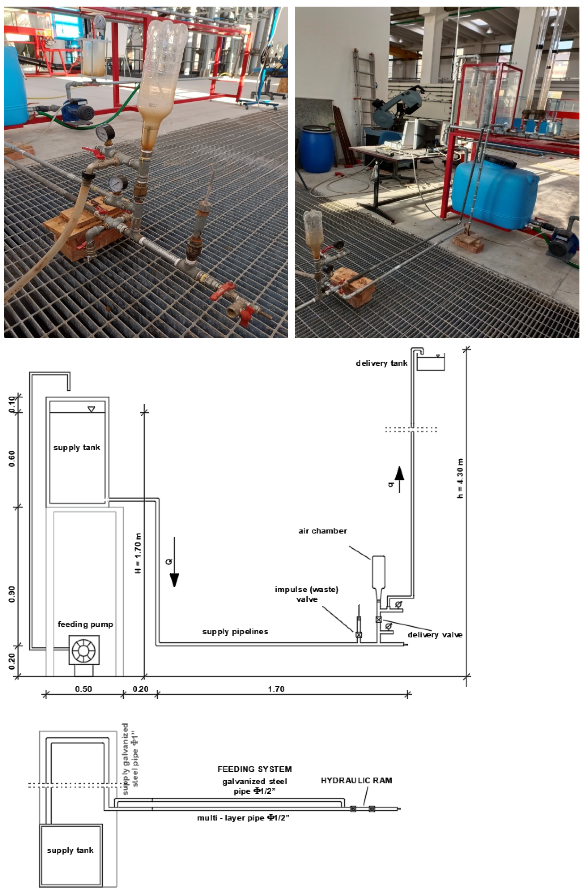
2. Laboratory Experimental Plant

An experimental plant (Figure 3), designed on purpose in order to better study the hydram, was placed at the Laboratory of Environmental and Marine Hydraulics (LIDAM) of the University of Salerno, Italy [37]. A supply tank of 100 L of capacity is fed by a centrifugal pump, model Lowara CEA70/5/A (flow rate range: 30–80 L/min, hydraulic head range: 28.8–20.2 m). The pump is provided with an inverter to adjust the flow rate at the supply tank, with the aim of reaching a steady-state condition with a constant free surface level H = 1.70 m over a time window of some cyclic periods. The supply or drive pipes, upstream of the hydraulic ram, consist of two lines of different materials, a first one made of galvanized steel with nominal diameter DN_gs = 12.7 mm (½ inches), thickness t_gs = 1.3 mm and length L_gs = 3.00 m, and the second one made of multiple layers with nominal diameter DN_ml = 12.7 mm (½ inches), thickness t_ml = 1.0 mm and length L_ml = 2.40 m. These can operate simultaneously or one at a time. In the following, only the galvanized steel pipe is taken into account.

To experimentally detect the rapid pressure variation in the experimental setup described above, sampling high-speed pressure transducers and sampling modules up to 1 kHz were employed. The adopted system of acquisition comprises the following devices:

• Two hydraulic pressure transmitters, model Trafag NAH 8253^®, pressure range 0–2.5 bar (overpressure 5 bar), pressure accuracy 0.15%, sampling rate 1 kHz. Of Wheatstone bridge type, they relate the induced deformation undergone by a membrane to a potential difference proportional to the exerted pressure;
• Two shielded electrical plugs m 12 × 1,5-pole for the electrical connection of the transducers;
• Data acquisition (DAQ) hardware consisting of the National Instruments (NI) cDAQ-9174^® hub, hosting the sampling modules NI 9218^® and NI 9220^®;
• A digital camera, model AOS AOS Q-PRI with a sampling rate of 1 kHz, provided with a 3mp sensor.

Each ram cycle begins with the waste valve fully opened. When the hydrodynamic pressure force acting on the lower side of the impulse valve (Figure 4) wins its weight, the valve starts to rise at an increasing speed and finally closes, depending on its course (Figure 3), yielding a quick increase in pressure locally (onset of the water hammer). The generated positive overpressure now acts against the delivery valve, opening it and inducing a flow of water into the air chamber, which in turn pushes water into the delivery pipe, featuring a maximum elevation h = 4.30 m, up to a delivery tank at a higher elevation. The air chamber prevents the occurrence of shock pressure waves in the delivery pipe, as well as improving the overall pumping efficiency by allowing a more constant flow at the delivery tank. Then, the momentum of the water flowing into the drive pipe decreases to the point that the flow reverses, closing the delivery valve.

Meanwhile, a reflected negative pressure wave is generated at the supply tank when the previous positive impact at its base travels over the drive pipe, causing the lowering of the piston and allowing the process to start again.

3. Numerical Analysis

3.1. CFD

Computational Fluid Dynamics (CFD) is a branch of Fluid Mechanics aimed at simulating the dynamic behaviour of fluids in complex physical problems through the numerical elaboration of sophisticated mathematical models that describe the temporal evolution of the fluid through its fundamental fluid-dynamic parameters: speed, pressure, temperature and density.

The support of numerical modelling is particularly useful, and CFD is an extremely advantageous tool in the design phase, since it allows for analysing different initial configurations in a relatively simple way, both in terms of geometric configurations and boundary conditions, in order to evaluate the responses of the components under consideration in operating conditions close to physical reality and to eliminate, at least in the initial phases, the realization of numerous prototypes when it is necessary to make predictions by analysing a large number of case studies. This virtual simulation is able to provide answers that are consistent with reality, with times and costs significantly reduced compared to the time required for the execution of physical testing. Another great advantage of CFD is independence with respect to the scale factor, which allows for the elimination of visualization problems of fluid dynamic parameters in the simulation of real prototypes. The weaknesses of CFD models are the considerable computational effort required in terms of high calculation times and the need for an optimal degree of expertise by the researcher in the use of the programs. Moreover, the need to numerically integrate equations with a certain degree of complexity and to repeat the calculations on a considerable number of cells is not rare, nor are problems of convergence and stability of the solution, and these are generally resolved by scrupulously defining the calculation grid and correctly setting the boundary conditions.

With reference to the case study at hand, the conceived geometry for the simulation of the dynamic behaviour of the waste valve is simple but at the same time effective. The particular shape of the valve, which depends on the specific vendor, is formulated here in strict terms as a rectangular region whose horizontal dimension is greater than the valve’s free outlet, to allow for complete closure once it has fully risen. The simulations carried out here help in understanding the pressure regime and peak values as the water hammer phenomenon takes place (see Figure 2). In particular, high pressures of the order of hundreds to thousands of kPa can be judged as potentially dangerous for the mechanical system, in terms of integrity or sealing, with the aim of avoiding leakage during operation.

CFD is used mainly to numerically solve the Navier–Stokes equations. Once the geometry of the problem to be simulated has been defined, the volume of fluid involved is divided into a large number of elementary cells that make up the calculation grid.

3.2. CFD Modelling of the Waste Valve

In this work, the behaviour of the waste valve was simulated using the academic version of the software of fluid dynamics computation, ANSYS Fluent^® r14.5 v2012 [38].

In order to carry out the analysis of the discharge valve behaviour, and in particular to simulate the movement of the piston inside it, the overset mesh technique has been used to simplify and speed up the simulations of moving elements within the fluid domain. This technique, in fact, is particularly useful in cases in which a relative movement between components is expected. Compared to remeshing, which involves a regeneration of the cells constituting the mesh of the fluid domain to allow for the movement of the element within it, the overset mesh technique ensures greater control of the characteristics of the domain grid, as individual cells do not have to deform to adapt. The overset mesh allows, therefore, for an optimization of the quality of the cells in reference to the dynamic grids, representing a remarkable advantage from the point of view of the computational cost, both in terms of calculation time and specifications required to perform the simulation.

The following steps were followed to model the simulation of the waste valve’s behaviour:

• Definition of geometry;
• Definition of mesh;
• Setup;
• Solutions and results.

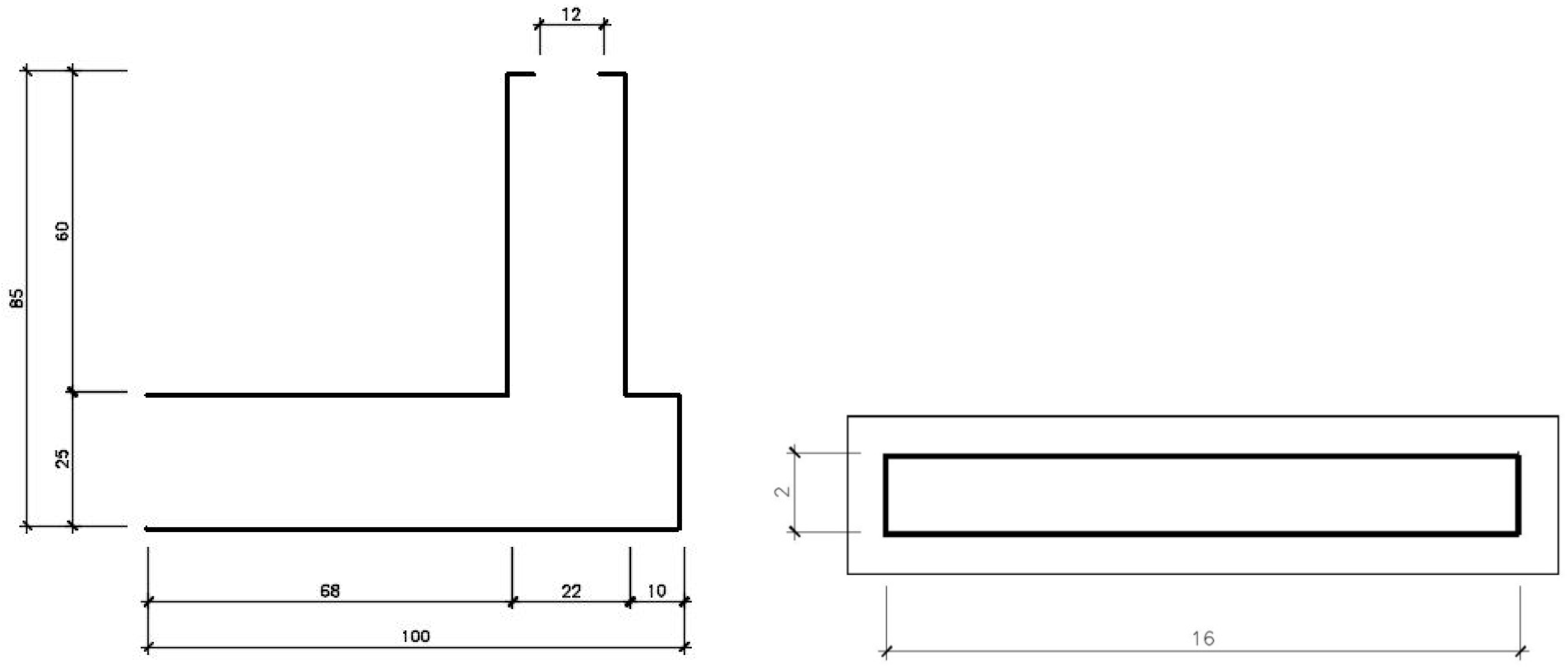
3.3. Geometry Definition

To simulate the behaviour of the waste valve, a simplified geometry is considered, using a two-dimensional representation of the valve and schematizing the piston inside it as a rectangle of size 2 × 16 mm. The overset mesh technique is adopted for the definition of the two geometries and related meshes: one relative to the domain of the fluid within which the movement takes place, i.e., the pump body (Figure 5), and the other representing the moving organ, i.e., the piston inside it (for computational simplicity, represented by a rectangle).

3.4. Definition of the Mesh

An ideal compromise between the accuracy and quality of the fluid dynamic simulation and the necessary cost of computation was sought. The definitions of the two meshes related to the fluid domain and the piston valve were made using a tool on the Workbench platform^® of the ANSYS package.

In order to further improve the mesh quality, additional functions have been added to the two basic configurations, in particular selecting the option to automatically adapt the mesh to the domain (Automatic Method) and to precisely define the mesh organization by selecting quadrilateral cells as predominant (Face Meshing). After a sensitivity analysis, square cells were generated with a side equal to 0.1 mm to ensure proper discretization of the problem.

3.5. ANSYS Fluent Settings for Simulations

The transient (Navier–Stokes) ruling equations are next provided:

$$\overrightarrow{\nabla }·\overrightarrow{\mathbf{v}}=\overrightarrow{\mathbf{0}}$$

(1)

$$\mathsf{\rho }(\frac{\partial }{\partial \mathrm{t}}+\overrightarrow{\mathbf{v}} \overrightarrow{\nabla })\overrightarrow{\mathbf{v}}=-\overrightarrow{\nabla }\mathrm{p}+\overrightarrow{\nabla }·\mathbf{\tau }+\mathsf{\rho }\overrightarrow{\mathbf{g}}$$

(2)

where τ is the stress tensor, $\overrightarrow{\nabla }$ is the nabla operator, $\overrightarrow{\mathbf{v}}$ is the velocity field, $\overrightarrow{\mathbf{g}}$ is the gravity acceleration, p is the pressure, and “·” is the symbol of the scalar product. The standard k-ε (standard wall functions) for turbulence modelling were selected for the calculations. The adopted turbulence model, based on the transport equations for kinetic turbulent energy (k) and the dissipation rate (ε), has been successfully used by many researchers for related CFD problems with moving boundaries (e.g., [24,39]). In particular, the kinetic energy of turbulence k and its dissipation rate ε are obtained from the following transport equations:

$$\frac{\delta }{\delta t}\left(\rho \epsilon \right)+\frac{\delta }{\delta x_i}\left(\rho \epsilon u_i\right)=\frac{\delta }{\delta x_j}\left[\left(\mu +\frac{{\mu }_t}{{\sigma }_{\epsilon }}\right)\frac{{\delta }_{ϵ}}{\delta x_j}\right]+C_{1\epsilon }\frac{\epsilon }{k}\left(G_k+C_{3\epsilon }{G}_b\right)-C_{2\epsilon \rho }\frac{{\epsilon }^2}{k}+S_{\epsilon }$$

(3)

$$\frac{\delta }{\delta t}\left(\rho k\right)+\frac{\delta }{\delta x_i}\left(\rho k{u}_i\right)=\frac{\delta }{\delta x_j}\left[\left(\mu +\frac{{\mu }_t}{{\sigma }_k}\right)\frac{{\delta }_k}{\delta x_j}\right]+G_k+G_b-\rho ϵ-Y_M+S_k$$

(4)

where:

• $G_k$ represents the kinetic energy generation of turbulence due to average speed gradients;
• $G_b$ is the kinetic energy generation of turbulence due to buoyancy;
• $Y_M$ represents the contribution of the fluctuating expansion of compressible turbulence to the overall dissipation rate;
• $C_{1\epsilon }$ = 1.44, $C_{2\epsilon }$ = 1.92 and $C_{3\epsilon }$ = −0.33 are the model constants;
• ${\sigma }_k$ = 1 and ${\sigma }_{\epsilon }$ = 1.3 are the Prandtl turbulence parameters for k and ε, respectively;
• $S_k$ and $S_{\epsilon }$ are user-defined source terms, not included here.

In this case, only the equations of continuity and momentum have been solved as the fluid isothermal. The fluid was set as compressible.

The following boundary conditions were considered: velocity inlet was applied to the fluid inlet (V ≠ 0), wall condition on the solid surfaces surrounding the pump body (∂V/∂n = 0, with $\overrightarrow{\mathbf{n}}$ being the local normal to the wall boundary), the waste valve and the disc and pressure outlet (p = 0) at the outlet of the valve through which water flows. The adopted convergence criterion requires that the scaled residual defined for the continuity equation decreases to 10⁻⁶, whereas for the velocity components, the criterion is 10⁻³. Calculations were performed setting a time step size of 0.001 s. In this way, it was possible to detect the exact instant when the piston is fully raised and a pressure increase took place. All the simulations were performed on an Intel^® Xeon^® CPU E5-1620 3.60 GHz with 64 GB RAM running Windows OS. Computations required a physical time of the order of some minutes.

The progressive closure of the waste valve has been simulated considering that the piston travels a distance of s_max = 30 mm in 0.080 s with a speed of 0.375 m/s (scenario #1 in Section 4.1). Then, it remains closed for 0.140 s. These values were assigned on the basis of the recording taken from the experimental setup [38].

Figure 6 gives information about the frequency of the discharge valve: the stroke s [mm] is plotted versus time t [s] in the two conditions of: (a) progressive closing time of 0.080 s and (b) complete closing time of 0.140 s.

4. Simulations and Analysis of the Results

4.1. List of Performed Simulations

With the aim of analysing the hydrodynamic effects of the waste valve closure, a set of simulations was carried out considering different effective times of progressive closure and complete closure of the valve. Specifically, the performed simulations are listed as follows:

Scenario #1. CFD simulation of the real conditions as recorded in the laboratory, i.e., with a progressive closing time of the discharge valve of 0.080 s and an effective closing time of 0.140 s before the cycle restarts over again. The piston travels s_max = 30 mm in 0.080 s with a speed of V₁ = 0.375 m/s. Assuming the characteristic length D = 12 mm to be the valve outlet, the Reynolds value is Re₁ = 4500;

Scenario #2. Simulation of the valve considering reduced times of 50%, with a progressive closing time of 0.040 s and effective closing time of 0.070 s. The speed for closure is V₂ = 0.75 m/s, and the Reynolds number is therefore Re₁ = 9000. From a physical point of view, it is possible to obtain a similar behaviour of the waste valve, characterized by a reduction in the progressive closing time, by modifying the geometric characteristics of the valve itself. In particular, its frequency beating is increased, and therefore the number of valve beats per minute is increased, decreasing the weight of the piston or increasing the ratio between the diameter of the pump body on which the valve is positioned and the diameter of the piston.

Scenario #3. Simulation of the valve considering times increased by 50% (progressive closing time of 0.120 s and effective closing time of 0.210 s). The speed for closure is V₃ = 0.25 m/s, and the Reynolds number is therefore Re₁ = 3000. From a physical point of view, it is possible to obtain a similar behaviour of the discharge valve, characterized by an increase in the period of progressive closure by decreasing the frequency of the exhaust valve, and therefore the number of beats per minute of the valve, increasing the weight of the piston or reducing the ratio between the diameter of the pump body on which the valve is positioned and the diameter of the piston.

Scenario #4. Simulation of the valve considering times reduced by 25% (progressive closing time of 0.060 s and effective closing time of 0.105 s). The speed for closure is V₄ = 0.50 m/s, and the Reynolds number is therefore Re₁ = 6000.

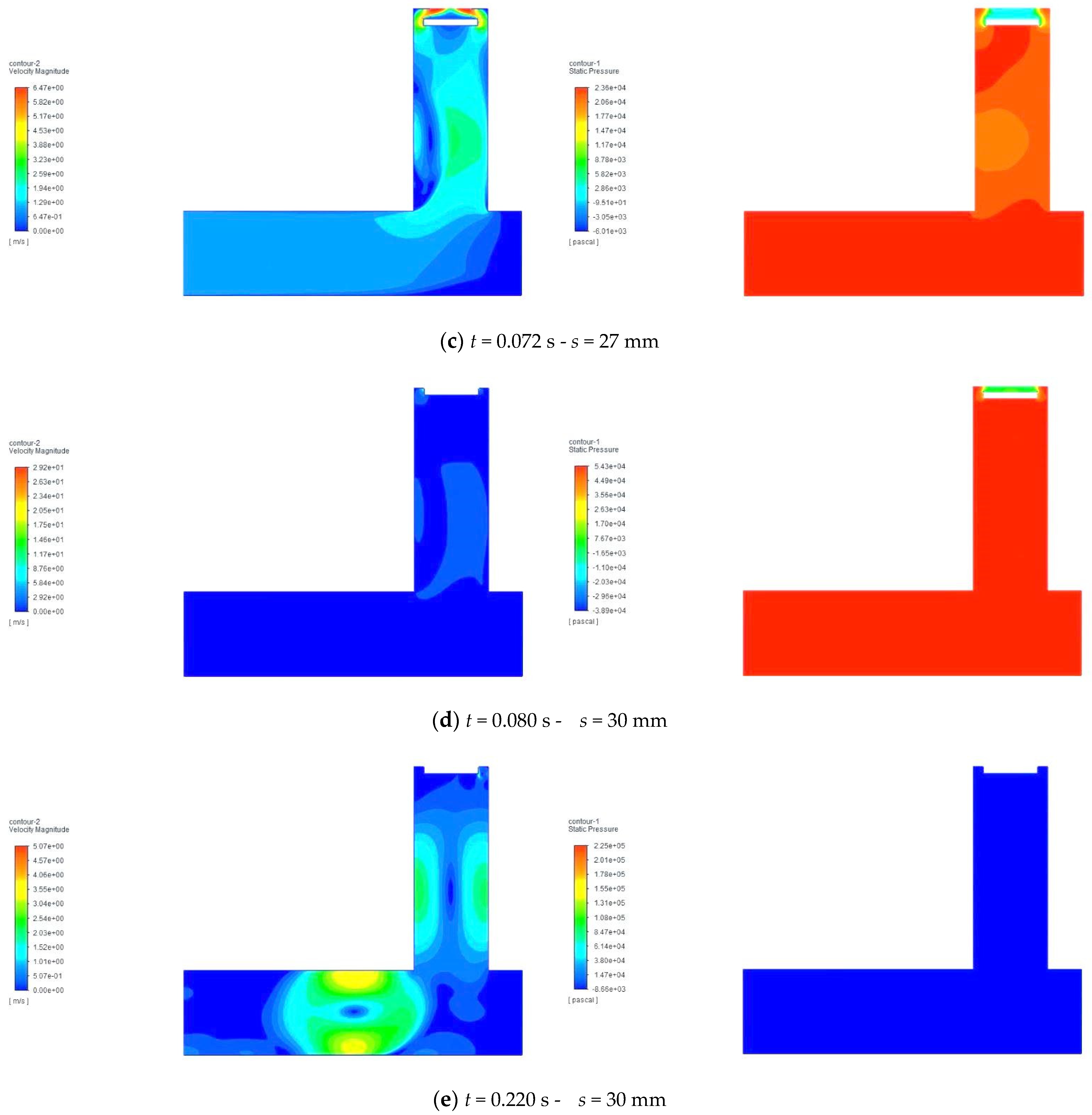
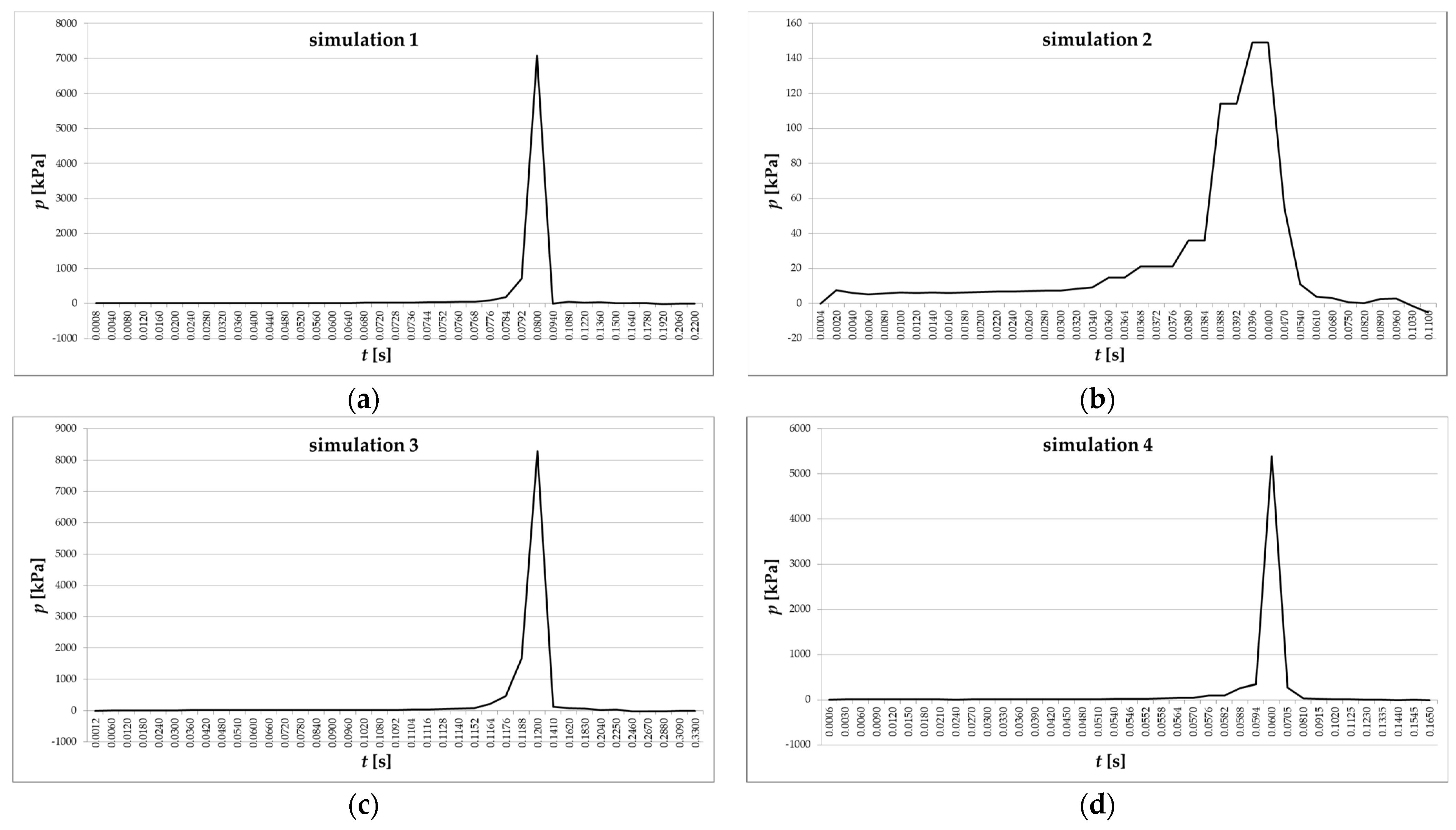
4.2. Velocity and Pressure Analysis for Scenario 1

The simulation results show that the fluid, being able to flow freely through the orifice of the waste valve, progressively increases its velocity during the lifting of the piston (represented in the simulation by a vacuum within the considered fluid domain), passing from an initial value of 1.14 m/s to a value of 29.2 m/s, at which point the sudden closure of the valve occurs. In the instants following the complete lifting of the piston, the water column inside the waste valve stops its stroke, and then it changes its direction of travel by being directed towards the supply line of the system. This speed trend is reflected in the actual operation of the waste valve.

Velocity results for scenario n. 1 are reported in Figure 7 in comparison with a series of frames extrapolated from the simulation, with the trend of the pressures inside the waste valve. Results are given at progressive times t of the simulation, for which the position of the piston is also given (s = 0 corresponds to the half length of the valve and, therefore, s_max = 30 mm).

The results show a progressive increase in the pressure inside the waste valve during the lifting. Coherent with the experimental data, when the valve closes, initially, the recorded pressure variation is very small, and it becomes significant when the complete closure of the waste valve occurs, reaching values on the order of 10⁶ Pa. Initially, the pressure variation is very small, and it becomes significant when the complete closure of the waste valve occurs, reaching values on the order of 10⁵–10⁶ Pa. This sudden change in pressure is consistent with the data collected during the operation of the hydraulic water ram pump at the LIDAM laboratory. The trend of the pressure found during the experiment shows, in fact, a peak at the time of the complete closure of the waste valve. This peak is matched with the values recorded during the simulation, validating the correctness of the numerical model itself.

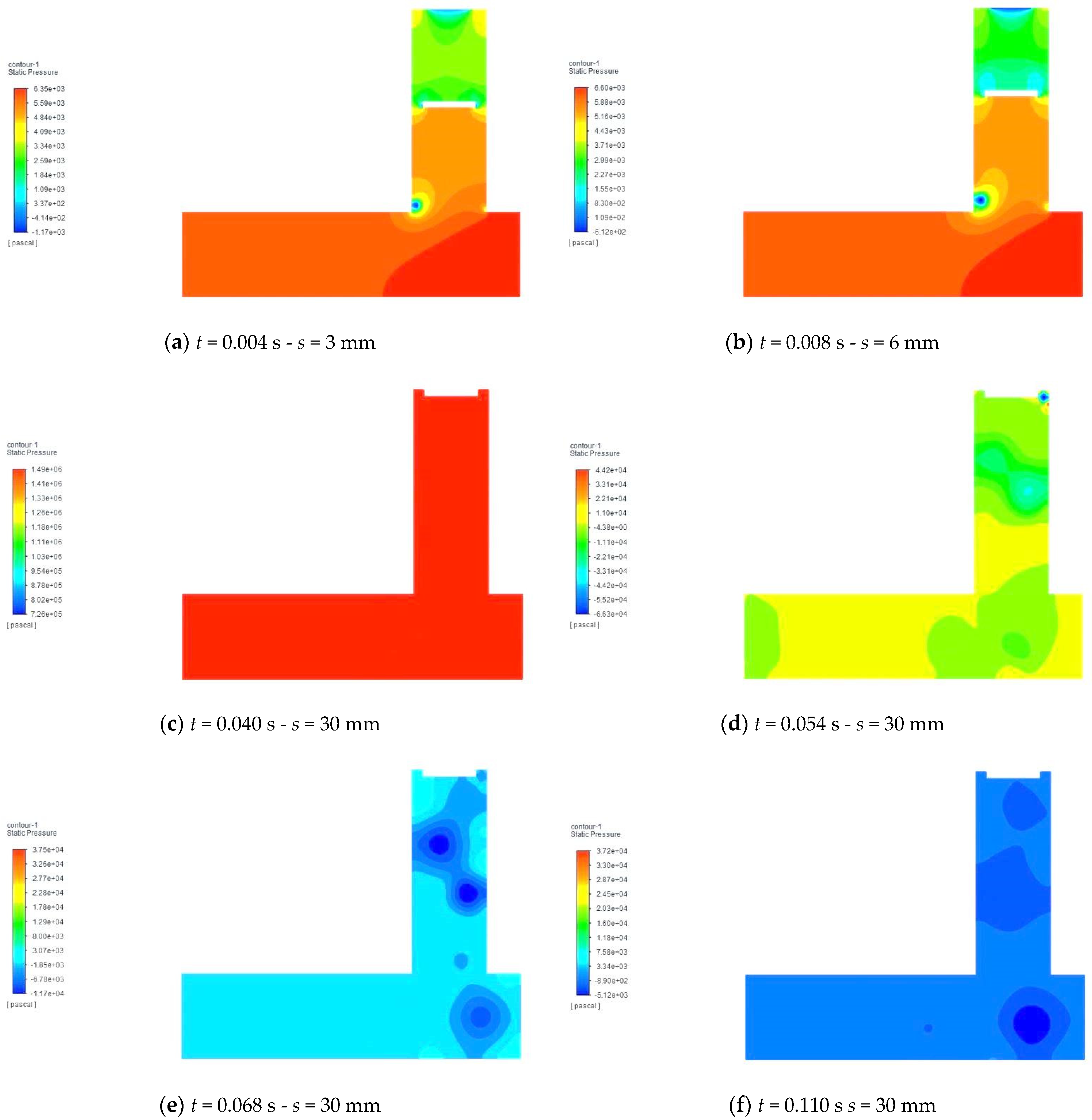
4.3. Pressure Analysis for Scenario 2

Once the behaviour of the valve of the hydram located at the laboratory LIDAM was simulated, the trend in the pressure was evaluated considering different times of progressive closure and total closure of the valve. Initially, the pressure inside the waste valve was assessed considering a progressive closing time of 0.040 s (and then halving the initial simulation period) and an effective closing time in which the piston remains completely raised, equal to 0.070 s.

Figure 8 shows a series of frames extrapolated from the simulation, representing the trend in the pressure inside the waste valve.

4.4. Pressure Analysis: Simulation 3

In addition, the pressure inside the waste valve has been assessed considering a progressive closing time of 0.120 s (therefore doubled compared to the initial case) and an effective closing time in which the piston remains fully raised, equal to 0.210 s.

Figure 9 reports a series of frames extrapolated from the simulation, representing the trend in the pressure inside the waste valve.

4.5. Pressure Analysis: Simulation 4

Finally, the behaviour of the waste valve has been simulated considering a period of progressive closure equal to 0.060 s and a period of effective closure (piston completely raised: s = 30 mm) equal to 0.105 s.

A series of frames extrapolated from the simulation, representing the trend of the pressure inside the waste valve, is reported in Figure 10.

4.6. Comprehensive Analysis of the Results for All Scenarios

Figure 11 shows the time history of the pressure inside the waste valve at the piston lift for the four scenarios (velocity change from the initial value of 1.14 m/s to a value of 29.2 m/s).

The diagram of the second simulation (Figure 11b) shows that by halving the time of progressive closing and effective closing, the pressure inside the waste valve reaches a peak on the order of 10⁶ Pa, which is therefore a value of the same order of magnitude as the initial case. From the physical point of view, it is possible to obtain a similar behaviour of the waste valve, characterized by a reduction in the period of progressive closure, by modifying the geometric characteristics of the valve itself. In particular, this aim is achieved by increasing its frequency and therefore the number of beats per minute of the valve, decreasing the weight of the piston or increasing the ratio between the diameter of the piston and the diameter of the pump body.

The time history of the third simulation (Figure 11c) shows that by increasing the time of progressive closing and of effective closing by 50%, the pressure inside the valve of unloading reaches a corresponding peak on the order of 10⁷ Pa (precisely recording a value of 8.29 × 10⁶ Pa) and therefore a value of the same order of magnitude as the initial case.

The diagram of the fourth simulation (Figure 11d) demonstrates that by reducing the time of progressive closing and of effective closing by 25%, the pressure inside the valve of discharge reaches a corresponding peak of values on the order of 10⁶ Pa (precisely recording a value of 5.39 × 10⁶ Pa) and therefore a value of the same order of magnitude as the initial case, albeit slightly lower.

The obtained pressure peaks are always in the range (∆p J_min, ∆p J_max), with the following pressure surges related to velocity variations obtained from the Joukowsky Equation (see the summary in

Table 1. Expected minimum and maximum pressure variation from the Joukowsky equation.

Scenario	smax (m)	tclosing (s)	Vpiston (m/s)	Vmax_outlet (m/s)	Δp_Jmin (Pa)	Δp_Jmax (Pa)
1	0.03	0.08	0.375	29.20	5.25 × 105	4.09 × 107
2	0.03	0.04	0.75	58.40	1.05 × 106	8.18 × 107
3	0.03	0.12	0.25	38.93	3.50 × 105	5.45 × 107
4	0.03	0.06	0.5	51.91	7.00 × 105	7.27 × 107

for the corresponding values):

∆p J_min = ρ c ∆V_min = ρ c V_piston

(5)

∆p J_max = ρ c ∆V_max = ρ c V_outlet

(6)

where ∆p is the magnitude of the pressure surge caused by the velocity change, ΔV is the velocity change causing the surge, ρ is the fluid density, and c is the wave speed.

From the physical point of view, it is possible to obtain a similar behaviour of the waste valve, characterized by a reduction in the period of progressive closure, by modifying the geometric characteristics of the valve itself. In particular, its frequency is increased, and therefore the number of beats per minute of the valve is increased, decreasing the weight of the piston or increasing the ratio between the diameter of the piston and the diameter of the pump body.

5. Conclusions

In this work, the hydraulic behaviour of a hydraulic ram pump was tested with laboratory experiments and simulations by means of CFD; specifically, the behaviour of the waste valve of the hydram was investigated, whose geometric configuration and operating modes significantly influence the efficiency of the hydram itself.

The results show that an increase in the weight of the waste valve, and in particular of the piston inside it, or a reduction in the ratio between the diameter of the piston and the one of the pump body, implies, under the same boundary conditions, an increase in the acceleration phase of the cycle, the phase during which the water escaping to the outside reaches the critical speed that determines the snap closure of the valve and therefore, consequently, the development of a higher peak pressure inside the system. However, once the critical “maximum” weight of the waste valve has been exceeded, the water, while accelerating progressively, fails to reach the speed necessary to produce a click of the valve, and the automatic operation of the pump stops.

On the other hand, a reduction in the weight of the waste valve, or an increase in the ratio between the diameter of the piston and the diameter of the pump body, involves an increase in the number of beats per minute and a decrease in the volume of water expelled to refusal and therefore a decrease in the acceleration phase of the cycle. At the same time, however, this involves a minor increase in the peak pressure upon closing the waste valve, with the consequent reduction in the water transmitted to the delivery level.

Once the critical minimum value of the drain valve is exceeded, the automatic operation of the valve stops.

The numerical model created turns out to be a valid tool in the design phase of the system, allowing for a reduction in the number of prototypes necessary to identify the ideal configuration of the waste valve, which, under the same boundary conditions, ensures the best performance.

References

1. Clark, J. Hydraulic Rams: Their Principles and Construction; Batsford: London, UK, 1900. [Google Scholar]
2. Anderson, E.W. Hydraulic Rams. Proc. Inst. Mech. Eng. 1922, 102, 337–355. [Google Scholar] [CrossRef]
3. Iversen, H.W. An analysis of the hydraulic ram. J. Fluid Eng. 1975, 97, 191–196. [Google Scholar] [CrossRef]
4. Young, B.W. Generic design of ram pumps. Proc. Inst. Mech. Eng. Part A J. Power Energy 1998, 212, 117–124. [Google Scholar] [CrossRef]
5. Young, B.W. Simplified analysis and design of the hydraulic ram pump. Proc. Inst. Mech. Eng. Part A J. Power Energy 1996, 210, 295–303. [Google Scholar] [CrossRef]
6. Krol, J. The Automatic Hydraulic Ram. Proc. Inst. Mech. Eng. 1951, 165, 53–73. [Google Scholar] [CrossRef]
7. O’brien, M.P.; Gosline, J.E. The Hydraulic Ram; University of California Publications in Engineering: Berkeley, CA, USA, 1933. [Google Scholar]
8. Basfeld, M.; Müller, E. The hydraulic ram. Forsch. Ingenieurwesen 1984, 50, 141–147. [Google Scholar] [CrossRef]
9. Calvert, N.G. Drive Pipe of a Hydraulic Ram. In The Engineer; Harmsworth Press: London, UK, 1958. [Google Scholar]
10. Schiller, E.J.; Kahangire, P. Analysis and computerized model of the automatic hydraulic ram pump. Can. J. Civ. Eng. 1984, 11, 743–750. [Google Scholar] [CrossRef]
11. Mathewson, L. The rebirth of the hydraulic ram pump. Waterlines 1993, 12, 10–14. [Google Scholar] [CrossRef]
12. Najm, H.N.; Azoury, P.H.; Piasecki, M. Hydraulic ram analysis: A new look at an old problem. Proc. Inst. Mech. Eng. Part A J. Power Energy 1999, 213, 127–141. [Google Scholar] [CrossRef]
13. Verspuy, C.; Tijsseling, A.S. Hydraulic ram analysis. J. Hydraul. Res. 1993, 31, 267–278. [Google Scholar] [CrossRef]
14. Young, B.W. Design of hydraulic ram pump systems. Proc. Inst. Mech. Eng. Part A J. Power Energy 1995, 209, 313–322. [Google Scholar] [CrossRef]
15. Othman, M.; Halimee, N.F.H.A.; Sobri, M.N.M.; Suif, Z.; Ahmad, N. Hydraulic Ram Pump: A practical solution for green energy. In Sustainable Development of Water and Environment; Springer International Publishing: Berlin/Heidelberg, Germany, 2020. [Google Scholar] [CrossRef]
16. Li, J.; Yang, K.; Guo, X.; Huang, W.; Shi, C.; Guo, Y.; Wang, T.; Fu, H.; Pan, J. Mathematical model of hydraulic ram pump system. Proc. Inst. Mech. Eng. Part A J. Power Energy 2022, 236, 1097–1108. [Google Scholar] [CrossRef]
17. Filipan, V.; Virag, Z.; Bergant, A. Mathematical modelling of a hydraulic ram pump system. J. Mech. Eng. 2003, 4, 137–149. [Google Scholar]
18. Pathak, A.; Deo, A.; Khune, S.; Mehroliya, S.; Pawar, M.M. Design of hydraulic ram pump. Int. J. Innov. Res. Sci. Technol. 2016, 2, 290–293. [Google Scholar]
19. Sharma, A.M.; Banerjee, D.K.; Pidugu, S.B. Effect of flapper valve on the performance of a hydraulic ram pump. In Proceedings of the ASME 2022 International Mechanical Engineering Congress and Exposition, Columbus, OH, USA, 30 October–3 November 2022. [Google Scholar] [CrossRef]
20. Sharma, A.M.; Jackson, J.H.; Centeno, P.J.; Pidugu, S.B. Effect of source tank configuration on the performance of a hydraulic ram pump. In Proceedings of the ASME 2021 International Mechanical Engineering Congress and Exposition, Online, 1–5 November 2021. [Google Scholar] [CrossRef]
21. Suarda, M.; Ghurri, A.; Sucipta, M.; Kusuma, I.G.W.K. Investigation on characterization of waste valve to optimize the hydraulic ram pump performance. In Proceedings of the International Conference on Thermal Science and Technology (ICTST) 2017, Bali, Indonesia, 17–19 November 2017; Volume 020023. [Google Scholar] [CrossRef]
22. Suarda, M.; Sucipta, M.; Dwijana, I.G.K. Investigation on flow pattern in a hydraulic ram pump at various design and setting of its waste valve. In Proceedings of the IOP Conference Series: Materials Science and Engineering, Bali, Indonesia, 24–25 October 2018; Volume 539, p. 012008. [Google Scholar] [CrossRef]
23. Sucipta, M.; Suarda, M. Investigation and analysis on the performance of hydraulic ram pump at various design its snifter valve. In Proceedings of the IOP Conference Series: Materials Science and Engineering, Bali, Indonesia, 24–25 October 2018; Volume 539, p. 012007. [Google Scholar] [CrossRef]
24. Guo, X.; Li, J.; Yang, K.; Fu, H.; Wang, T.; Guo, Y.; Xia, Q.; Huang, W. Optimal design and performance analysis of hydraulic ram pump system. Proc. Inst. Mech. Eng. Part A J. Power Energy 2018, 232, 841–855. [Google Scholar] [CrossRef]
25. Asvapoositkul, W.; Juruta, J.; Tabtimhin, N.; Limpongsa, Y. Determination of hydraulic ram pump performance: Experimental results. Adv. Civ. Eng. 2019, 2019, 9702183. [Google Scholar] [CrossRef]
26. Fatihhi Januddi, F.S.; Huzni, M.M.; Effendy, M.S.; Bakri, A.; Zulhaimi, M.; Zuhaila, I. Development and testing of hydraulic ram pump (Hydram): Experiments and simulations. In Proceedings of the IOP Conference Series: Materials Science and Engineering 2018, International Fundamentum Science Symposium 2018, Terengganu, Malaysia, 25–26 June 2018; Volume 440, p. 012032. [Google Scholar] [CrossRef]
27. Manohar, K.; Adeyanju, A.A.; Vialva, K. Predicting the output of a hydraulic ram pump. Curr. J. Appl. Sci. Technol. 2019, 38, 1–7. [Google Scholar] [CrossRef]
28. Harith, M.N.; Bakar, R.A.; Ramasamy, D.; Quanjin, M. A significant effect on flow analysis & simulation study of improve design hydraulic pump. In Proceedings of the IOP Conference Series: Materials Science and Engineering 2017, 4th International Conference on Mechanical Engineering Research (ICMER2017), Swiss Garden Beach Resort, Kuantan, Pahang, Malaysia, 1–2 August 2017; Volume 257, p. 012076. [Google Scholar] [CrossRef]
29. Asvapoositkul, W.; Nimitpaitoon, T.; Rattanasuwan, S.; Manakitsirisuthi, P. The use of hydraulic ram pump for increasing pump head-technical feasibility. Eng. Rep. 2021, 3, e12314. [Google Scholar] [CrossRef]
30. Fatahi-Alkouhi, R.; Lashkar-Ara, B.; Keramat, A. On the measurement of ram-pump power by changing in water hammer pressure wave energy. Ain Shams Eng. J. 2019, 10, 681–693. [Google Scholar] [CrossRef]
31. Yussupov, Z.; Yakovlev, A.; Sarkynov, Y.; Zulpykharov, B.; Nietalieva, A. Results of the study of the hydraulic ram technology of water lifting from watercourses. Int. J. Eng. Sci. 2022, 177, 103713. [Google Scholar] [CrossRef]
32. Zeidan, M.; Ostfeld, A. Hydraulic ram pump integration into water distribution systems for energy recovery application. Water 2022, 14, 21. [Google Scholar] [CrossRef]
33. Pawlick, M.; Vaughn, D.; Plumblee, J. Determining Hydraulic Ram Pump Feasibility. J. Humanit. Eng. 2022. [Google Scholar] [CrossRef]
34. Celerinos, P.J.S.; Sanchez-Companion, K.D. Determination of critical delivery head for hydraulic ram pump. Mindanao J. Sci. Technol. 2022, 20, 1–29. [Google Scholar]
35. Widiarta, I.P.; Suarda, M.; Sukadana, I.G.K.; Sucipta, M.; Suantini, N.M.; Suweden, I.N. Study on the waste valve’s stroke to water hammer pressure and flow patterns in a hydraulic ram pump. In Proceedings of the 2nd International Conference on Design, Energy, Materials and Manufacture 2021 (ICDEMM 2021), AIP Conference Proceedings, Pekanbaru, Indonesia, 4 August 2021; AIP Publishing: Melville, NY, USA, 2023; Volume 2568, p. 030014. [Google Scholar] [CrossRef]
36. Handa, C.C.; Valvi, V.; Sahare, M.; Ingole, P.; Samarth, T.; Kumbhare, S.; Raut, A. Development of Hydraulic Ram Pump for Agriculture Uses and Approach A Review. Int. J. Res. Appl. Sci. Eng. Technol. (IJRA) 2023, 11. Available online: www.ijraset.com (accessed on 15 July 2023). [CrossRef]
37. Viccione, G.; Immediata, N.; Cava, R.; Piantedosi, M. A preliminary laboratory investigation of a hydraulic ram pump. In Proceedings of the EWaS3 2018, 3rd EWaS International Conference on “Insights on the Water-Energy-Food Nexus”, Lefkada Island, Greece, 27–30 June 2018; Volume 2, p. 687. [Google Scholar] [CrossRef]
38. ANSYS, Inc. ANSYS Fluent 14.5, Tutorial Guide; ANSYS, Inc.: Canonsburg, PA, USA, 2012. [Google Scholar]
39. Bergamo, U.; Viccione, G.; Coppola, S.; Landi, A.; Meda, A.; Gualtieri, C. Analysis of anaerobic digester mixing: Comparison of long shafted paddle mixing vs. gas mixing. Water Sci. Technol. 2020, 81, 1406–1419. [Google Scholar] [CrossRef]
Figure 1. Sketch of the hydraulic ram pump plant.
Sustainability 15 13104 g001
Figure 2. Water hammer generation. A steady pipe flow, featuring a certain velocity (wider arrow) and pressure (large distance among fluid particles, qualitatively) is suddenly interrupted by a quick closure of the tap, generating a pressure increase nearby (small distance among fluid particles) and low to zero velocity.
Sustainability 15 13104 g002
Figure 3. Experimental setup up of the hydraulic ram pump plant. H is the hydraulic head of the feeding source, h is the hydraulic head of the delivery tank, Q is the drive pipe flow, q is the pumped delivery flow capacity. Waste valve closing times are adopted as input in numerical simulations.
Sustainability 15 13104 g003
Figure 4. Waste valve geometry—section view.
Sustainability 15 13104 g004
Figure 5. Whole Fluid domain and piston geometry.
Sustainability 15 13104 g005
Figure 6. Waste valve time displacement (dotted blue line) from optic laboratory measurements (s is the piston stroke, t is time)—Average values are then extracted (in between dashed grey lines): progressive closing time: 0.080 s; complete closing time: 0.140 s.
Sustainability 15 13104 g006
Figure 7. Simulated velocities and pressures fields at selected time frames for scenario n.1.
Sustainability 15 13104 g007aSustainability 15 13104 g007b
Figure 8. Pressure trends at selected time frames for scenario n.2.
Sustainability 15 13104 g008
Figure 9. Pressure trends at selected frames for scenario n.3.
Sustainability 15 13104 g009
Figure 10. Pressure trends at selected frames for scenario n.4.
Sustainability 15 13104 g010aSustainability 15 13104 g010b
Figure 11. Pressure time trends for scenario 1, 2, 3 and 4, respectively (ad).
Sustainability 15 13104 g011