Article

Prediction of Aircraft Wake Vortices under Various Crosswind Velocities Based on Convolutional Neural Networks

1
School of Air Traffic Management, Civil Aviation Flight University of China, Guanghan 618307, China
2
Institute Office, Civil Aviation Flight University of China, Guanghan 618307, China
*
Author to whom correspondence should be addressed.
Sustainability 2023, 15(18), 13383; https://doi.org/10.3390/su151813383
Submission received: 28 July 2023 / Revised: 31 August 2023 / Accepted: 5 September 2023 / Published: 7 September 2023
(This article belongs to the Special Issue Application of Big Data in Sustainable Transportation)

Abstract

:
In order to overcome the time-consuming computational drawback of using computational fluid dynamics (CFD) for the numerical simulation of aircraft wake vortex evolution under different crosswind velocities, this paper proposes a wake vortex prediction model based on a convolutional neural network (CNN) algorithm. The study focuses on the B737-800 aircraft, and employs CFD numerical simulations to obtain the evolutionary characteristics of wake vortex parameters under crosswind velocities ranging from 0 to 7 m/s. The wake vortex velocity and Q-criterion vorticity values are collected and partitioned into mutually exclusive training and testing datasets. A CNN model is constructed, and the training dataset is used to tune hyperparameters to minimize loss and achieve accurate predictions. After saving the trained model, the desired crosswind velocity value is input to obtain the predicted wake vortex velocity and Q-criterion vorticity values. The results indicate that the convolutional neural network model exhibits an average absolute percentage error of 1.5%, which is 2.3% lower than that of the fully connected neural network model. This suggests that convolutional neural networks can enhance the accuracy of wake vortex predictions, as demonstrated in this study. Compared to traditional CFD methods, the proposed model reduces the computation time by approximately 40 times, effectively improving computational efficiency and offering valuable insight for studies involving numerous numerical simulations, such as analyzing the safety separation between aircraft wake vortices during paired approach procedures.

1. Introduction

A wake vortex is defined as a pair of counter-rotating strong turbulent flows generated at the wingtips during aircraft flight, and it is one of the primary factors affecting aviation safety and efficiency. Currently, research on aircraft wake vortex characteristics, detection, and evolution trends has become a forefront scientific issue in the field of civil aviation air traffic control [1]. During the takeoff and landing phases, aircraft operating on the same runway are required to maintain a minimum longitudinal safety separation, known as wake safety separation, due to the constraints imposed by wake vortices [2]. The main factor determining wake safety separation is the strength of the wake vortex, and meteorological parameters (such as crosswind velocity, atmospheric turbulence dissipation rate, atmospheric stability, etc.) are among the important factors affecting the strength of aircraft wake vortices [3]. Among them, crosswind perturbation on wake vortices is particularly complex, especially during the approach phase, where crosswinds are frequently encountered. With the continuous development of the economy and society, the new runway operation mode is gradually being promoted. The implementation of the paired approach (PA) procedure, which involves simultaneous coordinated approaches of two aircraft on closely spaced parallel runways (CSPRs), has proven effective in alleviating air congestion and enhancing airport operational efficiency [4]. However, during the implementation of this procedure, the wake safety separation between the two aircraft is extremely susceptible to the influence of crosswinds. When the trailing aircraft in the pair mistakenly enters the wake turbulence of the preceding aircraft, it may experience turbulence, rolling, or even engine shutdown, which jeopardizes flight safety [5]. Therefore, it becomes particularly important to determine the impact of wake turbulence generated by the leading aircraft on the following aircraft. Obtaining wake data from the leading aircraft under varying crosswind velocities to determine wake separation poses a challenging problem.
Currently, research methods for wake vortex evolution mainly include laboratory wind tunnel and water tunnel experiments, field radar sensor observations, and computational fluid dynamics simulations [6]. Breitsamter [7] conducted wind tunnel experiments to investigate the variations in wake flow field, focusing on the turbulence intensity, temporal scales, and instability from the near field to the expanded near field during aircraft wake evolution. Bao Feng et al. [8] conducted water tunnel experiments and studied the effects of wake vortex system interactions during aircraft takeoff and landing using particle image velocimetry (PIV) techniques. Babie et al. [9] investigated the influence of a four-vortex model on wake vortex evolution through wind tunnel experiments, revealing that the four-vortex model can induce wake instability and accelerate wake dissipation. Hallock and Holzäpfel [10] presented two methods for collecting aircraft wake vortex-related data: one using pulse laser radar experiments, and the other involving computational fluid dynamics (CFD) simulations of wake vortex evolution. Liu et al. [11] studied the influence of crosswinds on wake vortex evolution using the pulsed coherent Doppler lidar (PCDL) with the range height indicator (RHI) scanning mode. By analyzing the radial velocity and spectral width characteristics, they located the wake vortex core and obtained crosswind information from non-vortex areas within the RHI sector, ultimately obtaining wake vortex trajectories under different crosswind intensities. Dengler et al. [12] investigated aircraft wake vortex trajectories through laser radar wind velocity measurements to estimate the crosswind threshold and provide support for determining safe areas for departing aircraft. Pan et al. [13] conducted wake vortex numerical simulations for the A330 using the SST k-ω turbulence model and compared the results with laser radar observations. They obtained the evolving characteristics of wake vortices under different Brunt-Väisälä frequencies. Robins et al. [14] conducted numerical simulations to investigate the effects of crosswind and ground influence on aircraft wake vortex. The results indicated that the wake vortex generated by larger aircraft near the ground had a severe impact on the flight safety of subsequent smaller aircraft. Proctor et al. [15] used large eddy simulation (LES) to study the influence of crosswinds on aircraft wake vortex evolution, revealing that crosswind shear gradients caused vortices on the left and right sides to descend at different rates, and vortices with the same shear direction as the crosswind tended to persist longer compared to vortices with opposite shear directions. Li et al. [16] investigated the impact of linear and nonlinear environmental crosswinds on a wake vortex through numerical simulations. The results showed that the influence of a uniform linear crosswind and linear vertical shear crosswind on wake vortex strength decreased inversely with the cube of the wake vortex spacing. Zhou et al. [17] established a real-time wake simulation model to study the distribution characteristics of wake states under different crosswind conditions. They demonstrated that crosswind velocities in the range of 1–3 m/s posed the greatest danger, and provided theoretical basis for avoiding wake influence during aircraft flight. Wei et al. [18] employed the Reynolds-averaged Navier–Stokes (RANS) method with the RKE turbulence model, and utilized UDF compilation techniques to apply four different crosswind velocities (0 m/s, 1 m/s, 4 m/s, and 7 m/s) to the A320 wake field, analyzing variations in parameters such as wake sinking, vorticity decay, lateral movement, and wake vortex core velocity under different crosswind conditions. Zhang et al. [19] employed adaptive mesh LES technology to study the evolution and attenuation characteristics of ARJ21 aircraft wake vortices under various crosswind conditions. The numerical simulation results demonstrated that the evolution of vortices upstream and downstream of the aircraft was asymmetric, with the downstream vortices decaying at a faster rate, and the wake vortex dissipation velocity increasing with higher crosswind velocities. He et al. [20] established an aircraft wake vortex model for paired approach procedures, and conducted CFD numerical simulations to analyze the wake characteristics. Based on the simulation results, they proposed an optimization method for longitudinal safety separation of paired aircraft wake vortices. Ma et al. [21] conducted an analysis of the evolution characteristics of paired aircraft wake under crosswind conditions of 1 m/s, 3 m/s, and 5 m/s using the CFD method, and obtained the wake safety separation of the paired aircraft.
As evident from the preceding discussion, numerous scholars have delved deeply into the field of wake vortex research. The aforementioned methods allow for the acquisition of data with high reliability and accuracy, as well as detailed information regarding wake vortex evolution. However, it is worth noting that the implementation of these methods invariably demands a significant amount of time. In comparison to wind tunnel experiments, water tunnel experiments, and radar sensor observations, the CFD method requires only computer resources and software, which significantly reduces equipment costs and computational expenses. Nonetheless, simulating wake vortex evolution using CFD necessitates partitioning the aircraft model into millions or even tens of millions of grid cells to ensure simulation accuracy, resulting in computation times ranging from hours to days. Additionally, when studying wake vortex evolution under different crosswind velocities, recalculations are necessary with each change in the crosswind parameter, further prolonging the overall research duration.
In addressing the aforementioned issue of lengthy computation times, numerous scholars have begun to employ neural networks for flow field predictions. Carpenter et al. [22] introduced a single-hidden-layer neural network for predicting missile aerodynamic parameters. Balla et al. [23] proposed a multi-output neural network for predicting the aerodynamic coefficients of two-dimensional and three-dimensional wings, demonstrating superior performance compared to their intrinsic proper orthogonal decomposition (POD) counterparts. Wang et al. [24] presented a depth-based learning model, which effectively reduces computational costs while obtaining more accurate flow field characteristics. Silva et al. [25] introduced a CFD-based non-steady-state aerodynamic reduced-order model (ROM) that minimizes recognition errors. Tracey et al. [26] trained neural networks on data generated by the Spalart–Allmaras model, replicating flow conditions under different circumstances. Ling et al. [27] proposed a deep neural network method based on the RANS approach for simulating the Reynolds stress tensor.
From the literature mentioned above, it is evident that employing neural networks for the resolution and prediction of fluid flows has emerged as a novel trend in fluid dynamics forecasting. Trained convolutional neural networks (CNNs), as highlighted in [28], serve to reduce computational costs by taking on a portion of the numerical solving process. Simultaneously, they enable efficient utilization of CFD data, thereby preventing resource wastage. Therefore, in this study, CFD methods were utilized to numerically simulate the evolution characteristics of tail vortices under various crosswind velocities. The simulated wake vortex feature data was employed as the input dataset for a CNN model, which was subsequently trained and its network structure saved. This trained model was then used for wake vortex predictions by inputting desired crosswind velocity values. The feasibility of this method was verified by comparing it with the basic FCNN method in flow field prediction. This method enhances the computational efficiency of wake vortex predictions, optimally utilizes CFD data, and conserves computational resources. It provides a theoretical foundation for the implementation of new operational modes, such as paired approach procedures, which rely heavily on extensive numerical simulations to determine wake separation safety distances.

2. Research Methods

2.1. Convolutional Neural Network Algorithm

The CNN has emerged as a prominent method in deep learning and has found extensive applications in the field of air traffic control in recent years. Typically, a CNN consists of input layers, hidden layers, and output layers, where the hidden layers comprise the convolutional layer, pooling layer, and fully connected layer [29], as illustrated in Figure 1. The one-dimensional convolutional neural network (1DCNN) model exhibits distinct advantages over a simple FCNN in predicting aircraft wake vortex velocities. One-dimensional CNNs leverage parameter sharing and translational invariance when handling sequential data, which aids the model in better comprehending local features and spatial relationships within the input data. One-dimensional CNNs employ convolutional kernels for convolution operations, which can be regarded as features learned by the model, thus enhancing interpretability. However, the 1DCNN is currently unable to predict wake vortex velocities and vortex cloud images under different wind speeds based on the wake vortex velocities and vortex cloud images derived from CFD calculations. Therefore, further research is warranted to explore the application of convolutional neural networks in wake vortex prediction.

2.2. Forecasting Process

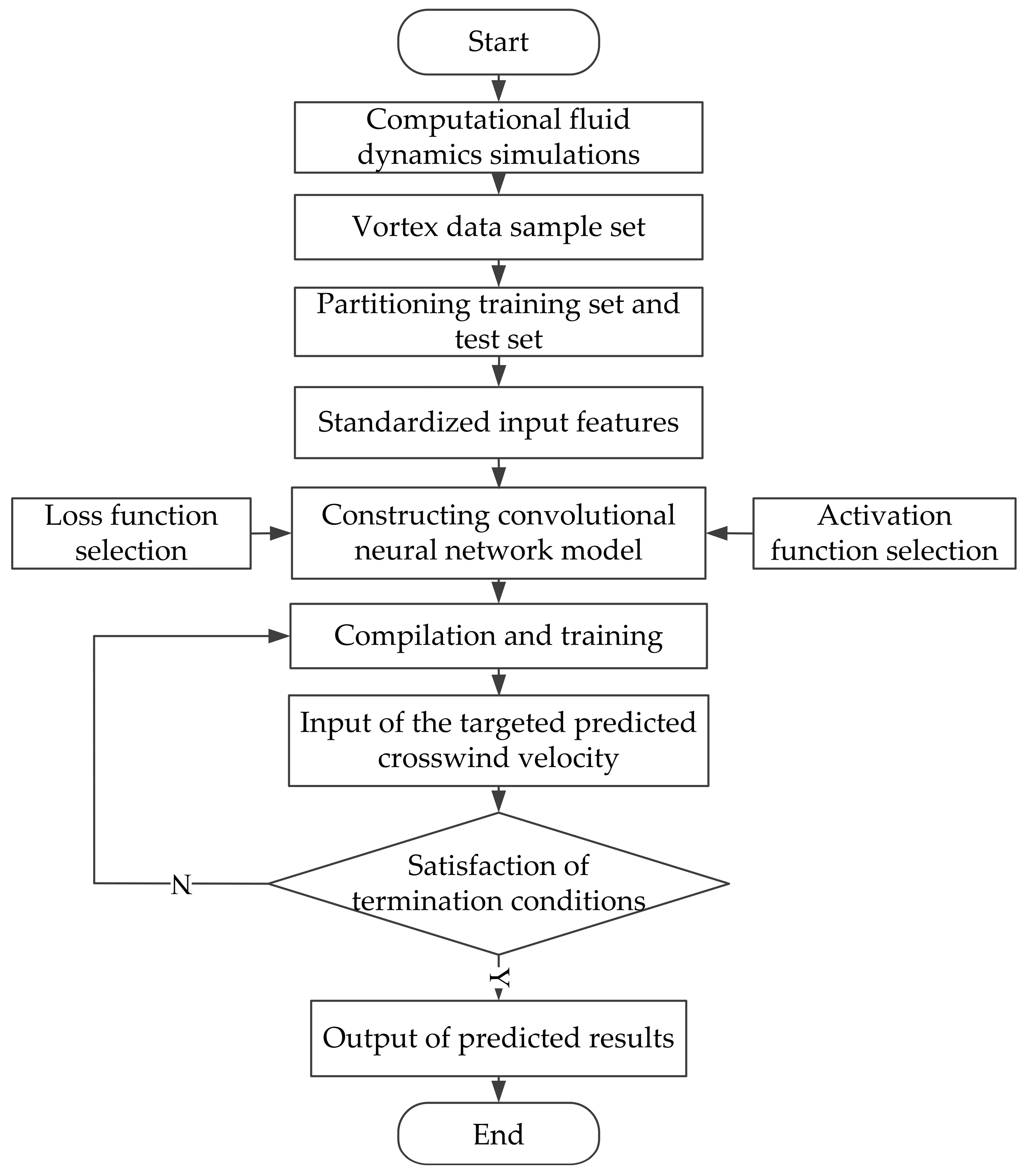
On the basis of the data obtained from CFD simulations, this study employs CNN for the prediction of wake vortices under different crosswind velocities, ultimately establishing a generalized predictive model. The training process is illustrated in Figure 2. The CFD data is divided into mutually exclusive training and testing sets, which serve as input samples for the neural network. The input features are standardized. A CNN is constructed, and the training set samples are fed into the network while adjusting hyperparameters to minimize loss on the training set and achieve accurate predictions from the model. After saving the trained model, the prediction data is fed into the neural network to obtain the predicted wake vortex velocity and Q criterion vorticity values. Subsequently, these predictions are compared with the actual samples to validate the accuracy of the predictive model.

2.3. Acquisition of Data Sample Sets

This study employs a Latin hypercube sampling technique to extract 50 distinct wind velocities ranging from 0 to 7 m/s, ensuring the randomness and uniformity of the training data. CFD simulations are conducted using these selected wind velocities to simulate the wake vortex evolution process and obtain the data sample sets. Each set comprises 1000 data points for both wake vortex velocity and Q-criterion vorticity values, which are randomly divided into an 80% training set and a 20% testing set.

2.3.1. Geometric Model and Grid Partitioning

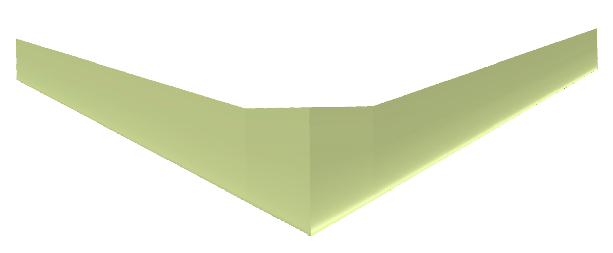
In this study, a simplified B737-800 wing was created using Catia P3 V5R21 software, with a wingspan of 34.31 m, as shown in Figure 3.
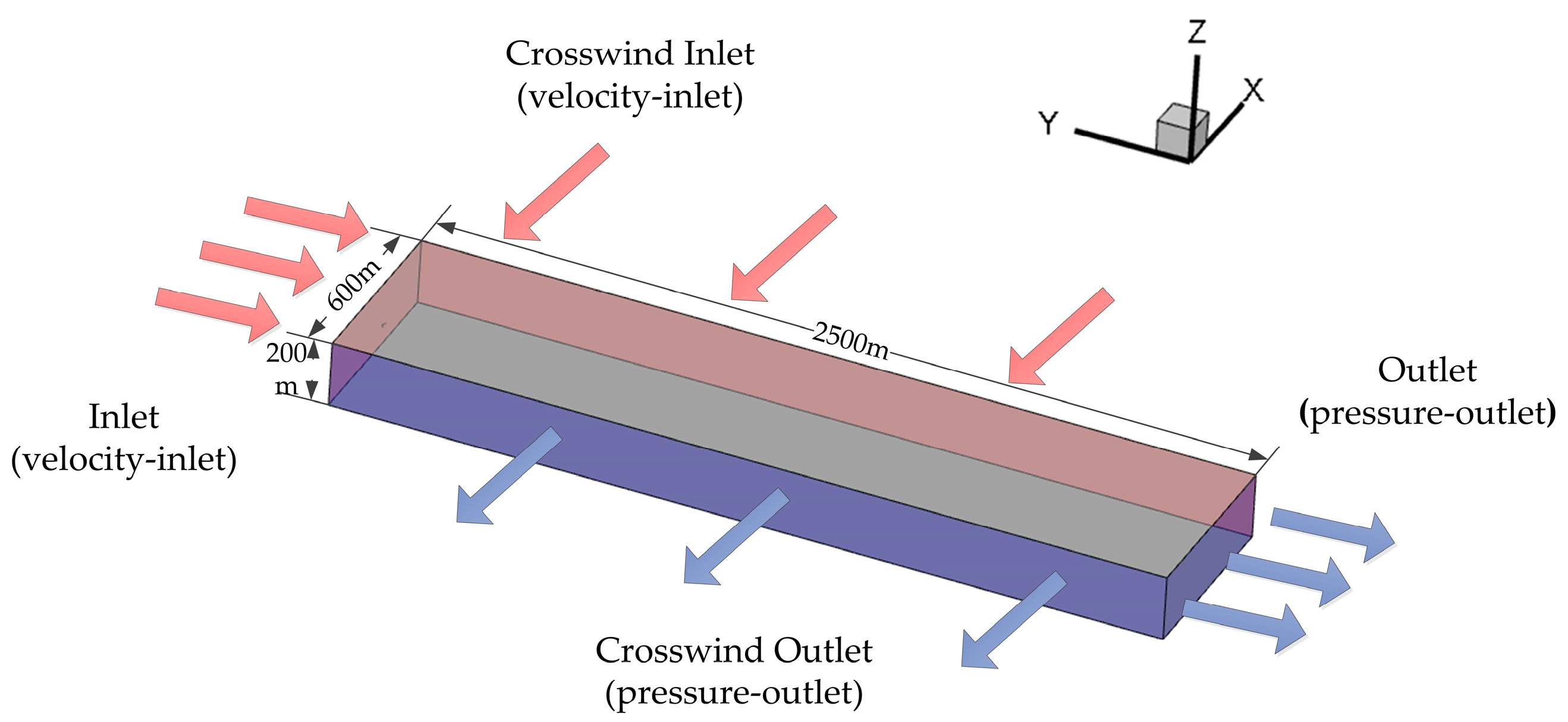
A hexahedral computational domain with dimensions of 2500 m × 600 m × 200 m was established, as depicted in Figure 4. In Figure 4, red arrows represent incoming gas, while blue arrows represent outgoing gas. The model’s coordinate origin was set at the trailing edge of the wing, with the x-axis representing the wingspan direction, the y-axis representing the wing chord direction, and the positive direction of the z-axis indicating the lift direction.
To enhance computational efficiency and improve stability, this study employed a high-precision structured hexahedral mesh. The O-block technique was utilized to refine the grid density around the wing, enhancing the orthogonality of the grid near the wing. The final distribution of the grid in the flow field region and around the wing is illustrated in Figure 5.

2.3.2. Control Equations

In this study, the RANS method was employed to analyze the evolution process of wake vortices, which offers advantages of lower computational time and hardware costs [30]. The fundamental idea of the RANS method is to decompose turbulent flow. The RANS method decomposes the variables satisfying the dynamic instantaneous Navier-Stokes equations into mean and turbulent components. By substituting the velocity components, pressure components, and energy components into the instantaneous continuity and momentum equations, the N–S equations in Cartesian coordinates are derived.
The expressions for the continuity and momentum equations are presented in Equations (1) and (2), respectively.
ρ t + x i ( p u i ) = 0
t ( ρ u i ) + x i ( p u i u j ) = p x i + σ i j x j + x j ( ρ u i u j )
In the equation, ρ represents the atmospheric turbulence density; u i is the mean velocity component in the x i direction; u j is the mean velocity component in the x j direction; p denotes the atmospheric pressure; u i u j is the stress term in the Reynolds-averaged Navier–Stokes equation; and σ i j represents the components of the stress tensor.

2.3.3. Turbulence Model

The SST k-ω turbulence model was selected for this study. The fundamental idea behind this model is to use the k-ω model near the wall, and the k-ε model in the boundary layer edge and free shear layer. As a result, the SST k-ω model combines the advantages of both the k-ω and k-ε models. The transport equations for k and ω in the SST k-ω model are as follows:
t ( ρ k ) + x i ( p k u i ) = p x i [ Γ k k x j ] + G k + S k Y k
t ( ρ ω ) + x i ( p ω u i ) = p x i [ Γ ω ω x j ] + G ω + S ω + D ω Y ω
Γ k = μ + μ t σ k
Γ ω = μ + μ ω σ ω
In the equations: μ represents turbulent viscosity; Γ k and Γ ω are the diffusion rates; G k and G ω denote turbulent kinetic energy; S k and S ω are user-defined terms; Y ω and Y k represent turbulent diffusion production; D ω is the orthogonal divergence term; and σ k and σ ω are the turbulence energy Prandtl coefficients.

2.3.4. Boundary Conditions

The entire computational domain was configured as a hexahedral model, with the inlet boundary set as a velocity inlet, the outlet as a pressure outlet, and the walls as no-slip solid surfaces. Based on the approach and departure scenarios of the B737-800, the temperature was set to 288.15 K, atmospheric pressure to 101, 325 Pa, and the inflow velocity to 72 m/s.

2.4. Correlation Analysis

The linear relationships among the parameters were assessed using the Pearson correlation coefficient method, with the specific calculation formula shown in Equation (7).
r = 1 n 1 i = 1 n ( X i X ¯ s X ) ( Y i Y ¯ s Y )
In the equation: X i X ; Y i Y ; X and Y represent two sequences to be predicted; X ¯ and Y ¯ represent the means of the sequences X and Y to be predicted; and n is the length of the sequences to be predicted.
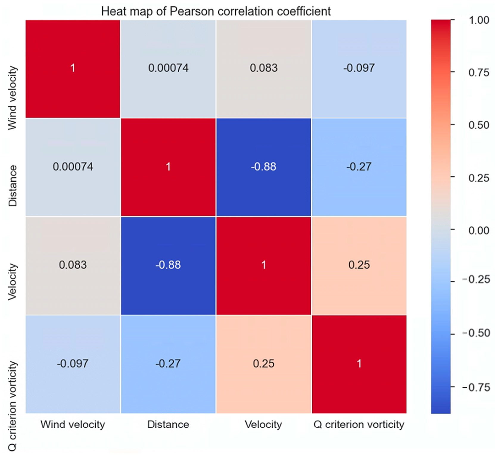
From Figure 6, it is evident that the correlation coefficient between wake vortex velocity and distance is −0.88, while the correlation coefficient between wake vortex Q-criterion vorticity and distance is −0.27. Additionally, the correlation coefficients between crosswind velocity and wake vortex velocity, as well as crosswind velocity and Q-criterion vorticity, are 0.083 and −0.097, respectively. A larger absolute value of the correlation coefficient indicates a stronger correlation between two feature vectors. Comparing the correlation coefficients of distance and crosswind velocity with aircraft wake vortex velocity and Q-criterion vorticity reveals that distance has a significant impact on both variables. However, the impact of crosswind velocity on these variables cannot be overlooked, particularly in the practical operations of aircraft. With the advancement of dynamic and precise wake separation techniques, the influence of crosswind on wake turbulence separation has gained growing attention from professionals in the civil aviation industry.

2.5. Activation Function Selection

The activation functions express the non-linear relationships of data distribution, and the mathematical formulas for the Sigmoid function, Tanh function, ReLU function, and Leaky ReLU function, are shown in Equations (8)–(11) respectively.
s i g m o i d ( x ) = 1 1 + e x
tanh ( x ) = e x e x e x + e x
Re LU ( x ) = max ( 0 , x )
Leaky Re LU ( x ) = max ( 0.01 x , x )  
When the input values are small, the output of the Sigmoid function approaches 0, indicating that the function responds weakly or neglects small input values. As the input values gradually increase, the output of the Sigmoid function increases, representing a stronger response to the input information. The Tanh function can be derived from the evolution of the Sigmoid function, and both functions have similar variance values for numerical terms in forward and backward propagation. The Tanh function has a variance value closer to zero, and the stochastic gradient descent velocity can approach the natural gradient more, leading to faster convergence. The ReLU function is a non-saturating nonlinearity with a non-zero centered characteristic, which possesses sparse representation capability. However, it tends to suffer from the vanishing gradient problem when the input value x is negative. On the other hand, the Leaky ReLU function is an improved algorithm over ReLU, introducing a negative slope for negative values of x instead of directly setting them to zero, thus avoiding the vanishing gradient issue. Therefore, in this study, the Leaky ReLU function is chosen as the activation function for the convolutional layers, as it can better support the training of deep networks, control model complexity, enhance the performance of predicting wake vortex velocity and vorticity, and improve the model’s generalization ability to new samples.

2.6. Loss Function Selection

The loss function is primarily employed to assess the predictive performance of the neural network model, and serves as the optimization target during the model training process. It quantifies the discrepancy between the predicted values and the actual target values of the input samples, where a smaller value of the loss function indicates more accurate predictions. As the flow field prediction problem falls under the category of regression tasks, this study adopts a commonly used loss function for regression problems, namely the mean squared error (MSE) loss function. The specific expression is shown in Equation (12).
M S E ( y i , y i ) = i = 1 n ( y i y i ) 2 n
In the equation, y i represents the true value of the i-th data point in the dataset, and y i represents the predicted value of the i-th data point in the dataset. The variable n represents the total number of predicted data points, and MSE represents the mean squared error, which is the average error of the batch of data.

3. Prediction Result Analysis

3.1. Model Training

We constructed a data processing, model training, and data prediction framework using the Python programming language and the TensorFlow deep learning framework. The input data includes the distance from the wing trailing edge and crosswind velocity, while the output consists of predicted wake vortex velocity and Q-criterion vorticity values. The 1DCNN model comprises a single convolutional layer with 64 filters, a kernel size of 2, and Leaky ReLU activation function. It has one flatten layer and three fully connected layers. The optimizer used is Adam. The FCCN model has two hidden layers with 64 and 32 neurons, respectively, and an output layer with 2 neurons.

3.2. Result Analysis

The evolution of aircraft wake flow can be broadly divided into four regions: the near field, expanded near field, mid/intermediate field, and dissipation field, as shown in Figure 7. The near field is the region where the wake is generated, and the wake height is concentrated in this region. In the expanded near field, the wake undergoes processes of rolling up, merging, and shedding. As the wake progresses into the mid/intermediate field, linear instability occurs. In the dissipation field, strong interactions between left and right vortices occur until dissipation is complete.
The Q criterion is a physical criterion used to describe the vortical structures and evolution in fluid flow, aiming to quantify the presence and strength of vortices in the flow field. This criterion determines the presence of vortices by calculating the velocity gradient tensor of the fluid velocity field, and evaluates the strength of vortices using the eigenvalues of this gradient tensor. The two-dimensional non-dimensional Q criterion in the Oxz plane can be expressed as follows:
Q = 1 2 [ ( u x ) 2 + ( v z ) 2 ] u z v x
where u and v represent the velocity components in the x and z directions, respectively.
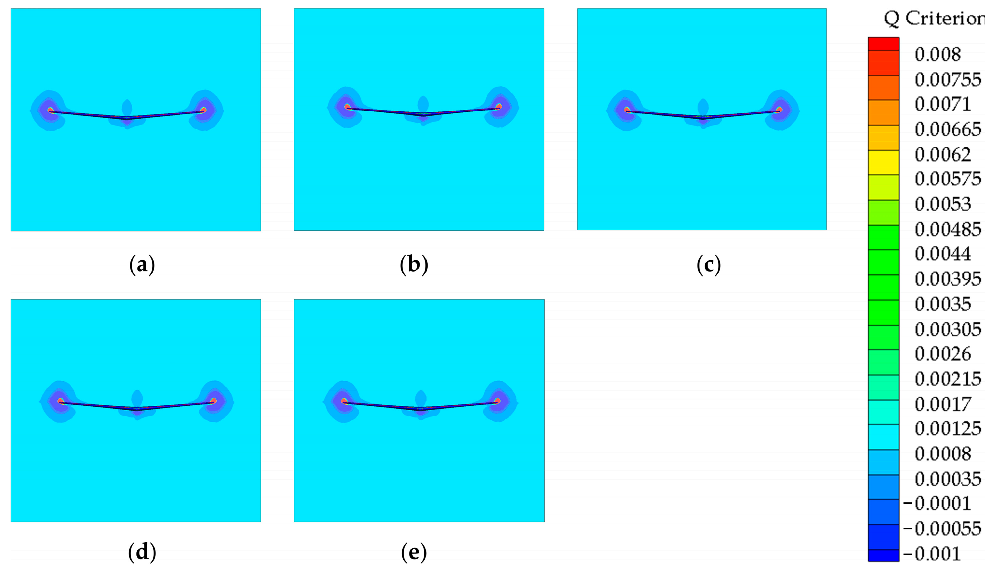
Due to the relatively weaker intensity of the wake in the mid/intermediate field and dissipation field, this study analyzes the Q criterion vorticity values at two positions: Y/b = 0.5, which is at a distance of 0.5 wing spans behind the wing (near-field), and Y/b = 5, which is at a distance of 5 wing spans behind the wing (expanded near-field). As a right crosswind is considered in this study, the right vortex is referred to as the upwind vortex, and the left vortex is referred to as the downwind vortex. In the following context, Y/b = i represents the distance from the wing trailing edge to the i-th wingspan. From Figure 8, it can be observed that as the right crosswind velocity increases, the vortex strength in the wake at Y/b = 0.5 remains relatively unchanged. This is due to the initial formation stage of the wake, which exhibits some degree of symmetry, resulting in a balanced aerodynamic force between the left and right vortices, countering the effect of the crosswind.
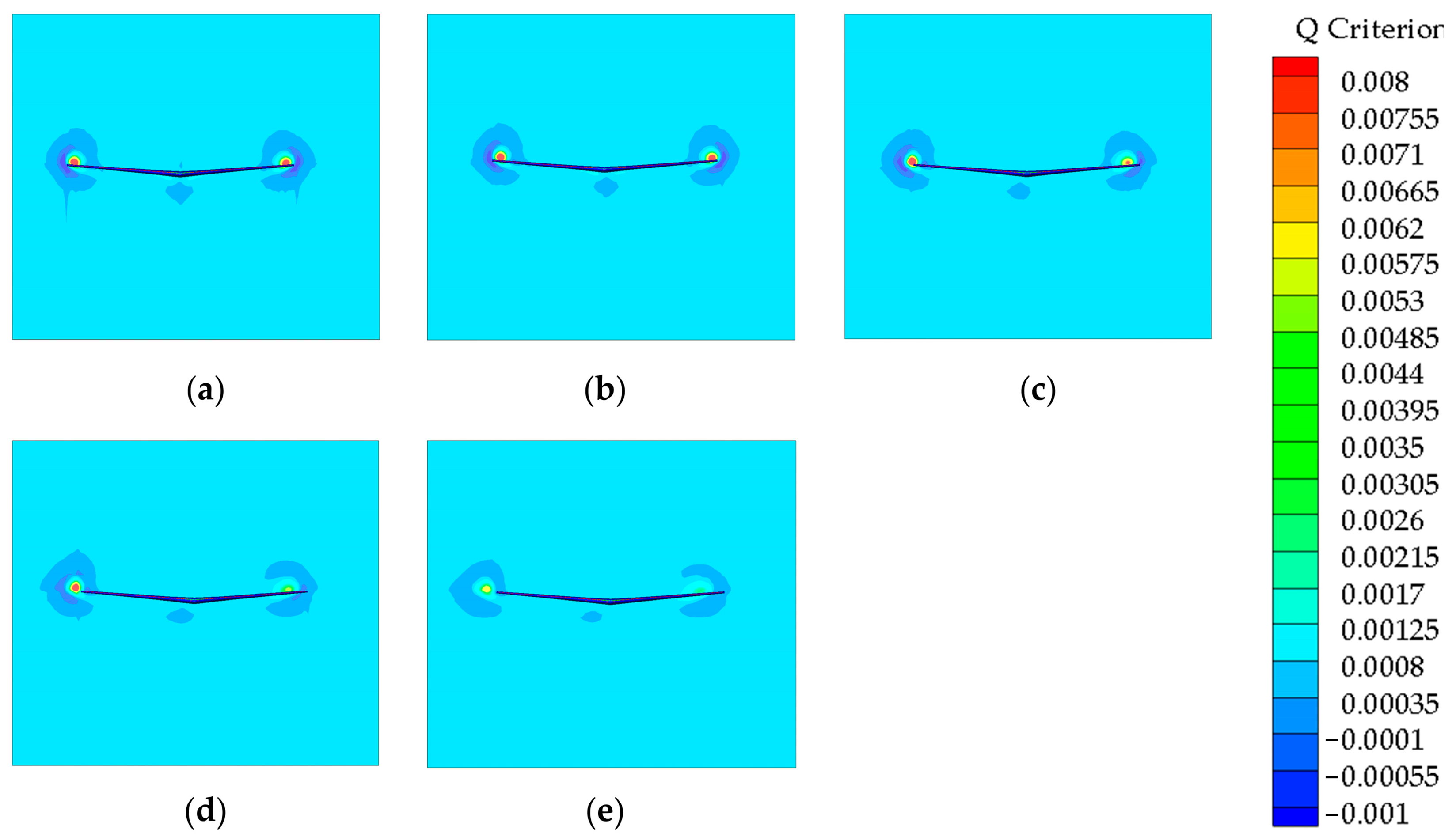
From Figure 9, it can be observed that under the same crosswind velocity conditions, the difference between the vortex structures and the velocity gradient tensor eigenvalues at Y/b = 5 is significantly smaller than at Y/b = 0.5. This indicates that the vortex intensity decreases as it develops from a distance of 0.5 wing spans behind the wing to a distance of 5 wing spans behind the wing. With the continuous increase in crosswind velocity, the vortex intensity at Y/b = 5 shows a clear decreasing trend. When the crosswind velocity is 3 m/s, the left and right vortices exhibit asymmetric behavior, which becomes more pronounced at crosswind velocities of 5 m/s and 7 m/s. This phenomenon indicates that as the crosswind velocity increases, the velocity shear effect on the wake at Y/b = 5 gradually intensifies, leading to a reduction in vortex intensity. The upwind vortex is directly affected by the crosswind, which enhances the turbulence kinetic energy and increases the Q-criterion vorticity values. Additionally, the crosswind reduces the influence of viscous resistance on the airflow, which slows down the decay rate of the wake vortex.
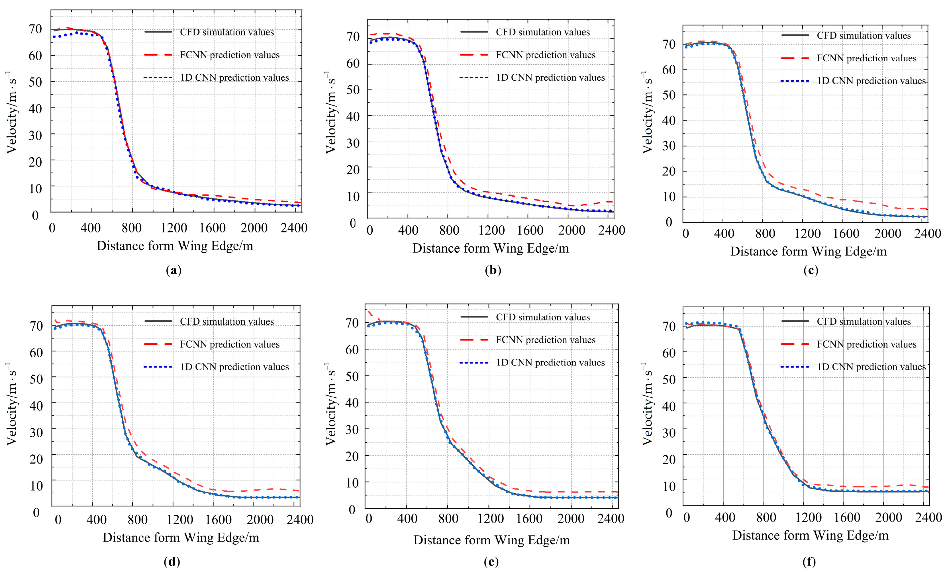
From Figure 10 and Figure 11, it can be observed that for crosswind velocities ranging from 0 to 7 m/s, when 0 m ≤ Y ≤ 600 m, the slope of the wake vortex velocity curve is nearly zero, indicating that the wake vortex is spreading at a stable rate during this phase. For 600 m ≤ Y ≤ 1000 m, the slope of the wake vortex velocity curve is higher, suggesting an acceleration in the dispersion of the wake vortex. Beyond Y > 1000 m, the slope of the wake vortex velocity curve decreases, signifying that the wake vortex has entered a stable dissipation phase. Comparing Figure 10 and Figure 11, it can be noted that for Y ≥ 600 m, increasing crosswind velocity significantly enhances the lateral vortex velocity. This phenomenon occurs because lower crosswind velocities are insufficient to disrupt the integrity of the wake vortex morphology, while higher crosswind velocities induce the separation of the primary vortex body from the wake vortex core, accelerating the dissipation of the wake vortex. Furthermore, the upstream vortex velocities, starting from the point of acceleration and dissipation, are consistently lower than the downstream vortex velocities. This is attributed to the shear effects of the downstream vortex, which induce significant variations in horizontal airflow velocity. This stronger shear effect leads to increased twisting and stretching of the vortex, thereby hastening its dissipation. Based on Figure 9 and Figure 10, it is observed that the disparity between the blue curve and the black curve is smaller across various crosswind speed conditions compared to that of the red curve and the black curve. This implies that the predictive performance of the 1DCNN model outperforms that of the FCNN model.
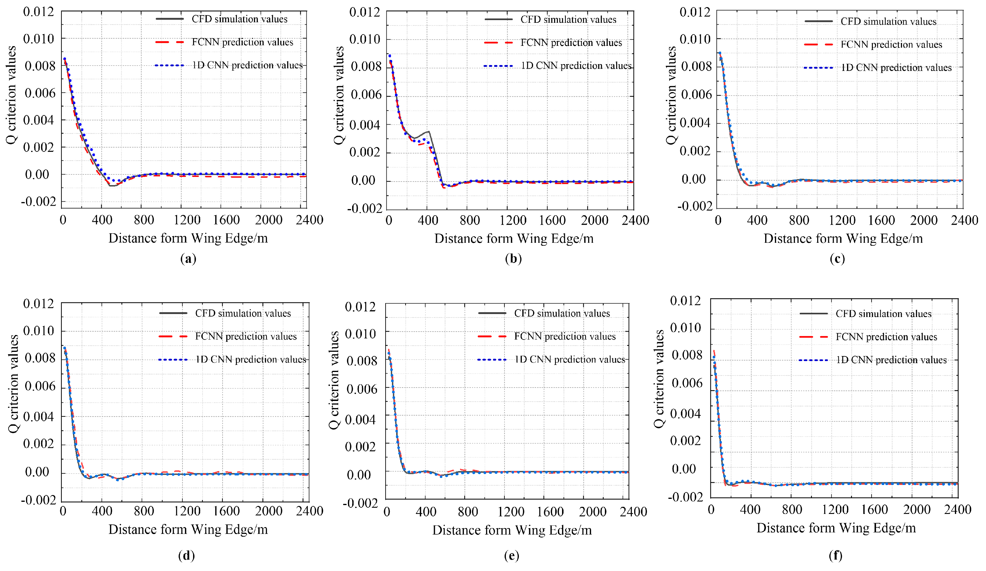
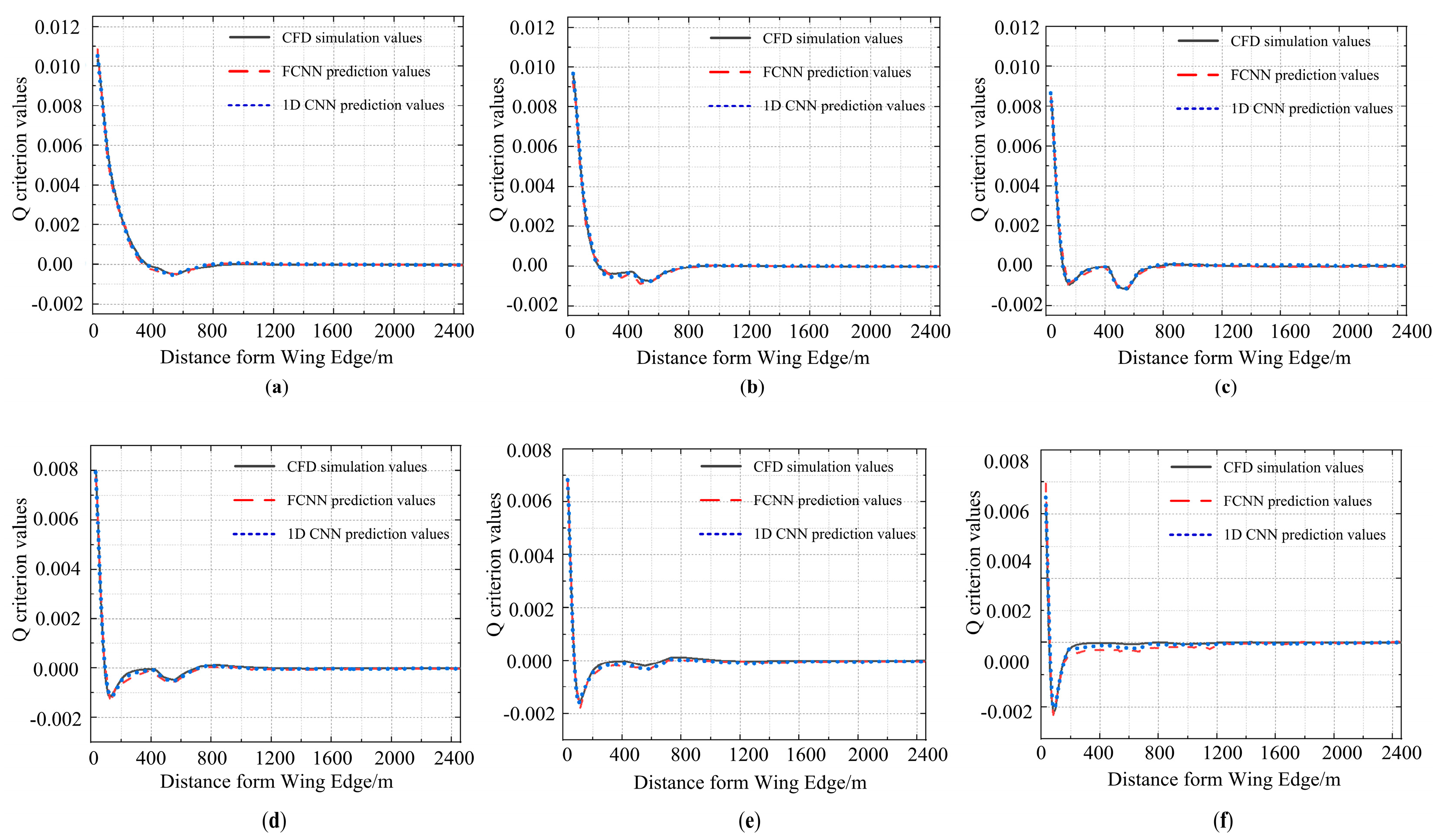
Figure 12 and Figure 13 illustrate the consistent variation trend of the Q criterion for both the left and right vortices under crosswind conditions ranging from 0 to 7 m/s. Within the range of 0 ≤ Y ≤ 500 m, the Q criterion vorticity values for the vortices demonstrate a sharp decrease with a significant slope. Beyond Y ≥ 500 m, the Q criterion vorticity values exhibit a nearly constant slope close to zero. The uneven distribution of Q criterion vorticity values for the vortices is attributed to the additional pressure and velocity gradients induced by the crosswind, causing perturbations in the vortices. The comparative results between the predicted values and actual values across Figure 10, Figure 11, Figure 12 and Figure 13 collectively demonstrate the neural network model’s strong robustness in wake vortex prediction.
Table 1 reveals that the average absolute percentage errors (MAPE) for predicting wake vortex velocity and Q-criterion vorticity under different crosswind conditions through 1DCNN and FCNN are 1.15% and 3.8%, respectively. The 1DCNN model exhibits a 2.3% reduction in MAPE compared to the FCNN model. An R-squared (R2) value of 0.987 for the 1DCNN model indicates excellent fitting capabilities.
The purpose of this study is to establish a rapid model for predicting the characteristics of wake vortex evolution based on a CNN. Therefore, the computational time of the model is an important metric for evaluating its performance. The computational times for predicting wake vortex velocity and intensity using both the CFD method and the CNN algorithm were recorded on a platform with Win10 Professional, an Intel (R) Xeon (R) CPU E5-2620 v4 @ 2.10 GHz processor, and 16GB RAM. During the CFD simulation, the average time for one iteration step in the convergence process of 10,000 steps was 6.63 s, while for the CNN-based wake vortex prediction model, the average time for one iteration step in the convergence process of 10,000 steps was 0.153 s. It is evident that the CNN-based wake vortex prediction model, compared to the traditional CFD method, significantly reduces the computational time after neural network training is completed.

4. Conclusions

In this study, the CNN method was employed to predict the wake vortex velocity and Q criterion values under different crosswind velocities using data obtained from CFD numerical simulations. The conclusions are summarized as follows:
(1)
Utilizing a 1DCNN for the prediction of wake vortex velocity and Q-criterion vorticity under crosswind velocities ranging from 0 to 7 m/s resulted in an average absolute percentage error of 1.5%. This represents a 2.3% reduction in error compared to the FCNN model, highlighting the superior predictive accuracy of this model. Furthermore, this model has improved computational efficiency by approximately 40 times compared to traditional CFD methods.
(2)
Crosswinds have a certain influence on the evolution of wake vortex velocity. Lower crosswinds do not significantly disrupt the wake vortex structure, while higher crosswinds can disrupt the wake vortex structure and accelerate its dissipation. Moreover, under the influence of crosswinds, the velocity of the upwind vortex is generally lower than that of the downwind vortex, starting from the acceleration and dissipation stage.
(3)
Crosswinds also have an impact on the intensity of the wake vortex. Due to the direct interaction of crosswinds with the upwind vortex, the crosswinds increase the turbulence kinetic energy of the airflow and reduce the effect of viscous resistance, resulting in an increase in the intensity of the upwind vortex and a slowdown in the decay rate of the wake vortex.
(4)
This study provides significant insights for the research on paired approach wake separation, and the proposed model effectively reduces the computation time for the wake evolution characteristics of the leading aircraft. This study provides the potential for a more detailed exploration of the wake separation safety distance for paired aircraft under different crosswind velocities.
This study has only considered the influence of crosswind velocity and wake vortex evolution distance on wake vortex velocity and Q-criterion vorticity. Moreover, it has established a 1DCNN for preliminary data prediction. In the future, a more comprehensive approach can be pursued by developing more intricate convolutional neural networks to predict wake vortex characteristics under different crosswind velocities, encompassing aspects such as wake vortex pressure, wake vortex offset distance, wake vortex core separation, and other relevant factors.

Author Contributions

Conceptualization, X.H. and R.Z.; methodology, X.H. and H.G.; software, X.H.; validation, X.H. and R.Z.; formal analysis, H.G. and R.Z.; investigation, C.Y. and J.W.; resources, X.H. and H.G.; data curation, X.H.; writing—original draft preparation, R.Z. and C.Y.; writing—review and editing, X.H. and H.G.; visualization, X.H. and R.Z.; supervision, X.H.; project administration, H.G.; funding acquisition, X.H. All authors have read and agreed to the published version of the manuscript.

Funding

This research was funded by the Civil Aviation Administration of China Security Capability Project: Study on Safety Separation Interval for Aircraft Operations Behind Jet Blast Effects During Takeoff, No. [2022] 186, Research and Innovation Team of Civil Aviation Flight University of China: Flight Efficiency Improvement Research Center, Institution No. CZKY2023156, and Graduate Innovation Project Funding from Civil Aviation Flight University of China: Study on Arrival Runway Capacity Based on Runway Occupancy Time and Wake Turbulence Separation, No. X2023-42.

Institutional Review Board Statement

Not applicable.

Informed Consent Statement

Not applicable.

Data Availability Statement

The datasets generated during and/or analyzed during the current study is available from the corresponding author on reasonable request.

Conflicts of Interest

The authors declare no conflict of interest.

References

  1. Shen, C.; Li, J.B.; Gao, H.; Chen, B.W.; Han, Q.G.; Wang, X.S. Aircraft wake vortex behavior prediction based on data assimilation. J. Radars 2021, 10, 632–645. [Google Scholar] [CrossRef]
  2. Lin, M.D.; Cui, G.X.; Zhang, Z.S.; Xu, C.X.; Huang, W.X. Large eddy simulation on the evolution and the fast-time prediction of aircraft wake vortices. Chin. J. Theor. Appl. Mech. 2017, 49, 1185–1200. [Google Scholar] [CrossRef]
  3. Holzäpfel, F. In Sensitivity analysis of the effects of aircraft and environmental parameters on aircraft wake vortex trajectories and lifetimes. In Proceedings of the 51st AIAA Aerospace Sciences Meeting including the New Horizons Forum and Aerospace Exposition, Grapevine, TX, USA, 7–10 January 2013; p. 363. [Google Scholar] [CrossRef]
  4. Mundra, A.D.; Cooper, W.W.; Smith, A.P.; Audenaerd, L.F.; Lunsford, C.R. In Potential benefits of a paired approach procedure to closely spaced parallel runways in instrument and marginal visual conditions. In Proceedings of the 2008 IEEE/AIAA 27th Digital Avionics Systems Conference, St. Paul, MN, USA, 26–30 October 2008; pp. 3.C.4-1–3.C.4-16. [Google Scholar]
  5. Gerz, T.; Holzäpfel, F.; Bryant, W.; Köpp, F.; Frech, M.; Tafferner, A.; Winckelmans, G. Research towards a wake-vortex advisory system for optimal aircraft spacing. Comptes Rendus Phys. 2005, 6, 501–523. [Google Scholar] [CrossRef]
  6. He, X.; Wang, X.; Zhang, W.W.; Jiang, H. Review of the experiment, modeling and simulation of wing tip wake. Flight Dyn. 2019, 5, 1–6. [Google Scholar] [CrossRef]
  7. Breitsamter, C. Wake vortex characteristics of transport aircraft. Prog. Aerosp. Sci. 2011, 47, 89–134. [Google Scholar] [CrossRef]
  8. Bao, F.; Liu, J.S.; Zhu, R.; Liu, Y. Experimental study on Rayleigh-Ludwieg instability of aircraft wake vortex. Acta Aeronaut. Et Astronaut. Sin. 2015, 36, 2166–2176. [Google Scholar] [CrossRef]
  9. Babie, B.M.; Nelson, R.C. In Wavelength and amplitude measurement of an unstable wake vortex bending mode via helium-bubble visualization. In Proceedings of the 13th International Symposium on Flow Visualization, Nice, France, 1–4 July 2008. [Google Scholar]
  10. Hallock, J.N.; Holzapfel, F. A review of recent wake vortex research for increasing airport capacity. Prog. Aerosp. Sci. 2018, 98, 27–36. [Google Scholar] [CrossRef]
  11. Liu, X.Y.; Zhang, X.Y.; Zhai, X.C.; Zhang, H.W.; Liu, B.Y.; Wu, S.H. Observation of Aircraft Wake Vortex Evolution under Crosswind Conditions by Pulsed Coherent Doppler Lidar. Atmosphere 2021, 12, 49. [Google Scholar] [CrossRef]
  12. Dengler, K.; Holzapfel, F.; Gerz, T.; Wiegele, A.; De Visscher, I.; Winckelmans, G.; Bricteux, L.; Fischer, H.; Konopka, J. Crosswind thresholds supporting wake-vortex-free corridors for departing aircraft. Meteorol. Appl. 2012, 19, 289–301. [Google Scholar] [CrossRef]
  13. Pan, W.J.; Jiang, Y.Q.; Zhang, Y.Q. Simulation Study of the Effect of Atmospheric Stratification on Aircraft Wake Vortex Encounter. Sustainability 2023, 15, 6391. [Google Scholar] [CrossRef]
  14. Robins, R.E.; Delisi, D.P. Potential hazard of aircraft wake vortices in ground effect with crosswind. J. Aircr. 1993, 30, 201–206. [Google Scholar] [CrossRef]
  15. Proctor, F.; Ahmad, N.; Switzer, G. In Crosswind shear gradient affect on wake vortices. In Proceedings of the 3rd AIAA Atmospheric Space Environments Conference, Honolulu, HI, USA, 27–30 June 2011; p. 3038. [Google Scholar] [CrossRef]
  16. Li, D.; Xu, Z.M.; Zhang, K.; Zhang, Z.Y.; Zhou, J.X.; Pan, W.J.; Wang, X. Study on the influence of linear and nonlinear distribution of crosswind on the motion of aircraft wake vortex. Proc. Inst. Mech. Eng. Part G-J. Aerosp. Eng. 2021, 235, 1981–1990. [Google Scholar] [CrossRef]
  17. Zhou, B.; Wang, X.S.; Wang, T.; Liu, J.K. Influence of crosswind velocities on aircraft wake vortex movement. Acta Aeronaut. Et Astronaut. Sin. 2009, 30, 773–779. [Google Scholar]
  18. Wei, Z.Q.; Li, Z.Y.; Liu, W. Research on Aircraft Wake Vortex Strength Dissipation and Vortex Motion under Crosswind Impact. Journal of Air Force Engineering University: Nat. Sci. Ed. 2017, 18, 27–33. [Google Scholar] [CrossRef]
  19. Zhang, J.D.; Zou, Q.H.; Lin, M.D.; Huang, W.X.; Pan, W.J.; Cui, G.X. Numerical simulation on near-field evolution of wake vortices of ARJ21 plane with crosswind. Acta Aeronaut. Et Astronaut. Sin. 2022, 43, 163–175. [Google Scholar]
  20. He, X.; Ma, Y.L.; Yang, H.; Chen, Y.Q. Modeling and Simulation of Wake Safety Interval for Paired Approach Based on CFD. J. Adv. Transp. 2021, 2021, 7891475. [Google Scholar] [CrossRef]
  21. Ma, Y.L. Research of Paired Approach Wake Safety Zone Based On CFD; Civil Aviation Flight University of China: Deyang, China, 2021. [Google Scholar] [CrossRef]
  22. Carpenter, M.; Hartfield, R.; Burkhalter, J. In A comprehensive approach to cataloging missile aerodynamic performance using surrogate modeling techniques and statistical learning. In Proceedings of the 29th AIAA Applied Aerodynamics Conference, Honolulu, HI, USA, 27–30 June 2011; p. 3029. [Google Scholar] [CrossRef]
  23. Balla, K.; Sevilla, R.; Hassan, O.; Morgan, K. An application of neural networks to the prediction of aerodynamic coefficients of aerofoils and wings. Appl. Math. Model. 2021, 96, 456–479. [Google Scholar] [CrossRef]
  24. Wang, Z.; Xiao, D.; Fang, F.; Govindan, R.; Pain, C.C.; Guo, Y. Model identification of reduced order fluid dynamics systems using deep learning. Int. J. Numer. Methods Fluids 2018, 86, 255–268. [Google Scholar] [CrossRef]
  25. Silva, W.A. Simultaneous excitation of multiple-input/multiple-output CFD-based unsteady aerodynamic systems. J. Aircr. 2008, 45, 1267–1274. [Google Scholar] [CrossRef]
  26. Tracey, B.D.; Duraisamy, K.; Alonso, J.J. In A machine learning strategy to assist turbulence model development. In Proceedings of the 53rd AIAA Aerospace Sciences Meeting, Kissimmee, FL, USA, 5–9 January 2015; p. 1287. [Google Scholar] [CrossRef]
  27. Ling, J.; Kurzawski, A.; Templeton, J. Reynolds averaged turbulence modelling using deep neural networks with embedded invariance. J. Fluid Mech. 2016, 807, 155–166. [Google Scholar] [CrossRef]
  28. Le, T.-T.-H.; Kang, H.; Kim, H. Towards Incompressible Laminar Flow Estimation Based on Interpolated Feature Generation and Deep Learning. Sustainability 2022, 14, 11996. [Google Scholar] [CrossRef]
  29. Pan, B.; Yu, H.; Cheng, H.; Du, S.; Cai, S.; Zhao, M.; Du, J.; Xie, F. A CNN–LSTM Machine-Learning Method for Estimating Particulate Organic Carbon from Remote Sensing in Lakes. Sustainability 2023, 15, 13043. [Google Scholar] [CrossRef]
  30. He, X.; Yuan, C.; Gao, H.; Chen, Y.; Zhao, R. Calibration of Turbulent Model Constants Based on Experimental Data Assimilation: Numerical Prediction of Subsonic Jet Flow Characteristics. Sustainability 2023, 15, 10219. [Google Scholar] [CrossRef]
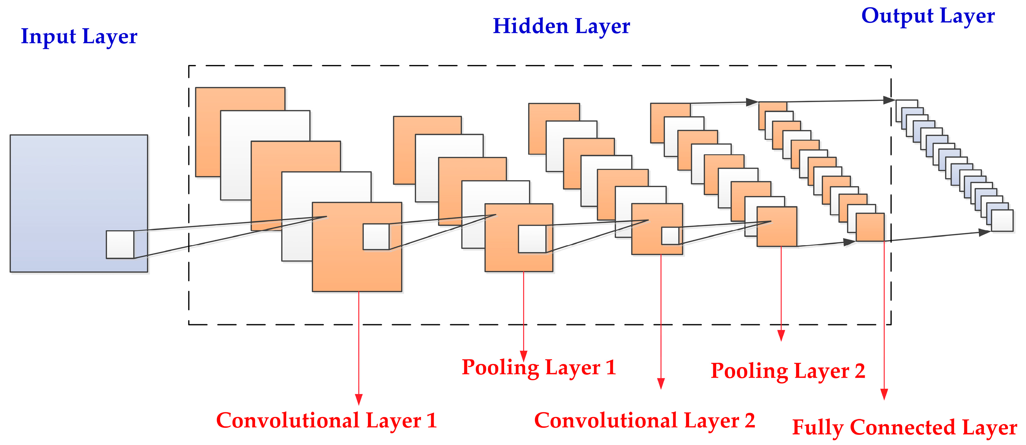
Figure 1. Structure diagram of a convolutional neural network.
Sustainability 15 13383 g001
Figure 2. Convolutional neural network training flow.
Sustainability 15 13383 g002
Figure 3. Geometric model of B737-800 wing.
Sustainability 15 13383 g003
Figure 4. Schematic of the computational domain for flow field simulation.
Sustainability 15 13383 g004
Figure 5. Grid distribution.
Sustainability 15 13383 g005
Figure 6. Pearson correlation coefficient heatmap.
Sustainability 15 13383 g006
Figure 7. Wake flow field division.
Sustainability 15 13383 g007
Figure 8. Q-criterion vorticity field maps at 0.5 wingspan distance behind the wing at different crosswind velocities: (a) 0 m/s; (b) 1 m/s; (c) 3 m/s; (d) 5 m/s; (e) 7 m/s.
Sustainability 15 13383 g008
Figure 9. Q-criterion vorticity field maps at 5 wingspan distance behind the wing at different crosswind velocities: (a) 0 m/s; (b) 1 m/s; (c) 3 m/s; (d) 5 m/s; (e) 7 m/s.
Sustainability 15 13383 g009
Figure 10. Comparison of predicted right vortex velocities to CFD simulation values at different crosswind velocities: (a) 0.2 m/s; (b) 1.6 m/s; (c) 2.8 m/s; (d) 3.8 m/s; (e) 4.7 m/s; (f) 6.3 m/s.
Sustainability 15 13383 g010
Figure 11. Comparison of predicted left vortex velocities to CFD simulation values at different crosswind velocities: (a) 0.2 m/s; (b) 1.6 m/s; (c) 2.8 m/s; (d) 3.8 m/s; (e) 4.7 m/s; (f) 6.3 m/s.
Sustainability 15 13383 g011
Figure 12. Comparison of predicted right vortex Q-criterion vorticity values to CFD simulation values at different crosswind velocities: (a) 0.2 m/s; (b) 1.6 m/s; (c) 2.8 m/s; (d) 3.8 m/s; (e) 4.7 m/s; (f) 6.3 m/s.
Sustainability 15 13383 g012
Figure 13. Comparison of predicted left vortex Q-criterion vorticity values to CFD simulation values at different crosswind velocities: (a) 0.2 m/s; (b) 1.6 m/s; (c) 2.8 m/s; (d) 3.8 m/s; (e) 4.7 m/s; (f) 6.3 m/s.
Sustainability 15 13383 g013
Table 1. Presents the evaluation metrics for prediction accuracy.
Name.Mean Squared
Error (MSE)
Mean Absolute Percentage Error (MAPE%)R-Squared (R2)
1DCNN1.571.5%0.987
FCNN3.353.8%0.984
Disclaimer/Publisher’s Note: The statements, opinions and data contained in all publications are solely those of the individual author(s) and contributor(s) and not of MDPI and/or the editor(s). MDPI and/or the editor(s) disclaim responsibility for any injury to people or property resulting from any ideas, methods, instructions or products referred to in the content.