The Routing Problem for Electric Truck with Partial Nonlinear Charging and Battery Swapping

Abstract

The maritime industry has introduced the concept of “green ports” as a means to achieve sustainable development by reducing carbon emissions. Within ports, trucks play a crucial role in transportation operations. However, there is limited comprehensive research on the electric truck routing problem containing practical constraints such as charging options and charging processes. This study presents a more realistic routing problem for electric trucks, with a specific focus on multiple charging options within green ports. To address this challenge, we formulate a mixed-integer programming model designed to minimize overall operational costs associated with the transportation of trucks over the planning horizon. In order to solve this problem effectively, we devise an Adaptive Large Neighborhood Search (ALNS) algorithm, embedded with several customized operators. Through a series of numerical experiments, the effectiveness of the proposed algorithm is verified. The experimental results provide compelling evidence of the superior performance of the proposed algorithm compared to the original ALNS algorithm. Furthermore, sensitivity analysis is conducted, leading to valuable managerial insights.

1. Introduction

The pressing challenge of escalating greenhouse gas (GHG) emissions and the imperative for sustainable development in the shipping industry call for the construction of green ports. Global GHG emissions, primarily ${\mathrm{CO}}_2$ (25%), rose from 52.82 billion tons in 2016 to 54.59 billion in 2021, with an increase of 3.4% [1]. Recognized as the principal driver of climate change [1], GHG emissions have the potential to lead to extreme weather, natural disasters, and agricultural production reduction. Consequently, these issues pose significant threats to human health and social stability, garnering international attention. In response, the 2015 Paris Agreement required that signatory parties should intensify their efforts to mitigate climate change, particularly by reducing GHG emissions from human activities. The shipping industry, responsible for over 80% of the volume of global trade [2,3], reflects this commitment through the development of the “green port”.

A green port refers to a sustainable port that minimizes environmental pollution, exhibits high energy efficiency, incorporates scientific layout, and demonstrates promising development potential. In particular, the application of green technology and infrastructure constitutes a constructive response to environmental changes for sustainable development, providing competitive advantages. Several seaports, including Shanghai Port and Rotterdam Port, have implemented fully electrified equipment to exemplify this concept. Upon further examining the source composition of port emissions, it is found that transportation operations in port areas significantly contribute to emissions. According to the investigation conducted by Goodchild and Mohan [4], heavy-duty vehicles, including trucks, are the second largest source of pollution after ships. To address this challenge, various methods have emerged, including the adoption of electric truck (ET) [5], the reduction of truck idling and queuing time [6], and the implementation of a mandatory clean truck program [7]. Notably, advancements in technology have made electric trucks an increasingly viable solution and a breakthrough to reduce port emissions.

ETs offer many advantages, such as low carbon output, greater energy efficiency, and low operation noise [8]. However, the deployment of ETs is hindered by the limited driving range, which necessitates frequent recharging. Traditional ETs primarily rely on plug-in charging modes, either time-consuming normal charging or fast charging that accelerates battery degradation. In recent years, battery swapping technology has been integrated into ETs, enabling the direct replacement of batteries. This approach provides convenient and time-efficient charging while minimizing negative grid impact from the mass charging of vehicles. Nevertheless, battery swapping incurs higher costs compared to plug-in charging due to the complex and expensive construction of battery exchange facilities. Therefore, optimizing both the operational routes of ETs and their charging decisions becomes crucial to reduce operational costs.

The existing literature has scarcely considered comprehensive energy replenishment methods, with limited focus on the application of ETs. In this study, we investigate a scenario in which all the stations are capable of providing battery swapping and plug-in recharging. The plug-in method offers both normal and fast charging options, following a nonlinear charging function. Additionally, ETs can be partially recharged based on their specific requirements. To address this problem comprehensively, we propose a mixed-integer programming model that considers the aforementioned factors, building upon the Electric Vehicle Routing Problem (EVRP) model introduced by Mao et al. [9]. Furthermore, due to the complexity of the model, an Adaptive Large Neighborhood Search (ALNS) algorithm is proposed by integrating various destroy and repair operators. Finally, we conduct computational experiments using a set of instances derived from Montoya et al. [10], and the results confirm the efficiency of the enhanced ALNS algorithm.

The main contributions of the paper can be summarized as follows:

-

This paper extends EVRP to combine multiple realistic charging options and present a formal mathematical formulation.

-

As a solution methodology, this paper develops an ALNS embedded with efficient operators tailored to the characteristics of the problem.

-

This paper devises a series of comprehensive experiments to validate the performance of the proposed algorithm and demonstrate the benefits of flexible charging options and partial recharging policies.

The remainder of this paper is organized as follows. Section 2 reviews the relevant literature. The problem and the mathematical model are described in Section 3. Section 4 presents the proposed ALNS algorithm and Section 5 provides the numerical results of extensive computational experiments. Finally, the paper closes with conclusions in Section 6.

2. Related Literature

With rapid advancement in battery technology and an increasing emphasis on emission reduction targets, ETs have garnered significant interest. Routing and scheduling for ETs constitutes a variant of the thoroughly researched Electric Vehicle Routing Problem (EVRP). Previous studies on EVRP variants are summarized in Table 1, in which the results’ quality represents the solution discrepancy between the proposed algorithm and commercial solver for small-scale instances (10–20 nodes). In this section, we provide a concise overview of EVRP variants that are relevant to our work.

The Electric Vehicle Routing Problem (EVRP) encompasses various extensions, including the EVRP with Time Windows (EVRP-TW). Time windows in this context can be classified into two categories: hard and soft [11]. In hard time windows, vehicles can arrive before the time window opens and wait but are prohibited from arriving [12] after it closes. However, hard time windows may lead to infeasible solutions if it is impossible to reach all customers within their designated time windows using the available vehicles. Conversely, soft time windows allow vehicles to arrive earlier than their lower bound or later than their upper bound but come with certain penalties [13]. Providing more flexibility than their hard counterparts, soft time windows increase complexity by requiring the balance of cost optimization and penalty minimization.

Furthermore, modeling the recharging process is a critical consideration. Charging strategies can be categorized into full or partial charging. Full charging strategies mandate that the battery be completely recharged each time an Electric Vehicle (EV) enters a Charging Station (CS). Some studies have considered full charging policies with a linear charging function approximation. For instance, Küçükoğlu et al. [14] proposed an EVRP-TW variant considering mixed charging rates at stations and designed a hybrid algorithm based on Simulated Annealing and Tabu Search. In this model, only a full charging policy was taken into account. Zhao et al. [15] mandated each vehicle to visit a charging station before depleting its power, charging to full battery level in a predefined charging time. They solved this problem using a heuristic approach based on the ALNS and Integer Programming (IP). Kancharla and Ramadurai [16] incorporated the vehicle load for power estimation and defined recharging time as a complete recharge with a linear charging function. To solve the problem, they employed ALNS. In these studies, the time spent at each CS depends on the battery level upon the EV’s arrival and the constant charging rate of the CS. Other studies, such as Masmoudi et al. [17], Zhou and Tan [18], Li et al. [8], and Jie et al. [19], assumed a constant charging time using full charging strategies within battery swapping mode. In such cases, the CSs only replace a depleted battery with a fully charged one.

In the partial charging policy, both the charging level and charging time at each CS are considered as decision variables. Lam et al. [20] argued that fully charging the battery causes the vehicle to discharge and charge through the slowest part at a higher charging state, making the problem easier to solve by delaying the vehicle. They believed that slow charging yields a smaller search space because the time constraint is more likely to be violated. However, the feasibility of partial charging has been verified in many studies. Cataldo-Díaz et al. [21] demonstrated the benefits of partial charging in terms of reducing the total time spent on distribution routes and improving energy utilization efficiency. Felipe et al. [22] introduced fast charging, slow charging, and partial charging strategies to the EVRP for the first time. They focused on decisions regarding charging methods and volumes in addition to determining electric vehicle routes. Park et al. [23] adopted partial charging in an EVRP with heterogeneous vehicles, and developed a mathematical formulation to minimize the total distance traveled by the vehicles. Jiang et al. [24] considered partial charging for a multi-depot e-bus scheduling problem with vehicle relocation constraints. They enhanced a Large Neighborhood Search (LNS) heuristic with novel destroy-and-repair operators to tackle the problem. More recently, partial recharging was integrated into an EVRP with time windows, simultaneous pickup, and deliveries solved by a new self-adaptive variant of the matheuristic “Construct, Merge, Solve & Adapt” [25]. The above studies investigated the EVRPs with different charging modes.

Recent research has further extended the EVRP by introducing multiple charging options. Verma [26] first allowed the available stations to serve as both charging stations and battery swapping stations, and improved genetic algorithms to produce high-quality solutions. Mao et al. [9] studied the EVRP with time windows and multiple charging options, including fast charging and battery swapping. The authors proposed an improved ant colony optimization algorithm with a probability selection model that combines both distance and time window factors. Amiri et al. [27] extended charging technologies to include one-stage, two-stage, and three-stage chargers as well as battery swapping. These studies introduced more complex decision-making scenarios by considering various charging technologies and charging policies with linear charging functions.

Typically, the charging functions are nonlinear, as the charging rate varies over time. Montoya et al. [10] were the first to highlight the significance of the nonlinear charging process. They defined the problem as EVRP with a nonlinear charging function (EVRP-NL) and introduced a metaheuristic to optimize the charging decisions along fixed routes. Froger et al. [28] presented new formulations by providing two CSs, replication-based models and one path-based model without CS copies, for the EVRP-NL. Similar to Montoya et al. [10], they also investigated the optimal charging decisions for a given route using a heuristic and an exact labeling algorithm. Lee [29] was the first to design the global optimal algorithm for EVRP with the exact nonlinear charging time function, developing the branch-and-price method on the extended charging station network to solve the problem. Furthermore, Karakatič [30] extended EVRP-NL to multi-depot EVRP with time window constraints and nonlinear battery charging, solving it with a Two-Layer Genetic Algorithm.

To summarize, existing studies have shown the effectiveness of both partial recharging and battery swapping strategies. However, research on EVRP with multiple charging options remains limited. Multiple charging options are particularly advantageous as they enable visits to more customers with time windows, resulting in a reduction in recharging time and improved efficiency. Furthermore, it is noteworthy that the EVRP with nonlinear charging functions has not been widely researched. The incorporation of such charging functions complicates the problem in both terms of modeling and problem solving. Consequently, this study distinguishes itself from the existing literature by integrating the EVRP with multiple charging options and nonlinear charging functions.

Table 1. Summary of the previous studies on the EVRP and relevant variants.

Paper	Charging	Battery Swapping	Nonlinear Charging	Partial Charging	Multiple Charging Rates	Time Window	Solution Method	Results Quality 1
Felipe et al. (2014) [22]	✔			✔	✔		Heuristic	-
Keskin and Catay (2016) [31]	✔			✔		✔	Heuristic	0.15
Montoya et al. (2017) [10]	✔		✔	✔	✔	✔	Heuristic	−1.09
Froger et al. (2018) [28]	✔		✔	✔	✔	✔	Heuristic and Exact	*
Masmoudi et al. (2018) [17]		✔				✔	Heuristic	−0.06
Keskin and Catay (2018) [32]	✔			✔	✔	✔	Heuristic and CPLEX	*
Zhou and Tan (2018) [18]		✔					Heuristic and Exact	−0.11
Verma (2018) [26]	✔	✔				✔	Heuristic	0.06
Kancharla and Ramadurai (2018) [16]	✔					✔	Heuristic	-
Zhao et al. (2019) [15]	✔					✔	Heuristic	*
Küçükoğlu et al. (2019) [14]	✔				✔	✔	Heuristic	2.94
Keskin et al. (2019) [33]	✔		✔			✔	Heuristic & Exact	1.1
Jie et al. (2019) [19]		✔					Heuristic	1.12
Li et al. (2020) [8]		✔					Heuristic	-
Mao et al. (2020) [9]	✔	✔		✔		✔	Heuristic	1.94
Park et al. (2020) [23]	✔			✔	✔	✔	CPLEX	-
Lee (2021) [29]	✔		✔				Exact	*
Karakatič (2021) [30]	✔		✔	✔		✔	Heuristic	-
Sayarshad and Mahmoodian (2021) [34]	✔	✔				✔	Exact	-
Lam et al. (2022) [20]	✔		✔			✔	Exact	*
Cataldo-Díaz et al. (2022) [21]	✔		✔	✔		✔	Gurobi	*
Jiang et al. (2022) [24]	✔			✔		✔	Heuristic	0.12
Akbay et al. (2023) [25]	✔			✔		✔	Heuristic	*
Amiri et al. (2023) [27]	✔	✔		✔	✔	✔	Heuristic	-
This study	✔	✔	✔	✔	✔	✔	Heuristic	0.61

¹ Results quality: [*] the algorithm can reach optimum solutions; [Value] the performance gap between the commercial solver and the algorithm. The positive value indicates better algorithm performance (the algorithm cannot reach optimum solutions); [-] the article does not show relevant values.

Table 1. Summary of the previous studies on the EVRP and relevant variants.

Paper	Charging	Battery Swapping	Nonlinear Charging	Partial Charging	Multiple Charging Rates	Time Window	Solution Method	Results Quality 1
Felipe et al. (2014) [22]	✔			✔	✔		Heuristic	-
Keskin and Catay (2016) [31]	✔			✔		✔	Heuristic	0.15
Montoya et al. (2017) [10]	✔		✔	✔	✔	✔	Heuristic	−1.09
Froger et al. (2018) [28]	✔		✔	✔	✔	✔	Heuristic and Exact	*
Masmoudi et al. (2018) [17]		✔				✔	Heuristic	−0.06
Keskin and Catay (2018) [32]	✔			✔	✔	✔	Heuristic and CPLEX	*
Zhou and Tan (2018) [18]		✔					Heuristic and Exact	−0.11
Verma (2018) [26]	✔	✔				✔	Heuristic	0.06
Kancharla and Ramadurai (2018) [16]	✔					✔	Heuristic	-
Zhao et al. (2019) [15]	✔					✔	Heuristic	*
Küçükoğlu et al. (2019) [14]	✔				✔	✔	Heuristic	2.94
Keskin et al. (2019) [33]	✔		✔			✔	Heuristic & Exact	1.1
Jie et al. (2019) [19]		✔					Heuristic	1.12
Li et al. (2020) [8]		✔					Heuristic	-
Mao et al. (2020) [9]	✔	✔		✔		✔	Heuristic	1.94
Park et al. (2020) [23]	✔			✔	✔	✔	CPLEX	-
Lee (2021) [29]	✔		✔				Exact	*
Karakatič (2021) [30]	✔		✔	✔		✔	Heuristic	-
Sayarshad and Mahmoodian (2021) [34]	✔	✔				✔	Exact	-
Lam et al. (2022) [20]	✔		✔			✔	Exact	*
Cataldo-Díaz et al. (2022) [21]	✔		✔	✔		✔	Gurobi	*
Jiang et al. (2022) [24]	✔			✔		✔	Heuristic	0.12
Akbay et al. (2023) [25]	✔			✔		✔	Heuristic	*
Amiri et al. (2023) [27]	✔	✔		✔	✔	✔	Heuristic	-
This study	✔	✔	✔	✔	✔	✔	Heuristic	0.61

¹ Results quality: [*] the algorithm can reach optimum solutions; [Value] the performance gap between the commercial solver and the algorithm. The positive value indicates better algorithm performance (the algorithm cannot reach optimum solutions); [-] the article does not show relevant values.

3. Problem Description and Model Formulation

3.1. Problem Description

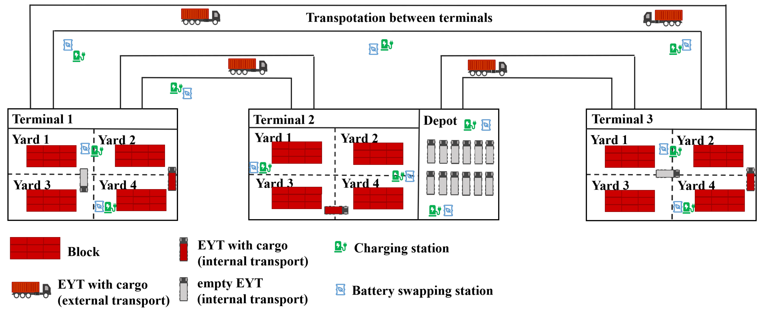
In this study, a planning problem related to horizontal transportation within a port consisting of multiple container terminals is considered. As depicted in Figure 1, a fleet of Electric Trucks (ETs) is tasked with the collection and distribution of bulk goods across the terminals during the planning horizon [0, $T_{max}$]. The ETs depart from the depot with a fully charged battery and return after visiting their designated customers. Due to the limited battery capacity, the ETs have a restricted driving range, necessitating charging activities when they lack sufficient energy to complete their routes. In accordance with the current technology, these ETs are equipped with swappable batteries that can be recharged or replaced when depleted. Three recharging options are available for the ETs at each station: normal recharging, fast recharging, and battery swapping. Normal recharging and fast recharging involve replenishing the battery to ensure that the ET can continue serving subsequent customers. While normal recharging offers cost efficiency due to lower unit costs, it extends the station visit duration due to a slower recharging rate. The third option is battery swapping, which is characterized by a significantly shorter operational time compared to the route’s travel time. Irrespective of the current battery charge level, a fully charged battery replaces the existing one. Consequently, this alternative incurs higher costs than typical recharging methods due to its substantial electrical infrastructure requirements and more expensive equipment.

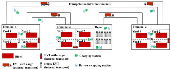
Figure 1. The ET work scene and container flows.

Let I and 0 denote the set of customers and the depot, respectively. Given that each recharging station allows multiple visits and can function, we define E as the set comprising all Charging Stations (CSs) and Battery Swapping Stations (BSSs), and their duplicates. Then, the problem can be represented by a complete graph $G=(V,A)$, where $V=I\cup E\cup \left\{0\right\}$ and $A=\left\{\right(i,j\left)\right|i,j\in V\}$. Each customer $i\in I$ is associated with a demand $q_i$, a service time $s_i$, and a predetermined soft time window $[{\underline{w}}_i$, ${\overline{w}}_i)$. Specifically, an ET must wait if it arrives at a customer point before the specified early arrival time ${\underline{w}}_i$ or incur a delay penalty cost if it arrives later than the preferred latest arrival time ${\overline{w}}_i$. In addition, when the ET traverses any arc $(i,j)\in A$, it incurs a travel time $t_{ij}$ as well as an energy cost $e_{ij}$ due to battery discharging. The mathematical notation is given in Table 2.

Table 2. Mathematical notations.

Sets
A	Set of arc (i, j), $i,j\in V$
$E^c$	Set of recharging stations
$E^s$	Set of battery swapping stations
E	Set of recharging and battery swapping stations ($E^c\cup E^s$)
I	Set of customers
V	Set of nodes ($I\cup E\cup \left\{0\right\})$
Parameters
$a_i^{k,m}$	Charging time for each breakpoint k, based on nonlinear charging function, $k\in K$,
	$i\in E^c$, $m\in M$
$b_i^{k,m}$	Charge level for each breakpoint k, based on nonlinear charging function, $k\in K$,
	$i\in E^c$, $m\in M$
C	Cargo capacity of a vehicle
$e_{i,j}$	Energy cost from node i to node j
$q_i$	Demand of customer i, $i\in I$
$Q^e$	Battery capacity of a vehicle, $Q^e\gg ma{x}_{i\in I,j\in E,j^{{}^{\prime }}\in E\cup \left\{0\right\}}\{e_{j,i}+e_{i,j^{{}^{\prime }}}\}$
$r^s$	Battery swapping time
$s_i$	Time required to serve customer i, $i\in I$
$t_{i,j}$	Travel time from node i to node j
$u_v$	Per unit fixed vehicle cost
$u_b$	Per unit energy cost
$u_d$	Per delay arrival penalty cost
$u_o$	Per unit cost of a vehicle occupying a charging station
$u_c^m$	Per unit cost of charging using mode m, $m\in M$
$u_s$	Cost per battery swap
v	Constant traveling speed of the vehicles
$[{\underline{w}}_i$, ${\overline{w}}_i)$	Soft time window of customer i, $i\in I$
Variables
${\underline{\beta }}_{i,j}$ / ${\overline{\beta }}_{i,j}$	the charge level when the ET arrives at and departs from $j\in E^c$, respectively, $x_{i,j}$ = 1
${\underline{c}}_{i,j}$ / ${\overline{c}}_{i,j}$	the time required to replenish the charge level from 0 to ${\underline{\beta }}_{i,j}$ / ${\overline{\beta }}_{i,j}$, respectively
${\Delta }_{i,j}$	the time spent at $j\in E$, $x_{i,j}$ = 1
${\eta }_i$	delay arrival time at customer i
${\gamma }_{i,j}$	the charge level when a vehicle departs from node i, $(i,j)\in A$, $x_{i,j}$ = 1
$l_{i,j}$	remaining cargo when a vehicle departs from node i, $(i,j)\in A$, $x_{i,j}$ = 1
${\tau }_{i,j}$	the time when a vehicle departs from node i, $(i,j)\in A$, $x_{i,j}$ = 1
$x_{i,j}$	1 if the vehicle traverses arc(i,j), 0 otherwise
${\underline{y}}_{i,j}^{m,k}$ / ${\overline{y}}_{i,j}^{m,k}$	1 if the charge level is between $a_i^{k-1,m}$ and $a_i^{k,m}$, when the ET arrives at and departs
	from $j\in E^c$, respectively, 0 otherwise, $x_{i,j}$ = 1
$z_{i,i^{{}^{\prime }}}$	1 if an ET starts from customer i, and serves customer $i^{{}^{\prime }}$ after passing through a
	station, otherwise 0
${\underline{\epsilon }}_{i,j}^{m,k}$ / ${\overline{\epsilon }}_{i,j}^{m,k}$	coefficients of the breakpoint $k\in K_m$ in the piecewise linear approximation when the
	ET arrives at and departs from $j\in E^c$ respectively, $x_{i,j}$ = 1
${\rho }_{i,j}^c$	charging costs of a vehicle at node $j\in E^c$, $x_{i,j}$ = 1

3.2. Assumptions

To formulate the mathematical model for the problem, we establish the following fundamental assumptions:

• A fixed number of homogeneous Electric Trucks (ETs), initially fully charged, are available at the central depot.
• The central depot and the charging stations operate continuously, allowing ETs to return to the depot at any time.
• ETs depart from the depot and eventually return to the depot.
• Each customer is visited exactly once by an ET, while multiple ETs can visit each CS or BS.
• ETs travel at a constant speed, and their batteries discharge at a linear rate solely in relation to the distance traversed.

3.3. Problem Formulation

Nonlinear Charging Function

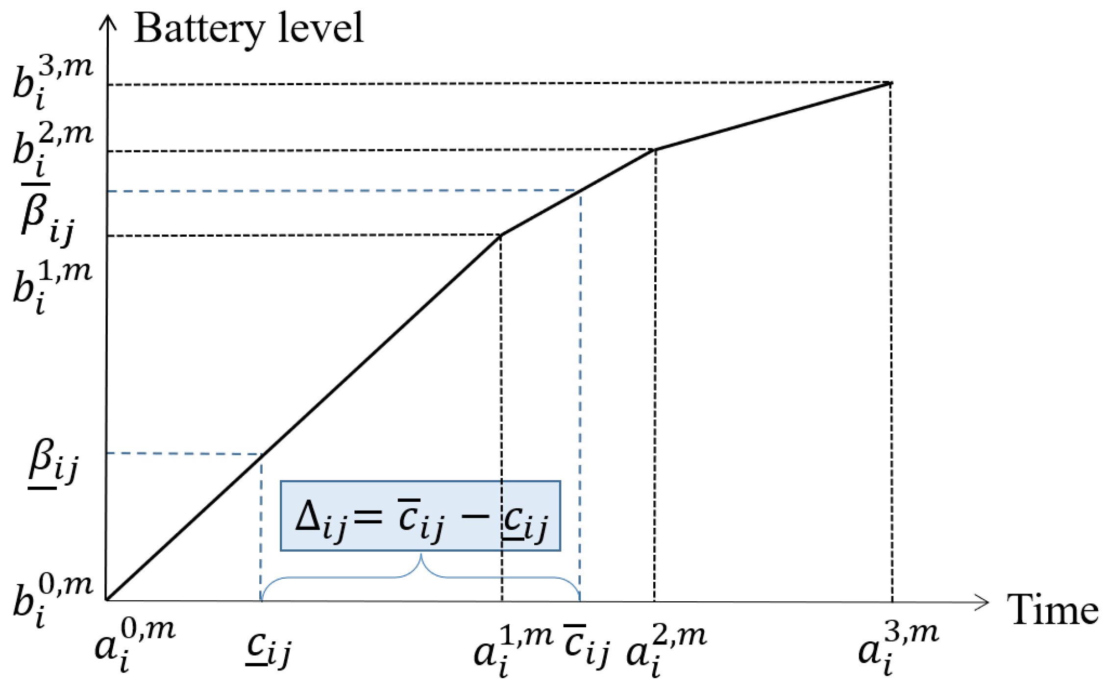
Before presenting the mathematical model, it is essential to elaborate on the nonlinear charging function. Let $m\in M$ denote the charging options, where $M=\{0,1,2\}$ represents normal charging, fast charging, and battery swapping, respectively. The nonlinear charging function proposed by Montoya et al. [10] is adopted in this study. For each CS as $i\in E^c$, a corresponding piecewise linear approximation charging function $F_i^m\left(t\right)$ is defined, as shown in Figure 2. $F_i^m\left(t\right)$ consists of four sets of coordinate points $\left\{(a_i^{k,m},b_i^{k,m})\right\}$, indicating the time $a_i^{k,m}$ required for the ET to replenish its charge from 0 to $b_i^{k,m}$. The input parameters $F_i^m\left(t\right)$ are the remaining charge ${\underline{\beta }}_{i,j}$ when the ET arrives at the CS and the remaining charge ${\overline{\beta }}_{i,j}$ when it leaves the CS. Then the time ${\Delta }_{i,j}$ consumed by the ET at the CS can be expressed as $F_i^{m^{-1}}\left({\overline{\beta }}_{i,j}\right)-F_i^{m^{-1}}\left({\underline{\beta }}_{i,j}\right)$. To construct a mixed-integer programming model, this paper introduces binary decision variables ${\underline{y}}_{i,j}^{m,k}$ and ${\overline{y}}_{i,j}^{m,k}$ to track the charging status of ETs. Specifically, ${\underline{y}}_{i,j}^{m,k}$ = 1 if the ET arrives at the CS with a charge between $b_i^{k-1,m}$ and $b_i^{k,m}$, while ${\overline{y}}_{i,j}^{m,k}$ = 1 if the ET leaves the CS with a charge in the range of $b_i^{k-1,m}$ and $b_i^{k,m}$. In addition, continuous decision variables ${\underline{\epsilon }}_{i,j}^{m,k}$ and ${\overline{\epsilon }}_{i,j}^{m,k}$ are introduced to represent $({\underline{c}}_{i,j},{\underline{\beta }}_{i,j})$ and $({\overline{c}}_{i,j},{\underline{\beta }}_{i,j})$ as linear combinations of $\left\{(a_i^{k,m},b_i^{k,m})\right\}$, respectively.

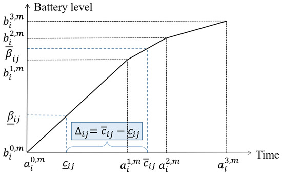
Figure 2. Piecewise linear approximation function.

Figure 3 depicts an example of an EVRP considering a nonlinear partial charging and swapping strategy. The example involves ten customer nodes and three CS or BSS nodes. The values $[{\gamma }_{i,j},{\tau }_{i,j},l_{i,j}]$ on the nodes indicate the remaining charge, current time, and remaining cargo when the ET leaves from that node, respectively. The values $(e_{i,j},t_{i,j})$ on the arcs indicate the energy and time consumed by the ET while traversing the arcs. Upon arriving at customer node $C_3$, the ET is required to wait until the specified time window is open before unloading due to time constraints. Therefore, the departure time from this node is calculated based on the earliest start time of service plus the service time, as opposed to the arrival time plus the service time. When the ET’s battery is running low, it has the option to recharge at a nearby CS ($C_3\to C{S}_1\to C_7,C_1\to C{S}_2\to C_6$) or to visit a BSS ($C_2\to BS{S}_1\to C_0$) for battery replacement. CSs offer two modes of charging, normal and fast, each with its own piecewise linear approximate charging function. In the provided example, the ET arrives at $C{S}_1$ with a remaining charge of ${\underline{\beta }}_{i,j}$ = 38.8 and replenishes the charge to ${\overline{\beta }}_{i,j}$ = 69.0 to meet operational requirements. The function indicates that the corresponding charging times for ${\underline{\beta }}_{i,j}$ and ${\overline{\beta }}_{i,j}$ are ${\underline{c}}_{i,j}$ = 19.4 and ${\overline{c}}_{i,j}$ = 36.9, respectively. Therefore, the total time spent at $C{S}_1$ will be ${\Delta }_1$ = 36.9 − 19.4 = 17.5.

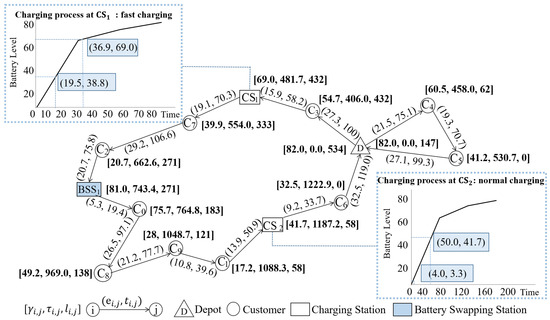
Figure 3. An example of electric truck driving path.

3.4. Mathematical Model

3.4.1. Objective Function

Satisfying the demand of all customers, the objective of our model is to minimize the total costs including fixed costs, energy costs, delay penalty costs, charging costs, and battery swapping costs.

• Fixed Costs: the fixed cost required to dispatch an ET including the total costs of truck purchase, truck maintenance, employee salaries, opportunity costs, and other expenses allocated to the unit truck. Let $x_{0,i}=1$, representing the trucks driving from the depot to customer i, and ${\displaystyle \sum _{(0,i)\in A}}{x}_{0,i}$, indicating the total number of vehicles departing from the depot. With a per unit fixed vehicle cost $u_v$, the total fixed costs of dispatched ETs are then

  $$T{C}_1=u_v\sum _{(0,i)\in A}{x}_{0,i}$$

  (1)
• Energy Costs: the costs of energy consumed by ETs while driving. Let $e_{i,j}$ represent the energy costs by vehicles from node i to node j, which is linearly related to driving distance. With per unit energy cost $u_b$, the total energy costs generated by driving can be expressed as

  $$T{C}_2=u_b\sum _{(i,j)\in A}{e}_{i,j}{x}_{i,j}$$

  (2)
• Delay Penalty Costs: the penalty costs paid by ETs for exceeding the latest service time specified by customers during the process of unloading. A specific expression being provided in constraint (21), ${\eta }_i$ represents delay arrival time at customer i. With per unit delay penalty cost $u_d$, the total delay penalty costs generated on the serving route are then

  $$T{C}_3=u_d\sum _{i\in I}{\eta }_i$$

  (3)
• Charging Costs: the costs of ETs replenishing energy at CSs on account of insufficient charge level. With a specific expression in constraint (35), ${\rho }_{i,j}^c$ represents the cost of a vehicle traversing $arc(i,j)\in A$ and recharging at CS $j\in E^c$, comprising two parts, that is, CS occupancy cost and basic electricity fee. The total charging costs during driving are formulated as

  $$T{C}_4=\sum _{j\in E^c}\sum _{(i,j)\in A}{\rho }_{i,j}^c$$

  (4)
• Battery Swapping Costs: the costs of ETs replacing the battery at BSS due to insufficient charge level. Unlike CSs, ETs replace fully charged batteries at the BSS, without having to pay for electricity based on the amount of charge. With per battery swap cost $u_s$, the total battery swapping costs generated by driving are then

  $$T{C}_5=u_s\sum _{j\in E^s}\sum _{(i,j)\in A}{x}_{i,j}$$

  (5)
• Overall, the objective function of this model can be formulated as

  $$Minimize{u}_v\sum _{(0,i)\in A}{x}_{0,i}+u_b\sum _{(i,j)\in A}{e}_{i,j}{x}_{i,j}+u_d\sum _{i\in I}{\eta }_i+\sum _{j\in E^c}\sum _{(i,j)\in A}{\rho }_{i,j}^c+u_s\sum _{j\in E^s}\sum _{(i,j)\in A}{x}_{i,j}$$

  (6)

3.4.2. Constraints

Based on the notation definitions and model assumptions mentioned above, this section classifies and models the real constraints involved in the problem, mainly including basic constraints, load capacity constraints, time constraints, battery capacity constraints, charging or swapping constraints, as well as valid inequalities and decision variables.

• Basic Constraints and Core Decisions
  Constraints (7)–(14) are typical constraints on the path conditions of the EVRP problem [22]. Specifically, constraint (7) ensures that each customer is visited by a truck exactly once. Constraint (8) guarantees the flow conservation between nodes. Constraints (9) and (10) ensure that the last and next nodes of a customer node be a depot, charging station, battery swapping station, or other customer, respectively. Constraints (11) and (12) connect decision variables $x_{i,j}$, $xj,i$, and $Z_{i,i^{{}^{\prime }}}$ (i.e., the next node of customer i and the last node of customer $i^{{}^{\prime }}$ must belong to CSs or BSSs when $z_{i,i^{{}^{\prime }}}$ is equal to 1). Constraint (13) represents that $x_{i,j}$ and $x_{j,i^{{}^{\prime }}}$ must be equal to 1 when $z_{i,i^{{}^{\prime }}}$ is equal to 1 (i.e., the ET departs from customer i and continues to serve customer j after replenishing the battery at a CS or BSS). The consistency of the accessed CS or BSS is ensured by constraint (14).

  $$\sum _{(i,j)\in A}{x}_{i,j}=1\forall i\in I$$

  (7)

  $$\sum _{(j,i)\in A}{x}_{j,i}-\sum _{(i,j)\in A}{x}_{i,j}=0\forall i\in V$$

  (8)

  $$x_{0,i^{{}^{\prime }}}\sum _{i\in I,i\ne i^{{}^{\prime }}}{z}_{i,i^{{}^{\prime }}}+\sum _{i\in I,i\ne i^{{}^{\prime }}}{x}_{i,i^{{}^{\prime }}}=1\forall i^{{}^{\prime }}\in I$$

  (9)

  $$x_{i,0}\sum _{i^{{}^{\prime }}\in I,i^{{}^{\prime }}\ne i}{z}_{i,i^{{}^{\prime }}}+\sum _{i^{{}^{\prime }}\in I,i^{{}^{\prime }}\ne i}{x}_{i,i^{{}^{\prime }}}=1\forall i\in I$$

  (10)

  $$\sum _{(i,j)\in A,j\in E}{x}_{i,j}=\sum _{i^{{}^{\prime }}\in I,i^{{}^{\prime }}\ne i}{z}_{i,i^{{}^{\prime }}}\forall i\in I$$

  (11)

  $$\sum _{(j,i^{{}^{\prime }})\in A,j\in E}{x}_{j,i^{{}^{\prime }}}=\sum _{i\in I,i\ne i^{{}^{\prime }}}{z}_{i,i^{{}^{\prime }}}\forall i^{{}^{\prime }}\in I$$

  (12)

  $$\sum _{(i,j)\in A,j\in E}{x}_{i,j}+\sum _{(j,i^{{}^{\prime }})\in A,j\in E}{x}_{j,i^{{}^{\prime }}}\ge 2z_{i,i^{{}^{\prime }}}\forall i,i^{{}^{\prime }}\in I,i\ne i^{{}^{\prime }}$$

  (13)

  $$\mid V\mid (z_{i,i^{{}^{\prime }}}-1)\le \sum _{(i,j)\in A,j\in E}j{x}_{i,j}-\sum _{(j,i^{{}^{\prime }})\in A,j\in E}j{x}_{j,i^{{}^{\prime }}}\le \mid V\mid (1-z_{i,i^{{}^{\prime }}})\forall i,i^{{}^{\prime }}\in I,i\ne i^{{}^{\prime }}$$

  (14)
• Load Capacity Constraints
  Constraint (15) is about the load capacity constraint for ETs [35]. Constraint (16) indicates that the remaining cargo capacity of ETs at each customer node should be able to meet the demand. Constraints (17) and (18) ensure that the remaining cargo capacity of an ET does not change when passing through a CS or BSS (i.e., CS or BSS have no demand for goods).

  $$0\le l_{i,j}\le C{x}_{i,j}\forall (i,j)\in A,i\in V$$

  (15)

  $$0\le \sum _{(i,j)\in A}{l}_{i,j}=\sum _{(j,i)\in A}(l_{j,i}-q_i{x}_{j,i})\forall i\in I$$

  (16)

  $$\sum _{(i,j)\in A,j\in E}{l}_{i,j}\ge \sum _{(j,i^{{}^{\prime }})\in A,j\in E}{l}_{j,i_{{}^{\prime }}}-C(1-z_{i,i^{{}^{\prime }}})\forall i,i^{{}^{\prime }}\in I,i\ne i^{{}^{\prime }}$$

  (17)

  $$\sum _{(i,j)\in A,j\in E}{l}_{i,j}\le \sum _{(j,i^{{}^{\prime }})\in A,j\in E}{l}_{j,i_{{}^{\prime }}}+C(1-z_{i,i^{{}^{\prime }}})\forall i,i^{{}^{\prime }}\in I,i\ne i^{{}^{\prime }}$$

  (18)
• Time Constraints
  Constraint (19) links decision variables $x_{i,j}$ with ${\tau }_{i,j}$. Constraint (20) restricts the time at which ETs leave each customer node under the condition of time windows and service time. The delay arrival time of each customer node is defined by constraint (21). Constraints (22) and (23) express the time spent at CSs and BSSs, respectively. Constraint (24) tracks the time at which ETs depart from each customer node. Also, constraints (25) and (26) track the time at which ETs depart from each CS or BSS.

  $$\tau \le T_{max}{x}_{i,j}\forall (i,j)\in A,i\in I\cup E$$

  (19)

  $${\underline{w}}_i+s_i\le \sum _{(i,j)\in A}{\tau }_{i,j}\forall i\in I$$

  (20)

  $${\eta }_i\ge \sum _{(i,j)\in A}{\tau }_{i,j}-s_i-{\overline{w}}_i\forall i\in I$$

  (21)

  $${\Delta }_{i,j}={\overline{c}}_{i,j}-{\underline{c}}_{i,j}\forall (i,j)\in A,j\in E^c$$

  (22)

  $${\Delta }_{i,j}=r^s{x}_{i,j}\forall (i,j)\in A,j\in E^s$$

  (23)

  $$\sum _{(j,i)\in A}({\tau }_{j,i}+(t_{j,i}+s_i)x_{j,i})\le \sum _{(i,j)\in A}{\tau }_{i,j}\forall i\in I$$

  (24)

  $$\sum _{(i,j)\in A,j\in E}({\tau }_{i,j}+t_{i,j}{x}_{i,j}+{\Delta }_{i,j}\ge \sum _{(j,i^{{}^{\prime }})\in A,j\in E}{\tau }_{j,i^{{}^{\prime }}}-T_{max}(1-z_{i,i^{{}^{\prime }}})\forall i,i^{{}^{\prime }}\in I,i\ne i^{{}^{\prime }}$$

  (25)

  $$\sum _{(i,j)\in A,j\in E}({\tau }_{i,j}+t_{i,j}{x}_{i,j}+{\Delta }_{i,j}\le \sum _{(j,i^{{}^{\prime }})\in A,j\in E}{\tau }_{j,i^{{}^{\prime }}}+T_{max}(1-z_{i,i^{{}^{\prime }}})\forall i,i^{{}^{\prime }}\in I,i\ne i^{{}^{\prime }}$$

  (26)
• Battery Capacity Constraints
  Constraints (27) and (28) link decision variables $x_{i,j}$ and ${\gamma }_{i,j}$. Specifically, the range of charge level for ETs departing from customer and station nodes is provided by constraint (27), and constraint (28) ensures that ETs depart from the depot and BSSs with full batteries. Constraints (29) and (30) track the charge level when an ET departs from each customer node and arrives at charging station j. Constraints (31) and (32) track the charge level when an ET departs from a CS to serve the next customer node. Constraint (33) represents that if an ET accesses a CS or BSS, it must replenish more electricity than it consumes while driving, that is, avoiding invalid access.

  $$e_{i,j}{x}_{i,j}\le {\gamma }_{i,j}\le Q^e{x}_{i,j}\forall (i,j)\in A,i\in I\cup E^c$$

  (27)

  $${\gamma }_{i,j}=Q^e{x}_{i,j}\forall (i,j)\in A,i\in E^s\cup \left\{0\right\}$$

  (28)

  $$\sum _{(i,j)\in A}{\gamma }_{i,j}-\sum _{(i,j)\in A}{e}_{i,j}{x}_{i,j}=\sum _{(j,j^{{}^{\prime }})\in A}{\gamma }_{j,j^{{}^{\prime }}}\forall j\in I$$

  (29)

  $$\sum _{(i,j)\in A,j\in E^c}{\gamma }_{i,j}-\sum _{(i,j,j\in E^c)\in A}{e}_{i,j}{x}_{i,j}=\sum _{(i,j)\in A,j\in E^c}{\underline{\beta }}_{i,j}\forall i\in I$$

  (30)

  $$\sum _{(j,i^{{}^{\prime }})\in A,j\in E^c}{\gamma }_{j,i^{{}^{\prime }}}\le \sum _{(i,j)\in A,j\in E^c}{\overline{\beta }}_{i,j}+Q^e(1-z_{i,i^{{}^{\prime }}})\forall i,i^{{}^{\prime }}\in I,i\ne i^{{}^{\prime }}$$

  (31)

  $$\sum _{(j,i^{{}^{\prime }})\in A,j\in E^c}{\gamma }_{j,i^{{}^{\prime }}}\ge \sum _{(i,j)\in A,j\in E^c}{\overline{\beta }}_{i,j}-Q^e(1-z_{i,i^{{}^{\prime }}})\forall i,i^{{}^{\prime }}\in I,i\ne i^{{}^{\prime }}$$

  (32)

  $$\begin{array}{cc}\hfill & \sum _{(i,j)\in A,j\in E^c}({\overline{\beta }}_{i,j}-{\underline{\beta }}_{i,j})+Q^e\sum _{(i,j)\in A,j\in E^s}{x}_{i,j}\ge \sum _{(i,j)\in A,j\in E^c}{x}_{i,j}{e}_{i,j}\hfill \\ \hfill & +\sum _{(j,i^{{}^{\prime }})\in A,j\in E}{x}_{j,i^{{}^{\prime }}}{e}_{j,i^{{}^{\prime }}}-(1-x_{i,i^{{}^{\prime }}})e_{i,i^{{}^{\prime }}}+2Q^e(z_{i,i^{{}^{\prime }}}-1)\forall i,i^{{}^{\prime }}\in I,i\ne i^{{}^{\prime }}\hfill \end{array}$$

  (33)
• Charging and Swapping Constraints
  Constraint (34) indicates that the ET arrives at the CS with a battery level no higher than that at the time of departure. Constraint (35) defines the charging costs, which include both the time cost of occupying the CS and the basic electricity cost for charging. Based on the piecewise linear approximation charging function, constraints (36)–(43) define the charge level and the corresponding time for an ET to arrive at a CS, and represent $({\underline{c}}_{i,j},{\underline{\beta }}_{i,j})$ as a convex combination of $(a_j^{m,k},b_j^{m,k})$ by introducing a charging coefficient ${\underline{\epsilon }}_{i,j}^{m,k}$. Similarly, constraints (44)–(51) define the battery level and the corresponding time for an ET to depart from a CS, and represent $({\overline{c}}_{i,j},{\overline{\beta }}_{i,j})$ as a convex combination of $(a_j^{m,k},b_j^{m,k})$ by introducing a charging coefficient ${\overline{\epsilon }}_{i,j}^{m,k}$. Constraint (52) ensures charging consistency when entering and leaving CSs for ETs.

  $${\underline{\beta }}_{i,j}\le {\overline{\beta }}_{i,j}\forall (i,j)\in A,j\in E^c$$

  (34)

  $${\rho }_{i,j}^c=u_o{\Delta }_{i,j}+\sum _{m\in M}\sum _{k\in K_m}({\overline{\epsilon }}_{i,j}^{m,k}-{\underline{\epsilon }}_{i,j}^{m,k})b_j^{m,k}{u}_c^m\forall (i,j)\in A,j\in E^c$$

  (35)

  $${\underline{\beta }}_{i,j}=\sum _{m\in M}\sum _{k\in K_m}{\underline{\epsilon }}_{i,j}^{m,k}{b}_j^{m,k}\forall (i,j)\in A,j\in E^c$$

  (36)

  $${\underline{c}}_{i,j}=\sum _{m\in M}\sum _{k\in K_m}{\underline{\epsilon }}_{i,j}^{m,k}{a}_j^{m,k}\forall (i,j)\in A,j\in E^c$$

  (37)

  $$\sum _{m\in M}\sum _{k\in K_m}{\underline{\epsilon }}_{i,j}^{m,k}=x_{i,j}\forall (i,j)\in A,j\in E^c$$

  (38)

  $$\sum _{m\in M}\sum _{k\in K_m\setminus \left\{0\right\}}{\underline{y}}_{i,j}^{m,k}=x_{i,j}\forall (i,j)\in A,j\in E^c$$

  (39)

  $$\sum _{k\in K_m\setminus \left\{0\right\}}{\underline{y}}_{i,j}^{m,k}\le x_{i,j}\forall (i,j)\in A,j\in E^c,m\in M$$

  (40)

  $${\underline{\epsilon }}_{i,j}^{m,0}\le {\underline{y}}_{i,j}^{m,1}\forall (i,j)\in A,j\in E^c,m\in M$$

  (41)

  $${\underline{\epsilon }}_{i,j}^{m,k}\le {\underline{y}}_{i,j}^{m,k}+{\underline{y}}_{i,j}^{m,k+1}\forall (i,j)\in A,j\in E^c,m\in M,k\in K_m\setminus \{0,\mid K_m\mid \}$$

  (42)

  $${\underline{\epsilon }}_{i,j}^{m,\mid K_m\mid }\le {\underline{y}}_{i,j}^{m,\mid K_m\mid }\forall (i,j)\in A,j\in E^c,m\in M$$

  (43)

  $${\overline{\beta }}_{i,j}=\sum _{m\in M}\sum _{k\in K_m}{\overline{\epsilon }}_{i,j}^{m,k}{b}_j^{m,k}\forall (i,j)\in A,j\in E^c$$

  (44)

  $${\overline{c}}_{i,j}=\sum _{m\in M}\sum _{k\in K_m}{\overline{\epsilon }}_{i,j}^{m,k}{a}_j^{m,k}\forall (i,j)\in A,j\in E^c$$

  (45)

  $$\sum _{m\in M}\sum _{k\in K_m}{\overline{\epsilon }}_{i,j}^{m,k}=x_{i,j}\forall (i,j)\in A,j\in E^c$$

  (46)

  $$\sum _{m\in M}\sum _{k\in K_m\setminus \left\{0\right\}}{\overline{y}}_{i,j}^{m,k}=x_{i,j}\forall (i,j)\in A,j\in E^c$$

  (47)

  $$\sum _{k\in K_m\setminus \left\{0\right\}}{\overline{y}}_{i,j}^{m,k}\le x_{i,j}\forall (i,j)\in A,j\in E^c,m\in M$$

  (48)

  $${\overline{\epsilon }}_{i,j}^{m,0}\le {\overline{y}}_{i,j}^{m,1}\forall (i,j)\in A,j\in E^c,m\in M$$

  (49)

  $${\overline{\epsilon }}_{i,j}^{m,k}\le {\overline{y}}_{i,j}^{m,k}+{\overline{y}}_{i,j}^{m,k+1}\forall (i,j)\in A,j\in E^c,m\in M,k\in K_m\setminus \{0,\mid K_m\mid \}$$

  (50)

  $${\overline{\epsilon }}_{i,j}^{m,\mid K_m\mid }\le {\overline{y}}_{i,j}^{m,\mid K_m\mid }\forall (i,j)\in A,j\in E^c,m\in M$$

  (51)

  $$\sum _{k\in K_m\setminus \left\{0\right\}}{\overline{y}}_{i,j}^{m,k}\ge \sum _{k\in K_m\setminus \left\{0\right\}}{\underline{y}}_{i,j}^{m,k}\forall (i,j)\in A,j\in E^c,m\in M$$

  (52)
• Valid Inequalities and Decision Variables
  Constraint (53) ensures that the ET has enough electricity power to complete the service and return to the depot. Constraint (54) defines the minimum remaining power for an ET to depart from each customer node. Specifically, when $z_{i,i^{{}^{\prime }}}$ is equal to 1, the remaining power to reach customer node $i^{{}^{\prime }}$ must not be less than that at customer node i plus the power replenished at a CS or BSS minus the power consumed en route. Constraints (55)–(61) define the range of decision variables.

  $$\sum _{i\in V}\sum _{(i,j)\in A}{x}_{i,j}{e}_{i,j}\le Q^e(\sum _{(0,i)\in A}{x}_{0,i}+\sum _{i\in I}\sum _{(i,j)\in A,j\in E^s}{x}_{i,j})+\sum _{i\in I}\sum _{(i,j)\in A,j\in E^c}({\overline{\beta }}_{i,j}-{\underline{\beta }}_{i,j})$$

  (53)

  $$\begin{array}{cc}\hfill & \sum _{(i,j)\in A}{\gamma }_{i,j}-\sum _{(i^{{}^{\prime }},j)\in A}{\gamma }_{i^{{}^{\prime }},j}+\sum _{j\in E^c}({\overline{\beta }}_{i,j}-{\underline{\beta }}_{i,j})+Q^e\sum _{j\in E^s}{x}_{i,j}\ge x_{i,i^{{}^{\prime }}}{e}_{i,i^{{}^{\prime }}}\hfill \\ \hfill & +\sum _{(i,j)\in A,j\in E}{x}_{i,j}{e}_{i,j}+\sum _{(j,i^{{}^{\prime }})\in A,j\in E}{x}_{j,i^{{}^{\prime }}}{e}_{j,i^{{}^{\prime }}}+3Q^e(z_{i,i^{{}^{\prime }}}-1)\forall i,i^{{}^{\prime }}\in I,i\ne i^{{}^{\prime }}\hfill \end{array}$$

  (54)

  $$x_{i,j}\in \{0,1\},{\tau }_{i,j}\ge 0,{\gamma }_{i,j}\ge 0,l_{i,j}\ge 0\forall (i,j)\in A$$

  (55)

  $${\underline{y}}_{i,j}^{m,k}\in \{0,1\},{\overline{y}}_{i,j}^{m,k}\in \{0,1\}\forall (i,j)\in A,j\in E^c,m\in M,k\in K_m\setminus \left\{0\right\}$$

  (56)

  $${\underline{\epsilon }}_{i,j}^{m,k}\ge 0,{\overline{\epsilon }}_{i,j}^{m,k}\ge 0\forall (i,j)\in A,j\in E^c,m\in M,k\in K_m$$

  (57)

  $${\underline{\beta }}_{i,j}\ge 0,{\overline{\beta }}_{i,j}\ge 0,{\underline{c}}_{i,j}\ge 0,{\overline{c}}_{i,j}\ge 0\forall (i,j)\in A,j\in E^c$$

  (58)

  $${\Delta }_{i,j}\ge 0\forall (i,j)\in A,j\in E$$

  (59)

  $${\eta }_i\ge 0\forall i\in I$$

  (60)

  $$z_{i,i^{{}^{\prime }}}\in \{0,1\}\forall i,i^{{}^{\prime }}\in I,i\ne i^{{}^{\prime }}$$

  (61)

4. Solution Heuristic

In a recent study by Qin et al. (2021) [36], the authors identified the limitations of exact methods for solving EVRPs, and demonstrated that the ALNS algorithm outperformed other existing heuristics in the literature. Motivated by these findings, an ALNS algorithm was developed to solve our problem. Given the presence of multiple charging options and nonlinear charging functions, tailored destroy-and-repair operators are designed. For comparison, this paper also implemented the ALNS for solving an EVRP as introduced by Keskin et al. [33], denoted by Pre-ALNS.

The ALNS algorithm uses multiple removal and insertion operators and dynamically selects the operator to execute in each iteration by roulette selection operation [37]. The selection depends on the historical operator performance, i.e., operators with better historical performance have a higher probability of being selected. The weight of an operator in the nth iteration is calculated as follows:

$$w_a^n=(1-\rho )w_a^{n-1}+\rho \frac{{\pi }_a^{n-1}}{{\theta }_a^{n-1}},$$

(62)

where $\rho \in [0,1]$ represents the speed of weight adjustment based on the operator’s performance, and ${\theta }_a^{n-1}$ and ${\pi }_a^{n-1}$ indicate the number of uses of the operator a and its score in the n−1th cycle, respectively. The probability of selecting each operator in iteration cycle n is given by

$$P_a^n=\frac{w_a^n}{{\displaystyle \sum _{l=1}^m}{w}_l^n}.$$

(63)

Note that the proposed ALNS algorithm consists of four different sets of operators: customer removal, station removal, customer insertion, and station insertion. Each operator set’s adaptive weights and selection probabilities are calculated independently, alongside differing iteration cycles for customer and station nodes. Additionally, a probabilistic jumping technique is utilized, derived from the simulated annealing algorithm, to randomly search for the global optimal solution within the solution space. The adaptive weights and selection probabilities of each operator set are calculated separately, and the iteration cycles for customer nodes and station nodes are different. In addition, we introduce the probabilistic jumping from the simulated annealing algorithm to find the global optimal solution randomly in the solution space. Figure 4 presents the ALNS algorithm flow for the problem under study, in which $N_{RR}$ and $N_{SR}$ represent the number of iteration times to select the RR operator and SR operator, respectively. $n_r$, $n_{RR}$, and $N_{max}$ denote the current internal iteration times, the max internal iteration times, and the max iteration times.

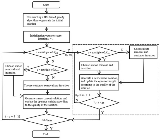
Figure 4. The ALNS algorithm flow suitable for the problem studied in this paper.

4.1. Removal Operators

The removal operator is a vital component of the ALNS, which significantly affects the solution quality. The degree of destruction caused by the removal operator directly determines the algorithm’s effectiveness in exploring the solution space. If the removal operator is less destructive, the algorithm may not explore the solution space thoroughly enough. Conversely, if the operator excessively destroys the current solution, the solution quality degrades, needing more time to converge. Given the different impacts of removing customer nodes and station nodes on the current solution, we apply separate Customer Removal (CR) and Station Removal (SR) operators to destroy the current solution.

4.1.1. Customer Removal

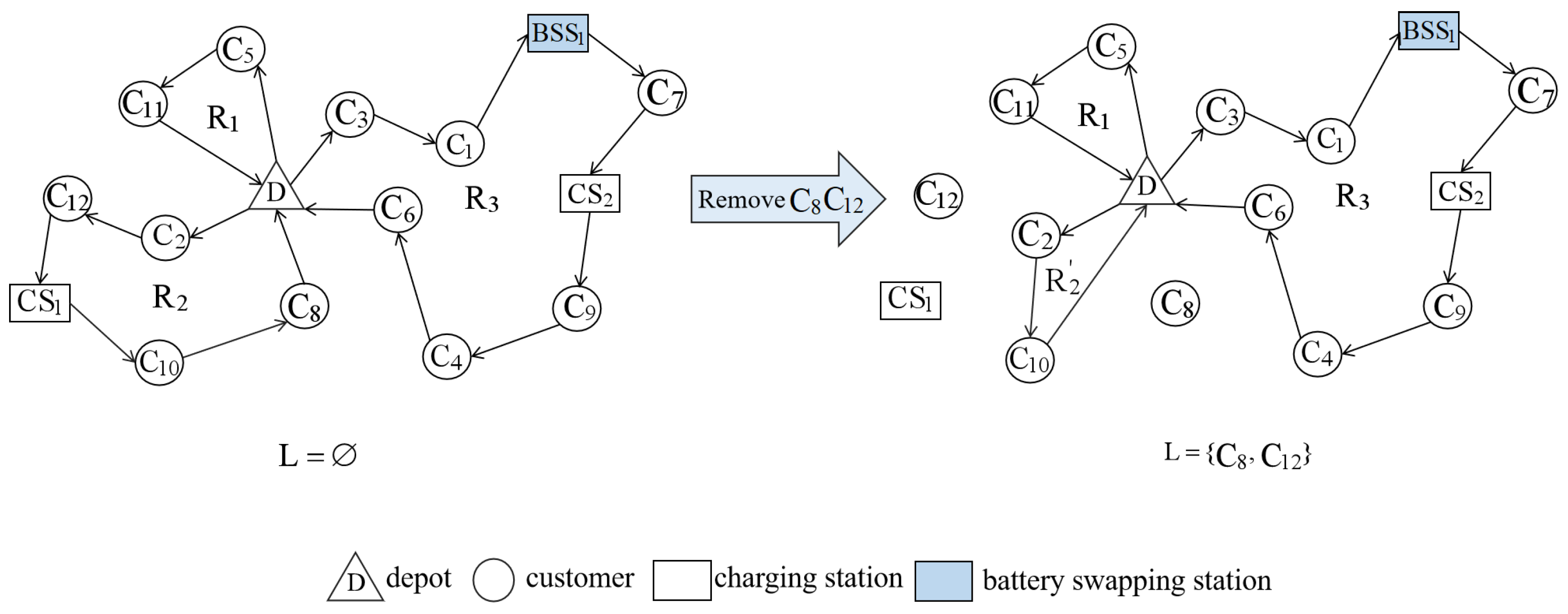
Figure 5 illustrates the implementation process of the customer removal operator. In addition to commonly used CR heuristics, such as Random [38], Worst Distance [38], Worst cost [15], and Worst Delay-Time Removal [39], we utilize the following operators tailored to the problem’s characteristics, inspired by previous research [38,40]:

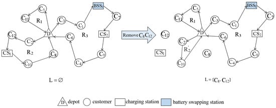
Figure 5. The implementation process of customer node removal operator.

• Related Customer Removal (ReCR): In ReCR, we remove a set of customer nodes with high correlation. These nodes are easily exchanged during subsequent iterations and eliminated from the current solution. A similarity function is constructed to express the correlation of customer nodes:

  $$R(i,j)={\mathsf{\Phi }}_1{d}_{i,j}+{\mathsf{\Phi }}_2\mid ({\overline{w}}_i-{\underline{w}}_i)-({\overline{w}}_j-{\underline{w}}_j)\mid +{\mathsf{\Phi }}_3{\theta }_{i,j},$$

  (64)

  where ${\mathsf{\Phi }}_1$, ${\mathsf{\Phi }}_2$, and ${\mathsf{\Phi }}_3\in [0,1]$ represent correlation coefficient with ${\mathsf{\Phi }}_1+{\mathsf{\Phi }}_2+{\mathsf{\Phi }}_3=1$; $d_{i,j}$ denotes the distance between customers i and j; ${\overline{w}}_i$ and ${\overline{w}}_j$ represent the earliest service times of customers i and j, respectively; ${\underline{w}}_i$ and ${\underline{w}}_j$ represent the latest service times of customers i and j; ${\theta }_{i,j}$ indicates whether customers i and j are on the same route (${\theta }_{i,j}$ = −1 if on the same route; ${\theta }_{i,j}$ = 1, otherwise). A smaller value of $R(i,j)$ means higher relevance between the two customers. The function calculates the similarity between customer node i and other customer nodes j which have been inserted into the route. Then, the customers are sorted in non-decreasing order based on this similarity. In addition, a related customer removal factor is used to introduce randomness during the removal process. Customer nodes are successively removed based on the similarity between them until $n_{cr}$ customer nodes are removed.
• Worst Wait-Time Removal (WWTR): Due to the presence of time windows, vehicles must wait until the time window opens if they arrive early. Therefore, the WWTP operator is applied to remove the customer nodes with long waiting times from the current solution. This allows vehicles to arrive within the customer service time window as frequently as possible.
• Station-Based Removal (SBR): To reduce the charging and swapping costs of the current solution, we employ the SBR operator to remove the customer nodes connected to the charging and swapping station nodes. This reduction results in fewer vehicles passing through these stations. The heuristic framework is presented in Algorithm 1.

Algorithm 1 Station-Based Removal(SBR)

1: Initialization: number of customer nodes to be removed $n_{cr}$; $n\leftarrow 0$ 2: while n < $n_{cr}$ do 3:    Calculate the number of station nodes for all routes in the solution $staNum\left(r\right)$ 4:    if $staNum\left(r\right)$ > 0 then 5:      Save route r into the set tempRoute 6:    end if 7:    Randomly select the route $r^{*}$ to be destroyed from the set $staNum\left(r\right)$ 8:    Randomly select a station node sta from the route $r^{*}$ 9:    Remove the station node sta and the customer node k connected to sta 10:    Put the customer node k into the removal list L 11:    if The power of route $r^{*}$ is not feasible then 12:      Repair route r using GSI 13:    end if 14:    Clear the set tempRoute 15:    $n++$ 16: end while

4.1.2. Station Removal

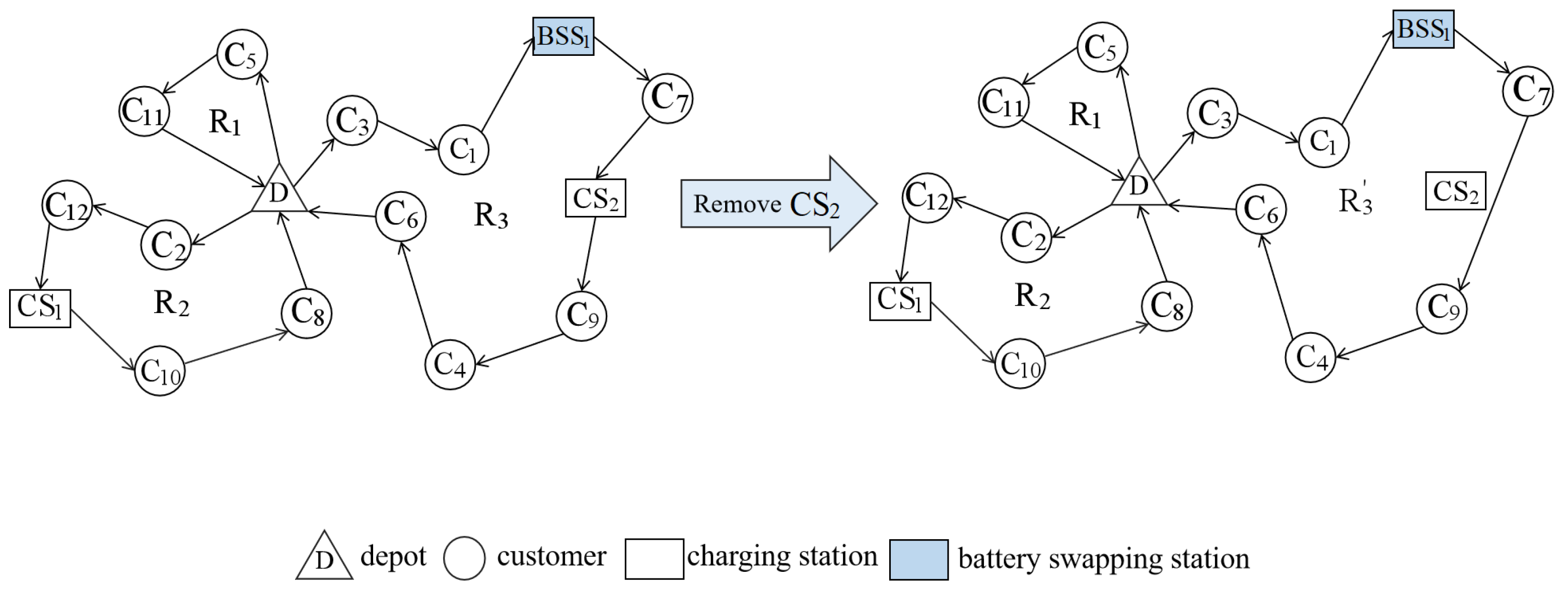
The EVRP involves the removing or reordering of station nodes. This permutation has the potential to enhance the solution obtained. Following each $N_{SR}$ iteration, the algorithm dynamically selects a station removal operator and removes $n_{sr}$ station nodes from the current solution according to the destroy rules of the operator. The value of $n_{sr}$ is determined by the total number of charging and swapping stations $n_s$ in the current solution ($n_{s}r=min(10,0.4n_s)$). Figure 6 shows the implementation process of the node removal operator of the CS or swapping station.

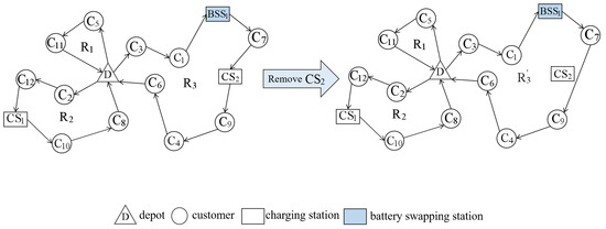
Figure 6. The implementation process of station node removal operator.

In addition to the Random Station Removal (RSR) operator proposed by Keskin and Catay [31] and the Expensive Station Removal (ESR) [32], we introduce two additional Station Removal (SR) operators inspired by previous research concepts:

• Worst Distance Station Removal (WDSR) [16]: Similar to the WDR mechanism, WDSR removes station nodes that cause considerable detours in the current solution, thereby reducing energy consumption. The removal cost of station j is defined as

  $$c(i,j)=d_{(}i,j)+d_{(}j,i+1)-d_{(}i,i+1),$$

  (65)

  where $d_{i,j}$ and $d_{i,j}$ represent the distances from customer i to station j and from j to customer $i+1$, respectively.
• Least Used Station Removal (LUSR) [41]: For ETs that can be replenished with as much power as possible at stations, LUSR removes the CS or swapping stations with the least additional power for ETs from the current solution, rather than making multiple visits for small amounts of charging. This reduces the cost associated with frequent vehicle access to stations.

4.1.3. Route Removal

After each $N_{RR}$ iteration, our algorithm performs $n_{RR}$ times random route removal operator [42] or greedy route removal operator [31]. This process selects $n_{rr}$ routes, removes all nodes within the routes, and performs these removals according to the operator-specified rules. The value of $n_{rr}$ depends on the total number of routes, $n_r$, and is randomly generated within the interval $[0.1n_r,0.4n_r]$. Figure 7 shows the effects of the route removal operator when $n_{rr}=2$.

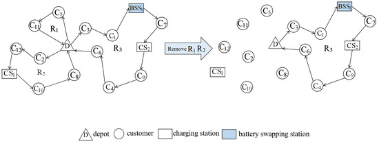
Figure 7. The implementation process of route removal operator.

4.2. Insertion Operators

After removing some customer and station nodes from the current solution, the algorithm utilizes the insertion operators to reinsert these nodes into the routes. Thereby, we design specific customer insertion and station insertion operators to repair the damaged solution.

4.2.1. Customer Insertion

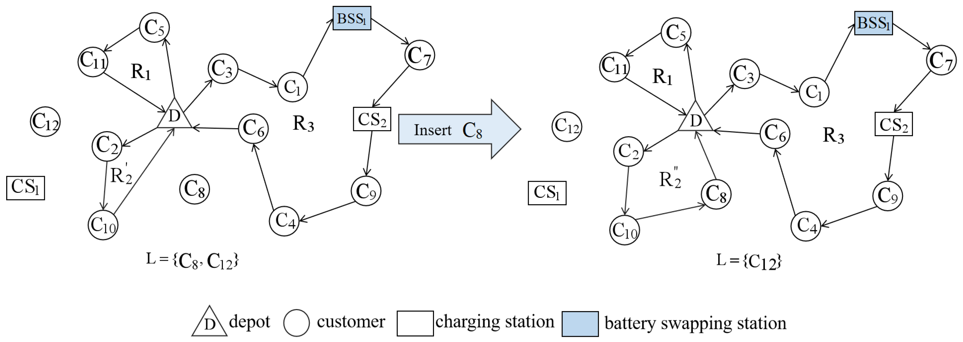
After each CR operator, our algorithm adaptively selects a Customer Insertion (CI) operator. Following operator-specified rules, the CI operator reinserts the customer nodes from the removal list L into the routes and simultaneously removes them from the list. The value of $n_{rr}$ depends on the total number of routes $n_r$ and is randomly generated on the interval $[0.1n_r,0.4n_r]$. The implementation process of the CI operator is presented in Figure 8.

Figure 8. The implementation process of customer insertion operator.

We use Random Customer Insertion (RCI) and Greedy Customer Insertion (GCI) as proposed by Keskin and Catay [31]. Regret-K Customer Insertion (RKCI) [15] is also employed, with values of k = 2 and k = 3. Considering the presence of various time-related costs, such as delay costs and charging costs, we introduce Time-based Customer Insertion (TCI) to minimize the total duration of vehicle routes. It continuously inserts the customer node with the minimum route time variation into better positions.

4.2.2. Station Insertion

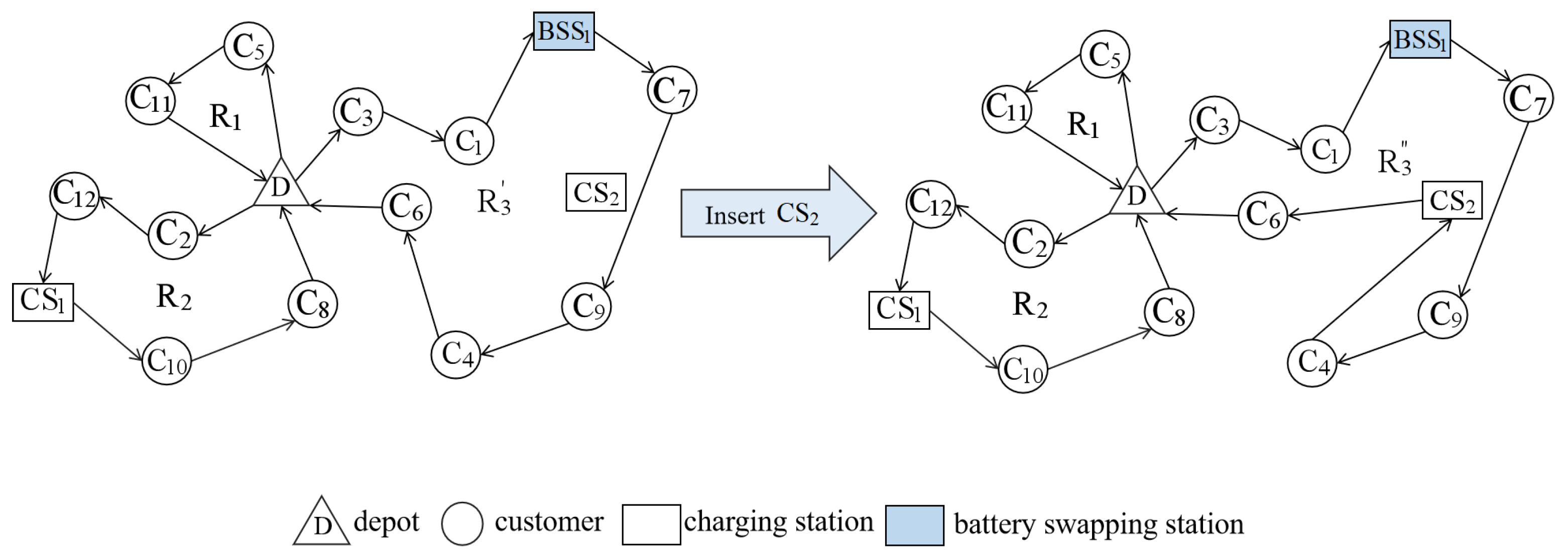
After removing station nodes, some routes may become infeasible due to battery capacity limitations. Hence, it is necessary to reinsert the stations to restore the feasibility of the routes. For an infeasible route, the algorithm identifies the first customer node with a negative charge level when the vehicle arrives, and then adaptively selects a Station Insertion (SI) operator. Since partial charging is considered, the amount of electricity replenished by the vehicle at the CS should be able to meet the energy requirements of the subsequent route. Note that the redundant CSs that do not provide power are removed after repairing the route by inserting the CSs. Figure 9 outlines the implementation process of the SI operator.

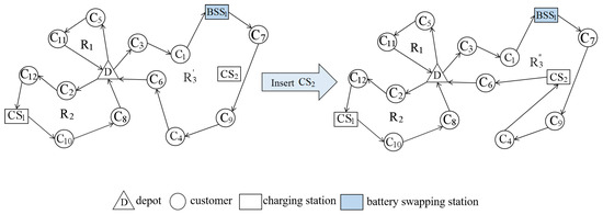
Figure 9. The implementation process of station insertion operator.

Greedy Station Insertion (GSI) [43] is adopted. It selects the nearest station to the first customer node with a negative charge level when the vehicle arrives as the insertion point, and chooses the mode $m\in M$ to minimize the cost. In addition to GSI, we design two additional SI operators:

• Minimum Cost Insertion (MCI): The MCI operator considers inserting the station node into the first arc and its previous arc where the EV has a negative charge level. It then chooses the insertion point with the lowest insertion cost, including the determination of the charging rate. Algorithm 2 presents the heuristic framework of MCI.

  Algorithm 2 Minimum Cost Insertion (MCI)

  1: Initialization: the number of routes in the current solution routeNum; $r\leftarrow 0$; $k\leftarrow 0$; $\Delta d=d_{i-1,j}+d_{i,j}$; $c_{pos,m}=c_{pos,m}^d+c_{pos,m}^c$; $c_{pos}^{*}=mi{n}_{m\in M}\left\{c_{pos,m}\right\}+c_{pos}^{*}=+\infty$ 2: while r < routeNum do 3:    while The power of route r is not feasible do 4:      Find the first customer node with negative power and record its location p 5:      for p-k > 0 do 6:         Calculate the distance $\Delta d$ between the customer with a location of $po{s}_1$ = p-k and all station nodes 7:         if The electric quantity of the vehicle arriving at the charging station node $s_1$ is less than 0 then 8:           $\mathit{k}++$ 9:         else 10:           Calculate the minimum insertion cost $c_{po{s}_1}^{*}$ at the insertion node $s_1$ 11:           Jump out of the current cycle 12:         end if 13:      end for 14:      Calculate the distance $\Delta d$ between the customer node of the location $po{s}_2$ = $po{s}_1$-1 and all the station nodes 15:      Record the station node $s_2$ corresponding to min($\Delta d$) 16:      Calculate the minimum insertion cost $c_{po{s}_2}^{*}$ at the insertion node $s_2$ 17:      if $c_{po{s}_1}^{*}$ < $c_{po{s}_2}^{*}$ then 18:         Insertion $s_1$ at position $po{s}_1$ 19:      else 20:         Insertion $s_2$ at position $po{s}_2$ 21:      end if 22:    end while 23:    r++ 24: end while 25: Delete redundant station nodes

• Best Location Insertion (BLI): The BLI operator expands the search range, considering all the insertable locations (pos) between the first customer node with negative power and the previously visited station node or depot. It identifies the best station insertion method as follows. Firstly, it selects the station closest to pos, calculates the insertion cost of using different modes $m\in M$ at the station, and figures out the best station with the minimum cost. Subsequently, it inserts the nearest station along with the determined mode into the arc between the location and the previous customer node. The heuristic framework of BLI is provided in Algorithm 3.

4.3. Constructing the Initial Solution

Because of the sensitivity of ALNS to the initial solution, we design an initial solution generation algorithm based on a greedy fashion. Although the greedy insertion algorithm does not guarantee finding the global optimal solution, it can efficiently produce a suitable initial solution. Various station-related decisions are involved in the problem, including CS location, charging mode, and supplementary power, which have a great impact on the quality of the initial solution and subsequent iterative optimization. Thus, a greedy initial solution generation algorithm based on the BLI is proposed similar to the greedy insertion algorithm for customer nodes.

Algorithm 3 Best Location Insertion (BLI)

1: Initialization: the number of routes in the current solution routeNum; $r\leftarrow 0$; $k\leftarrow 0$; $\Delta d=d_{i-1,j}+d_{i,j}$; $c_{pos,m}=c_{pos,m}^d+c_{pos,m}^c$; $c_{pos}^{*}=mi{n}_{m\in M}\left\{c_{pos,m}\right\}+c_{pos}^{*}=+\infty$ 2: while r < routeNum do 3:    while The power of route r is not feasible do 4:      Find the first customer node with negative power and record its location p 5:      for p-k > 0 do 6:         Calculate the distance $\Delta d$ between the customer with a location of $po{s}_1$ = p-k and all station nodes 7:         Record the station node s corresponding to min($\Delta d$) 8:         Save the position pos, station s, and insertion cost $c_{pos}^{*}$ to the set tempSta 9:         k++ 10:      end for 11:      Sort the set tempSta according to the monotonicity of $c_{pos}^{*}$ 12:      Insert the station $s^{*}$ with index 0 in set tempSta into the corresponding position $po{s}^{{}^{\prime }}$ 13:    end while 14:    r++ 15: end while 16: Delete redundant station nodes

4.4. Simulated Annealing Acceptance Criterion

In the heuristic algorithm, it is necessary to evaluate whether the obtained solution can be accepted as the current solution or not. The simplest way is to accept only solutions better than the current one. Nevertheless, such a setting increases the possibility of falling into a local optimum. To tackle this issue, we used the probabilistic acceptance mechanism of the simulated annealing algorithm [44]. This mechanism occasionally accepts less competitive solutions, allowing the algorithm to escape the local optimum and explore the solution space more extensively.

5. Numerical Experiments and Analysis of the Model

5.1. Instance Generation and Parameter Setting

To evaluate the performance of the ALNS algorithm and its practical applicability, a series of numerical experiments are conducted based on a modified dataset inspired by the Montoya et al. [10] dataset (https://pan.baidu.com/s/1IWPKF4pjyBMuSrGyai7z-w?pwd=1x7a, accessed on 29 August 2023). In this part, the construction of instances used in this study is described, including node coordinates, service time windows, and customer goods demand. The details are summarized as follows:

• This paper uses the information of customer and station node coordinates provided by Montoya et al. [10], distributed within a 120 km × 120 km range. To accommodate practical scenarios, we opted for 10 and 20 customer nodes from the dataset for small-scale experiments, while 40, 80, 100, and 120 customer nodes were chosen for large-scale experiments. The locations of BSSs correspond to those of CSs, ranging from 2 to 21 stations in each set of instances.
• Customer service time windows are generated using a uniform distribution method. The earliest service start time ranges from 6 a.m. to 8 p.m., represented as ${\underline{w}}_i\in uniform$ [360, 1200] on the timeline. The time window widths range from 1 to 2 hours, expressed as $t{w}_i\in \mathit{uniform}$ [60, 120] on the timeline. The latest service start time is calculated as

  $${\overline{w}}_i={\underline{w}}_i+t{w}_i.$$

  (66)
• Customer cargo demand is generated using the uniform distribution method, with $q_i$ randomly generated in the interval uniform [10, 100].

In summary, 12 datasets are generated based on the number of customer and station nodes, resulting in a total of 72 instances. To facilitate the experimental analysis, each instance is named as Gm-n, where m and n denote the dataset number and instance number, respectively. The dataset sizes are presented in Table 3.

Table 3. Experimental data size setting.

Dataset Number	NC 1	NCS 2	Dataset Number	NC	NCS
G1	10	2	G7	80	8
G2	10	3	G8	80	12
G3	20	3	G9	100	12
G4	20	4	G10	100	16
G5	40	5	G11	120	16
G6	40	8	G12	120	21

¹ NC: Number of customers ² NCS: Number of charging stations.

Several process parameters are considered to ensure the rapid convergence and efficient resolution of the ALNS algorithm. These parameters, which include operator score increments, simulated annealing control parameters, correlation coefficients, operator removal factors, and iteration counts. Among them, iteration count parameters are adopted with reference to Keskin and Çatay’s work [32]. And the other parameters are determined experimentally based on the problem. The detailed parameter values are provided in Appendix A (Table A1).

5.2. Validation of Algorithm Effectiveness

The following section presents the results of numerical experiments conducted on both small- and large-scale instances. Given the complexity of the problem, the state-of-the-art commercial solver CPLEX is only practical for small-scale instances. For large-scale instances, we have implemented Pre-ALNS for comparison purposes. All experiments were conducted in a JAVA environment, utilizing CPLEX 12.6.1 as the MIP model solver, with a maximum solution time of 7200 s. The experiments were run on a computer configured as AMD Ryzen 7, 2.9 GHz CPU, 16 GB memory. To guarantee experiment consistency, the proposed ALNS algorithm and Pre-ALNS algorithm were each tested five times for every instance, and the best results were selected for further analysis.

5.2.1. Results for Small Instances

To validate our problem model and the effectiveness of the ALNS algorithm, we solve 24 small-scale instances using both the CPLEX solver and the ALNS algorithm. We then compare the results in terms of solution quality and efficiency. Table 4 and Table 5 present the results for small-scale settings (group G1 to group G4). These tables provide information on instances, the number of charging or swapping times (NR), total costs (TCs), running time (CPU(s)), differences between the numbers of charging or swapping times ($\Delta$N), and the gap (Gap %) between TCs obtained by CPLEX and the proposed ALNS. A positive Gap % signifies that the proposed ALNS solution outperforms the CPLEX solver, while the highlighted results indicate that the optimal solution is found by CPLEX.

Table 4. Comparison of results on small size instances (NC = 10).

Instance		CPLEX			ALNS			$\mathbf{\Delta }$N	Gap %
		NR	TC	CPU(s)	NR	TC	CPU(s)
G1	1	3	889.97	26.66	3	889.97	5.93	0	0.00
	2	2	1242.35	50.08	2	1242.35	3.98	0	0.00
	3	0	1154.71	36.44	0	1154.71	3.70	0	0.00
	4	2	1237.01	41.02	2	1237.01	4.08	0	0.00
	5	0	1129.26	27.86	0	1129.26	3.25	0	0.00
	6	2	1125.39	38.59	2	1125.39	5.10	0	0.00
G2	1	3	889.97	53.53	3	889.97	5.63	0	0.00
	2	2	1242.35	82.42	2	1242.35	3.89	0	0.00
	3	1	1145.87	303.08	1	1145.87	3.73	0	0.00
	4	2	1236.43	99.05	2	1236.43	4.07	0	0.00
	5	0	1129.26	42.84	0	1129.26	3.18	0	0.00
	6	2	1073.59	179.52	2	1073.59	3.93	0	0.00
Average		1.58	1124.68	81.76	1.58	1124.68	4.21	0	0.00

Table 5. Comparison of results on small size instances (NC = 20).

Instance		CPLEX			ALNS			$\mathbf{\Delta }$N	Gap %
		NR	TC	CPU(s)	NR	TC	CPU(s)
G3	1	1	1327.36	7200	1	1327.36	34.61	0	0.00
	2	3	1261.53	7200	3	1261.53	33.12	0	0.00
	3	2	1289.45	7200	2	1287.93	30.31	0	0.12
	4	2	1273.72	7200	2	1273.72	27.87	0	0.00
	5	2	1320.14	7200	2	1319.78	28.23	0	0.03
	6	2	1318.33	7200	2	1318.33	29.15	0	0.00
G4	1	3	1408.56	7200	1	1327.36	36.26	−2	5.76
	2	3	1260.43	7200	2	1258.62	31.28	−1	0.14
	3	2	1288.68	7200	2	1288.68	30.88	0	0.00
	4	3	1262.32	7200	3	1262.32	28.95	0	0.00
	5	2	1319.78	7200	2	1319.78	28.79	0	0.00
	6	3	1334.61	7200	2	1317.27	29.90	−1	1.30
Average		2.33	1305.41	7200	2.00	1296.89	30.78	−0.33	0.61

Table 4 reveals that the total costs and the number of charging or battery swapping times obtained by the two methods are identical. CPLEX succeeds in obtaining optimal solutions of all instances within the predefined maximum running time, indicating the optimality of the solution values. The ALNS algorithm achieves the same total costs as CPLEX, which signifies its performance in tackling the problem. Meanwhile, the running time of ALNS significantly outperforms that of CPLEX. Specifically, the time gap between the two methods notably increases with the expansion of customer size. On average, the proposed algorithm proves to be a significantly faster solution, with a speed advantage of approximately 20 times over the CPLEX method. Regarding Table 5, we find that the objective function values improved by an average of 0.61% compared to CPLEX for the test instances. For three instances of group G4, the ALNS outperforms CPLEX in terms of objective function values, with fewer charging operations. This may be due to the fact that inefficient charging plans would incur additional energy consumption costs and operational times, and thus lead to higher total distribution costs. Additionally, the ALNS still exhibits a short average running time of 30.78 s, while CPLEX reaches the maximum setting time.

5.2.2. Results for Large Instances

The previous section has confirmed the performance of the ALNS algorithm in solving small-scale problems. In order to further test its computational capabilities for large-scale problems, this section solves the instance groups G5 to G12. The objective is to assess the quality and efficiency of the solutions generated. The ALNS algorithm has been widely adopted for addressing VRP variants [9,45,46]. Therefore, to demonstrate the enhanced efficacy of our algorithm, a comparison with the Pre-ALNS is conducted. For each instance, both the proposed ALNS and Pre-ALNS algorithms are run five times, and the best results are selected for comparative analysis.

Table 6 provides a summary of the average results for the Pre-ALNS and ALNS algorithms applied to large-scale instances. In this table, $Ga{p}_c$ represents the difference in the objective function values, while $Ga{p}_t$ indicates the difference in runtime. Positive values for both $Ga{p}_c$ and $Ga{p}_t$ signify that the ALNS algorithm outperforms the Pre-ALNS algorithm in terms of solution quality and efficiency. The detailed results are provided in Appendix B (Table A2).

Table 6. The summary of average results of the Pre-ALNS and ALNS on large-size instances.

ID	Pre-ALNS			ALNS			$\mathbf{\Delta }$N	${\mathbf{Gap}}_{\mathbf{c}}$ (%)	${\mathbf{Gap}}_{\mathbf{t}}$ (%)
	NR	TC	CPU(s)	NR	TC	CPU(s)
G5&6	4.67	2120.71	289.72	3.92	2093.72	286.17	−0.75	1.26	1.24
G7&8	5.42	2957.77	1507.41	4.67	2864.61	1505.68	−0.75	3.05	−0.27
G9&10	7.08	3541.30	2738.73	5.67	3407.49	2731.95	−1.42	3.73	0.23
G11&12	9.58	4293.02	3998.15	7.50	4092.65	4007.96	−2.08	4.67	−0.26

As shown in Table 6, the proposed ALNS outperforms the Pre-ALNS in terms of total cost. By applying the proposed ALNS, cost savings range from 1.26% to 4.67% across the four test groups. Moreover, the superiority of the proposed ALNS becomes more pronounced as the instance size increases. When analyzing the outcomes of both algorithms, it is observable that the developed algorithm effectively minimizes costs by optimizing charging and battery swapping frequencies. In terms of running time, both methods exhibit efficiency. The proposed solution approach solved some instance groups with a shorter average solution time. Overall, our methodology displays improved performance in solving the problem to a certain extent.

5.3. Sensitivity Analysis and Managerial Insights

To evaluate the impact of various factors on our model, we conduct three sets of experiments. These experiments aim to analyze how partial charging strategy, nonlinear charging functions, and battery swapping strategy influence the total cost, number of vehicles, and charging/battery swapping times. These experimental instances are randomly selected from 12 instance groups. The results of these comparisons are summarized in Table 7, Table 8 and Table 9, with corresponding visualizations provided in Figure 10, Figure 11 and Figure 12. Detailed comparisons are provided in Appendix C (Table A3, Table A4 and Table A5). In the tables, we define the following notations: TC for the total cost, DC for delay penalty cost, NV for the number of dispatched vehicles, NC for the number of visits to Charging Stations (CSs), NB for the number of visits to Battery Swapping Stations (BSSs), and $\Delta X$ to denote cost or quantity differences.

Table 7. Experimental results under full charging strategy and partial charging strategy.

Instance	Full Charging					Partial Charging
	TC	DC	NV	NC	NB	TC	DC	NV	NC	NB
G1-6	1129.3	0	2	0	0	1125.4	289.4	1	1	1
G2-1	941.4	51.7	1	1	1	890.0	51.7	1	2	1
G3-4	1323.0	0	2	0	1	1273.7	0	2	2	0
G4-1	1327.4	0	2	0	1	1327.4	0	2	0	1
G5-5	2191.4	0	3	1	2	2081.6	0	3	4	1
G6-5	2114.4	0	3	0	2	2068.5	0	3	3	1
G7-5	3051.7	0	4	0	4	2950.3	1.9	4	5	2
G8-2	2828.7	0	4	0	3	2683.8	12.0	4	3	1
G9-5	3358.2	81.8	5	1	1	3187.7	0	5	2	1
G10-1	3663.9	0	5	0	4	3570.5	0	5	1	3
G11-4	4350.1	0	6	0	5	4104.3	11.2	6	7	1
G12-5	4377.1	0	6	0	5	4201.8	1.1	6	7	2

Table 8. Experimental results under linear and nonlinear charging function.

Instance	Linear Charging					Nonlinear Charging
	TC	DC	NV	NC	NB	TC	DC	NV	NC	NB
G1-6	1039.7	214.4	1	1	1	1125.4	298.4	1	1	1
G2-1	890.0	51.7	1	2	1	890.0	51.7	1	2	1
G3-4	1263.8	0	2	2	0	1273.7	0	2	2	0
G4-1	1327.4	0	2	0	1	1327.4	0	2	0	1
G5-5	2070.9	0	3	4	1	2081.6	0	3	4	1
G6-5	2049.1	0	3	3	1	2068.5	0	3	3	1
G7-5	2920.9	0	4	3	2	2950.3	1.9	4	5	2
G8-2	2672.5	0	4	3	1	2683.8	12.0	4	3	1
G9-5	3173.3	0	5	4	0	3187.7	0	5	1	3
G10-1	3532.4	0	5	5	2	3570.5	0	5	1	3
G11-4	4097.7	0	6	6	1	4104.3	11.2	6	7	1
G12-5	4148.6	0	6	7	1	4201.8	1.1	6	7	2

Table 9. Experimental results without and with battery swapping strategy.

Instance	Without Swapping					With Swapping
	TC	DC	NV	NC	NB	TC	DC	NV	NC	NB
G1-6	1129.3	0	2	0	0	1125.4	298.4	1	1	1
G2-1	929.7	62.7	1	3	0	890.0	51.7	1	2	1
G3-4	1273.7	0	2	2	0	1273.7	0	2	2	0
G4-1	1343.3	0	2	3	0	1327.4	0	2	0	1
G5-5	2203.8	14.3	3	5	0	2081.6	0	3	4	1
G6-5	2181.1	14.8	3	4	0	2068.5	0	3	3	1
G7-5	3024.1	3.7	4	8	0	2950.3	1.9	4	5	2
G8-2	3005.0	0	5	2	0	2683.8	12.0	4	3	1
G9-5	3234.4	56.1	5	6	0	3187.7	0	5	2	1
G10-1	3821.3	11.4	5	8	0	3570.5	0	5	1	3
G11-4	4458.5	10.6	7	6	0	4104.3	11.2	6	7	1
G12-5	4411.9	0	7	6	0	4201.8	1.1	6	7	2

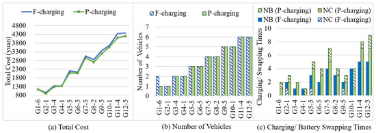
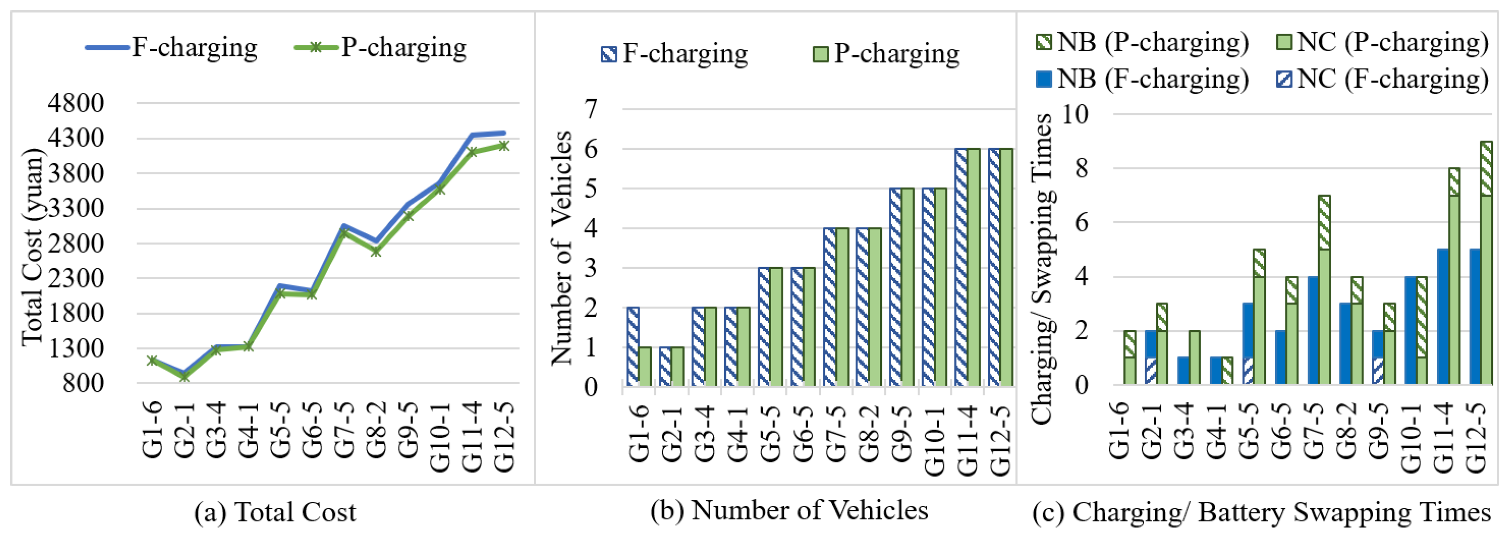
Figure 10. Comparison of results under full charging strategy and partial charging strategy. (a) Total cost. (b) Number of vehicles. (c) Charging or battery swapping times.

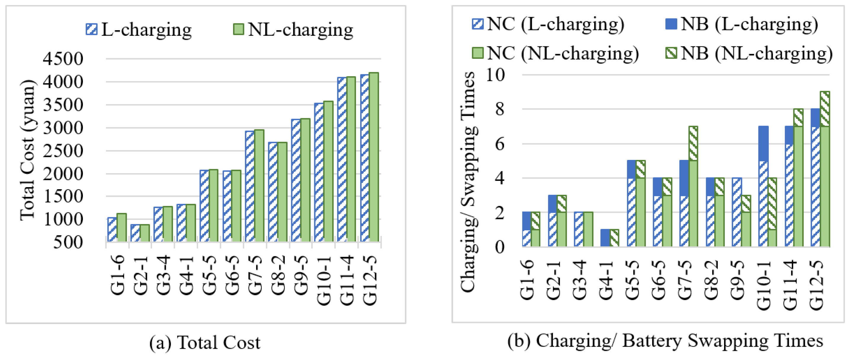
Figure 11. Comparison of results under linear and nonlinear function. (a) Total cost. (b) Charging or battery swapping times.

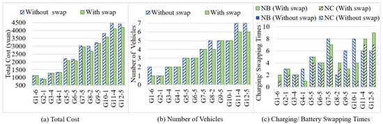
Figure 12. Comparison of results without and with battery swapping strategy. (a) Total cost. (b) Number of vehicles. (c) Charging or battery swapping times.

5.3.1. The Influence of Partial Charging Strategy

To analyze the impact of the partial charging strategy, experiments are conducted under both full charging and partial charging settings. The full charging strategy means that the trucks must replenish the battery to the full state at the CS.

Figure 10 illustrates the comparisons between the two charging strategies. Figure 10a clearly illustrates that the total operational cost under the partial charging strategy is consistently lower than that under the full charging strategy. Figure 10b indicates that the number of dispatched vehicles is mostly the same under both strategies, except for G1-6. Figure 10c presents evidence that allowing ETs to leave the CS with an appropriate level of charge can reduce visits to the Battery Swapping Station (BSS) in most scenarios, while increasing visits to the CS. This is due to the effectiveness of partial charging, which allows vehicles to recharge more quickly and reduces the need for battery swapping. Additionally, partial charging can lead to increased charging and swapping times and delay costs, but it can also lower the number of dispatched trucks and total operational costs, as seen in G1-6. Therefore, considering partial charging can enable port terminal operators to make optimal charging and swapping decisions, resulting in reduced operational costs across various scenarios.

5.3.2. Nonlinear Charging Impact Analysis

In this part, experiments are conducted in solving problem instances using linear and piecewise linear approximate charging functions. Figure 11 provides a visual comparison of the results in Table 8. Figure 11a demonstrates that nonlinear charging results in slightly higher total costs compared to linear charging. This is due to the piecewise linear charging function, which gradually reduces the charging rate as the battery level approaches full and charging time increases. As per Table 8, it is important to note that extended charging times may lead to delays and additional penalty costs, which are often underestimated by linear charging assumptions. In Figure 11b, we observe that ETs tend to opt for battery swapping mode to minimize delays, resulting in higher battery swapping costs. Therefore, port terminal operators should consider not only the single charging process but also the battery endurance mileage and allocate charging time based on the actual charging power of ETs to avoid such costs.

5.3.3. The Influence of Battery Swapping Strategy

To explore the impact of the battery swapping option on the routing solution, we also conducted experiments using the algorithm without considering battery swapping. Figure 12a shows that all instances obtain lower total costs when the battery swapping option is employed. Combined with Figure 12b,c, there may be two possible reasons. Firstly, the battery swapping mode allows ETs to rapidly reach a full charge level in a short period of time, which means each truck is allowed to serve more customers while satisfying the service time window. This leads to a reduction in the number of dispatched vehicles. Secondly, in distribution schemes with the same number of dispatched vehicles, the vehicle tends to choose battery swapping overcharging to reduce recharging frequency and the energy consumption cost caused by frequent bypassing of the CSs. Based on this analysis, battery-replaceable ETs may offer more cost advantages from an operational efficiency perspective. However, port operators must consider challenges related to fleet renewal, battery swapping facilities, and market support.

6. Conclusions

This study aims to facilitate the decision-making process of port operators to dispatch electric trucks (ETs) within a green port context. Motivated by realistic scenarios, the objective function includes decision-making elements such as fixed vehicle costs, energy consumption, and replenishment costs, as well as delay penalty costs. The problem constitutes a variant of the Electric Vehicle Routing Problem with Time Windows, incorporating battery swapping, nonlinear charging, and partial charging options. Practical constraints include path constraints, load constraints, time constraints, and power constraints. To solve this complex problem, we introduce an improved Adaptive Large Neighborhood Search (ALNS) algorithm with innovative operators.

The performance of the proposed algorithm is evaluated through comparisons of small-scale and large-scale problems. In addition, sensitivity analyses provide valuable insights for port operators:

-

Operators should allocate fleets and supplementary power based on customer demands, considering both fixed and operational costs of ETs.

-

Distribution plans should account for the actual charging power of ETs, i.e., reasonably estimate the battery mileage and allocate sufficient charging time.

-

Battery-replaceable ETs can reduce operational costs because of faster charging and reduced recharging frequency. However, fleet renewal, battery swapping facilities, and market support may pose challenges.

Future research could incorporate more realistic factors, such as uncertainty in traveling routes or charging processes. Additionally, integrating the algorithms with specific acceleration strategies could further improve the algorithm’s efficiency. Lastly, the retrofitting and deployment of battery-replaceable ETs could be an interesting research direction.

References

- Ritchie, H.; Roser, M.; Rosado, P. CO2 and Greenhouse Gas Emissions. Our World in Data, 2020. Available online: https://ourworldindata.org/co2-and-greenhouse-gas-emissions(accessed on 29 August 2023).
- United Nations Conference on Trade and Development. Review of Maritime Transport 2018; United Nations: New York, NY, USA, 2018. Available online: https://unctad.org/publication/review-maritime-transport-2018 (accessed on 29 August 2023).
- United Nations Conference on Trade and Development. Review of Maritime Transport 2022, 2022 ed.; United Nations: New York, NY, USA, 2022. Available online: https://unctad.org/publication/review-maritime-transport-2022 (accessed on 29 August 2023).
- Goodchild, A.; Mohan, K. The Clean Trucks Program: Evaluation of Policy Impacts on Marine Terminal Operations. Marit. Econ. Logist. 2008, 10, 393–408. [Google Scholar] [CrossRef]
- Clott, C.B.; Hartman, B.C. Clean trucks in California ports: Modelling emissions policy. Int. J. Shipp. Transp. Logist. 2013, 5, 449–462. [Google Scholar] [CrossRef]
- Nielsen, I.E.; Do, N.A.D.; Nguyen, V.D.; Nielsen, P.; Michna, Z. Reducing Truck Emissions in Import Operations at Container Terminal—A Case Study in a Singaporean Port. In Technology Management for Sustainable Production and Logistics; Springer: Berlin/Heidelberg, Germany, 2015; pp. 133–151. [Google Scholar] [CrossRef]
- Guan, C.; Liu, R. Container terminal gate appointment system optimization. Marit. Econ. Logist. 2009, 11, 378–398. [Google Scholar] [CrossRef]
- Li, J.; Wang, F.; He, Y. Electric Vehicle Routing Problem with Battery Swapping Considering Energy Consumption and Carbon Emissions. Sustainability 2020, 12, 10537. [Google Scholar] [CrossRef]
- Mao, H.; Shi, J.; Zhou, Y.; Zhang, G. The Electric Vehicle Routing Problem With Time Windows and Multiple Recharging Options. IEEE Access 2020, 8, 114864–114875. [Google Scholar] [CrossRef]
- Montoya, A.; Guéret, C.; Mendoza, J.E.; Villegas, J.G. The electric vehicle routing problem with nonlinear charging function. Transp. Res. Methodol. 2017, 103, 87–110. [Google Scholar] [CrossRef]
- Desaulniers, G.; Madsen, O.B.; Ropke, S. Chapter 5: The Vehicle Routing Problem with Time Windows. In Vehicle Routing; Springer US: Philadelphia, PA, USA, 2005; pp. 119–159. [Google Scholar] [CrossRef]
- Errico, F.; Desaulniers, G.; Gendreau, M.; Rei, W.; Rousseau, L.M. A priori optimization with recourse for the vehicle routing problem with hard time windows and stochastic service times. Eur. J. Oper. Res. 2016, 249, 55–66. [Google Scholar] [CrossRef]
- Li, G.; Li, J. An Improved Tabu Search Algorithm for the Stochastic Vehicle Routing Problem With Soft Time Windows. IEEE Access 2020, 8, 158115–158124. [Google Scholar] [CrossRef]
- Küçükoğlu, İ.; Dewil, R.; Cattrysse, D. Hybrid simulated annealing and tabu search method for the electric travelling salesman problem with time windows and mixed charging rates. Expert Syst. Appl. 2019, 134, 279–303. [Google Scholar] [CrossRef]
- Zhao, M.; Lu, Y. A Heuristic Approach for a Real-World Electric Vehicle Routing Problem. Algorithms 2019, 12, 45. [Google Scholar] [CrossRef]
- Kancharla, S.R.; Ramadurai, G. An Adaptive Large Neighborhood Search Approach for Electric Vehicle Routing with Load-Dependent Energy Consumption. Transp. Dev. Econ. 2018, 4, 10. [Google Scholar] [CrossRef]
- Masmoudi, M.A.; Hosny, M.; Demir, E.; Genikomsakis, K.N.; Cheikhrouhou, N. The dial-a-ride problem with electric vehicles and battery swapping stations. Transp. Res. Part E Logist. Transp. Rev. 2018, 118, 392–420. [Google Scholar] [CrossRef]
- Zhou, B.H.; Tan, F. Electric vehicle handling routing and battery swap station location optimisation for automotive assembly lines. Int. J. Comput. Integr. Manuf. 2018, 31, 978–991. [Google Scholar] [CrossRef]
- Jie, W.; Yang, J.; Zhang, M.; Huang, Y. The two-echelon capacitated electric vehicle routing problem with battery swapping stations: Formulation and efficient methodology. Eur. J. Oper. Res. 2019, 272, 879–904. [Google Scholar] [CrossRef]
- Lam, E.; Desaulniers, G.; Stuckey, P.J. Branch-and-cut-and-price for the Electric Vehicle Routing Problem with Time Windows, Piecewise-Linear Recharging and Capacitated Recharging Stations. Comput. Oper. Res. 2022, 145, 105870. [Google Scholar] [CrossRef]
- Cataldo-Díaz, C.; Linfati, R.; Escobar, J.W. Mathematical Model for the Electric Vehicle Routing Problem Considering the State of Charge of the Batteries. Sustainability 2022, 14, 1645. [Google Scholar] [CrossRef]
- Felipe, Á.; Ortuño, M.T.; Righini, G.; Tirado, G. A heuristic approach for the green vehicle routing problem with multiple technologies and partial recharges. Transp. Res. Part E Logist. Transp. Rev. 2014, 71, 111–128. [Google Scholar] [CrossRef]
- Park, H.; Jin, S. Electric Vehicle Routing Problem with Heterogeneous Vehicles and Partial Charge. Int. J. Ind. Eng. Manag. 2020, 11, 215–225. [Google Scholar] [CrossRef]
- Jiang, M.; Zhang, Y.; Zhang, Y. Multi-Depot Electric Bus Scheduling Considering Operational Constraint and Partial Charging: A Case Study in Shenzhen, China. Sustainability 2022, 14, 255. [Google Scholar] [CrossRef]
- Akbay, M.A.; Kalayci, C.B.; Blum, C. Application of cmsa to the electric vehicle routing problem with time windows, simultaneous pickup and deliveries, and partial vehicle charging. In Proceedings of the Metaheuristics International Conference, Syracuse, Italy, 11–14 July 2022; pp. 1–16. [Google Scholar] [CrossRef]
- Verma, A. Electric vehicle routing problem with time windows, recharging stations and battery swapping stations. EURO J. Transp. Logist. 2018, 7, 415–451. [Google Scholar] [CrossRef]
- Amiri, A.; Zolfagharinia, H.; Amin, S.H. Routing a mixed fleet of conventional and electric vehicles for urban delivery problems: Considering different charging technologies and battery swapping. Int. J. Syst. Sci. Oper. Logist. 2023, 10, 2191804. [Google Scholar] [CrossRef]
- Froger, A.; Mendoza, J.E.; Jabali, O.; Laporte, G. Improved formulations and algorithmic components for the electric vehicle routing problem with nonlinear charging functions. Comput. Oper. Res. 2019, 104, 256–294. [Google Scholar] [CrossRef]
- Lee, C. An exact algorithm for the electric-vehicle routing problem with nonlinear charging time. J. Oper. Res. Soc. 2021, 72, 1461–1485. [Google Scholar] [CrossRef]
- Karakatič, S. Optimizing nonlinear charging times of electric vehicle routing with genetic algorithm. Expert Syst. Appl. 2021, 164, 114039. [Google Scholar] [CrossRef]
- Keskin, M.; Çatay, B. Partial recharge strategies for the electric vehicle routing problem with time windows. Transp. Res. Part C Emerg. Technol. 2016, 65, 111–127. [Google Scholar] [CrossRef]
- Keskin, M.; Çatay, B. A matheuristic method for the electric vehicle routing problem with time windows and fast chargers. Comput. Oper. Res. 2018, 100, 172–188. [Google Scholar] [CrossRef]
- Keskin, M.; Laporte, G.; Çatay, B. Electric Vehicle Routing Problem with Time-Dependent Waiting Times at Recharging Stations. Comput. Oper. Res. 2019, 107, 77–94. [Google Scholar] [CrossRef]
- Sayarshad, H.R.; Mahmoodian, V. An intelligent method for dynamic distribution of electric taxi batteries between charging and swapping stations. Sustain. Cities Soc. 2021, 65, 102605. [Google Scholar] [CrossRef]
- Afroditi, A.; Boile, M.; Theofanis, S.; Sdoukopoulos, E.; Margaritis, D. Electric Vehicle Routing Problem with Industry Constraints: Trends and Insights for Future Research. Transp. Res. Procedia 2014, 3, 452–459. [Google Scholar] [CrossRef]
- Qin, H.; Su, X.; Ren, T.; Luo, Z. A review on the electric vehicle routing problems: Variants and algorithms. Front. Eng. Manag. 2021, 8, 370–389. [Google Scholar] [CrossRef]
- Yu, F.; Fu, X.; Li, H.; Dong, G. Improved Roulette Wheel Selection-Based Genetic Algorithm for TSP. In Proceedings of the 2016 International Conference on Network and Information Systems for Computers (ICNISC), Wuhan, China, 15–17 April 2016; pp. 151–154. [Google Scholar] [CrossRef]
- Ropke, S.; Pisinger, D. A unified heuristic for a large class of Vehicle Routing Problems with Backhauls. Eur. J. Oper. Res. 2006, 171, 750–775. [Google Scholar] [CrossRef]
- Wang, Y.; Ropke, S.; Wen, M.; Bergh, S. The mobile production vehicle routing problem: Using 3D printing in last mile distribution. Eur. J. Oper. Res. 2023, 305, 1407–1423. [Google Scholar] [CrossRef]
- Allahyari, S.; Yaghoubi, S.; Van Woensel, T. The secure time-dependent vehicle routing problem with uncertain demands. Comput. Oper. Res. 2021, 131, 105253. [Google Scholar] [CrossRef]
- Grangier, P.; Gendreau, M.; Lehuédé, F.; Rousseau, L.M. An adaptive large neighborhood search for the two-echelon multiple-trip vehicle routing problem with satellite synchronization. Eur. J. Oper. Res. 2016, 254, 80–91. [Google Scholar] [CrossRef]
- Hemmelmayr, V.C.; Cordeau, J.F.; Crainic, T.G. An adaptive large neighborhood search heuristic for Two-Echelon Vehicle Routing Problems arising in city logistics. Comput. Oper. Res. 2012, 39, 3215–3228. [Google Scholar] [CrossRef]
- Demir, E.; Bektaş, T.; Laporte, G. An adaptive large neighborhood search heuristic for the Pollution-Routing Problem. Eur. J. Oper. Res. 2012, 223, 346–359. [Google Scholar] [CrossRef]
- Chiang, W.; Russell, R. Simulated annealing metaheuristics for the vehicle routing problem with time windows. Ann. Oper. Res. 1996, 63, 3–27. [Google Scholar] [CrossRef]
- Koç, Ç. A unified-adaptive large neighborhood search metaheuristic for periodic location-routing problems. Transp. Res. Part C Emerg. Technol. 2016, 68, 265–284. [Google Scholar] [CrossRef]
- Goeke, D.; Schneider, M. Routing a mixed fleet of electric and conventional vehicles. Eur. J. Oper. Res. 2015, 245, 81–99. [Google Scholar] [CrossRef]
Disclaimer/Publisher’s Note: The statements, opinions and data contained in all publications are solely those of the individual author(s) and contributor(s) and not of MDPI and/or the editor(s). MDPI and/or the editor(s) disclaim responsibility for any injury to people or property resulting from any ideas, methods, instructions or products referred to in the content. |
© 2023 by the authors. Licensee MDPI, Basel, Switzerland. This article is an open access article distributed under the terms and conditions of the Creative Commons Attribution (CC BY) license (https://creativecommons.org/licenses/by/4.0/).