Abstract
To achieve sustainable and efficient use of shallow geothermal resources, it is important to understand the heat transfer in the subsurface of the planned geothermal system. In the City Municipality of Murska Sobota, NE Slovenia, the use of geothermal open-loop systems has increased in recent years. Their high spatial density raises the question of possible mutual interference between the systems. By compiling geological, hydrogeological, and thermal data, obtained from the monitoring network, fieldwork, and knowledge of regional hydrogeological conditions, we have developed a transient groundwater flow and heat transfer model to evaluate the impact of the open-loop systems on the subsurface and surrounding systems. The transient simulation showed that the thermal state in the observed area is restored over the summer, when the systems are not in operation. Also, the systems do not have significant mutual interference that would affect their efficiency. However, as interest in installing new systems in the area increases, simulations of the thermal plumes of new geothermal systems are needed to ensure sustainable and efficient use of shallow geothermal energy in the future.
1. Introduction
The current energy crisis has fostered the need to make the EU less dependent on fossil fuels. The REPowerEU plan proposed raising the EU’s renewable energy target to 45% of gross final consumption by 2030 [1]. If Slovenia wants to achieve the set energy and climate targets, the use of shallow geothermal energy (SGE) must also be increased [2]. For the sustainable use of SGE, dimensioning of the geothermal system that assures its long-term efficiency is needed. Essential for that is knowledge of the site-specific properties of the subsurface and an understanding of heat transfer in the natural environment [3,4].
Shallow geothermal energy is a renewable energy source, defined as “energy stored in the form of heat under the surface of solid earth” [5,6]. It can be used through ground source heat pump technologies, including open-loop systems (Figure 1). In groundwater-based open-loop systems pumped groundwater is used directly in the heat exchanger and then injected into the aquifer, rivers or ponds [7,8,9,10]. A typical configuration of such a system consists of a well doublet (pumping and injection well). The distance between these wells must be enough to prevent hydraulic short-circuits or thermal breakthroughs [11]. A thermal plume is an area of temperature change in the subsurface caused by open-loop systems. Depending on the hydrogeological conditions and the mode of the system, i.e., heating or cooling, the plumes can vary in size [12]. The threshold for defining the thermal plume is usually the isotherm that has a 1 K difference from the natural background. The open-loop systems are energy efficient, which is measured as the ratio between the thermal energy transferred and the mechanical work performed by the heat pump (called coefficient of performance) and most often ranges between 4 and 5 [13,14,15]. However, this can be achieved only if the site is located on a highly permeable aquifer that provides sufficient yield and groundwater has a suitable chemical composition, so that maintenance problems related to scaling, clogging, and corrosion are avoided [5,14].
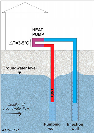
Figure 1.
The basic concept of an open-loop system.
An evaluation of the impact of shallow geothermal systems on the subsurface is necessary, due to the rapid increase in the number of installed open-loop systems in recent years [3,16,17,18,19,20,21,22]. Analytical solutions of flow and heat transfer equations are easy to use and therefore used in supporting open-loop system licensing procedures (e.g., in Guidelines for the use of groundwater heat pump systems in the state of Baden-Wuerttemberg, Germany [23]). Pophilat et al. [24] performed a comparison between three 2D analytical methods (radial, linear-advective and planar-advective heat transport model) and a 3D numerical method to specify the range of applicability of each analytical solution under different hydraulic conditions, to support integrated spatial planning in cities. They pointed out that the results are not intended to replace numerical simulations but could be a complementary tool to improve the groundwater management.
Numerical models at the urban scale that simulate the propagation of thermal plumes for investigated groundwater bodies are becoming increasingly used as a powerful decision-support tool for the management of shallow geothermal resources [17,18,22,25,26,27,28,29,30]. Thermal interference between open-loop systems has been analysed in the Po-Venice Plain region (IT), where a low hydraulic gradient and a lack of available space in densely populated historic urban areas make it difficult to install these systems [20]. Studies have also been made for urban areas with a high density of open-loop systems and a high hydraulic transmissivity, such as Basel (CH) or Zaragoza (ES) [22,26]. Additionally, Mueller et al. [22] assessed the thermal condition in Basel (CH) and proposed how this knowledge could be incorporated into urban planning. They found that elevated subsurface temperatures are mainly the result of anthropogenic activities, such as the sealing of surfaces, thermal groundwater use and the construction of deep buildings reaching the groundwater level. They suggested that monitoring and modelling tools should be integrated into the thermal management of urban groundwater bodies to ensure sustainability. On the other hand, Garcia-Gil et al. [28] analysed positive feedback from thermal interference between two open-loop systems (i.e., nesting system). The hot thermal plume generated by an upgradient cooling system had a positive effect on a downgradient heating system, which absorbs the heat from the thermal plume to satisfy its heating needs. Such a practice can only be used under controlled conditions, where the hydrogeological and thermal conditions are well known.
Piga et al. [31] have performed a sensitivity analysis with 3D numerical simulations on a representative model to assess the changes of dimensions of thermal plumes resulting from variations in hydrodynamic and thermal properties of the subsurface. Their results show the strong influence of groundwater flow velocity on the plume size and, for the long-term evolution of the plume, the influence of the ground thermal properties.
The aim of this study was to evaluate the impact of selected open-loop systems on the subsurface in the city centre of the City Municipality of Murska Sobota, NE Slovenia. The spatial density of installed open-loop systems in this area is increasing, and consequently also the risk of mutual interference between the systems which can lead to unsustainable use of geothermal potential. Based on the established monitoring network, fieldwork and known hydrogeological and thermal conditions in the area, we have developed a 3D numerical groundwater flow and heat transfer model to simulate thermal plumes and to provide information on the potential for new geothermal systems.
2. The Study Area
The study area is located in NE Slovenia, in the city centre of Murska Sobota (Figure 2). The City Municipality of Murska Sobota covers an area of 64 km2 and has 18,651 inhabitants. It is a flat area with an altitude ranging from 176 to 218 m a.s.l. and characterized by a continental climate. During the period 1961–2022, the average heating season duration was 240 days and average heating and cooling degree days were estimated to 3295 K/day and 38 K/day, respectively [32].
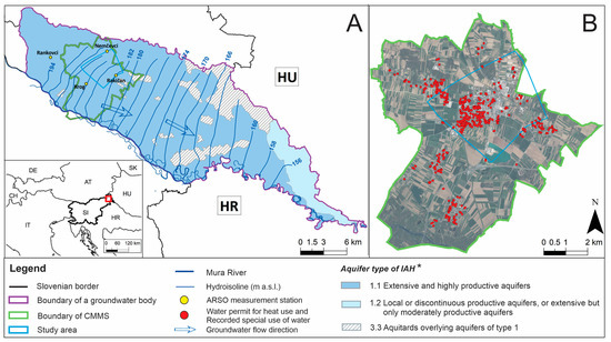
Figure 2.
(A) The location of the study area within Slovenia is marked with a red square, together with the basic hydrogeological map (* after [33]), on which the boundary of the City Municipality of Murska Sobota is marked with a green line. (B) Locations of existing water permits for heat use are marked with red circles [34,35]. The study area is marked with a blue line (source: [36]).
The use of low-temperature geothermal potential for heating with open-loop systems has increased in this area since 2014, and by 2022, 441 water permits and 216 permits for recorded special use of water had been granted (Figure 2B) [34,35]. The geometric mean of pumping rates in these geothermal systems was 1.1 L/s, with a minimum pumping rate of 0.5 L/s and a maximum pumping rate of 16 L/s. The maximum annual allowed groundwater withdrawal of all open-loop systems in total is around 4,900,000 m3 [34]. The high density of open-loop systems in this area is related to the presence of a highly productive, unconfined intergranular aquifer with an annual average groundwater temperature of 12 °C and a groundwater level averaging 3 m below the surface [37]. The general direction of the groundwater flow is from northwest to southeast (Figure 2A). The hydraulic conductivity of the aquifer ranges from 1 × 10⁻³ ms−1 to 5 × 10⁻³ ms−1 [37,38]. Groundwater in this area is mainly recharged by precipitation and partially by inflows from NW and from the hilly hinterland of Goričko on the northern edge of the Mura field [39].
The study area is part of the Mura field that is located on the western edge of the Pannonian Basin [40] and is filled with Quaternary, Pleistocene and Holocene sandy gravel sediments from the Mura River and its tributaries [41]. The Quaternary deposits are between 2 and 25 m thick, and their thickness gradually decreases towards the north-western part of the field. In the study area, Quaternary deposits are between 10 and 20 m thick and covered with a 0.3 to 4 m thick layer of fine-grained sediments from floodplains (sandy loam, sandy or silty clay) [41,42]. The base of the Quaternary sediments consists of Pliocene siltstones and sands, marls with sandstone and marly clays. The surface of the base dips in a southeasterly direction. In the northwestern part of the study area, the base is around 9 m below the surface, while in the southeastern part, it deepens to a depth of 18 m [41,42].
3. Materials and Methods
3.1. Monitoring Network
Groundwater level and temperature data were collected from the 15 wells, 7 pumping and 8 injection wells. The monitoring network was established on 15 December 2019 and is still operating. The recording interval was set to 15 min. In February 2021, we rearranged the monitoring network by moving the pressure and temperature sensors from 6 injection wells to pumping wells (Figure 3 and Figure 4). Additionally, in June 2021, we added 3 sensors in the pumping wells, where no impact from open-loop systems is anticipated.
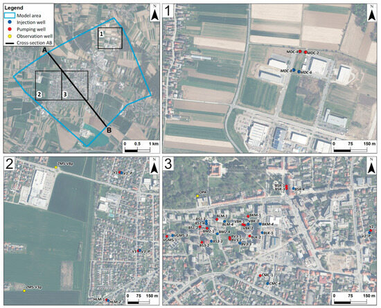
Figure 3.
Locations of the observation, pumping and injection wells included in the monitoring network, and the position of the cross-section is presented in Figure 5 (source: [36]).
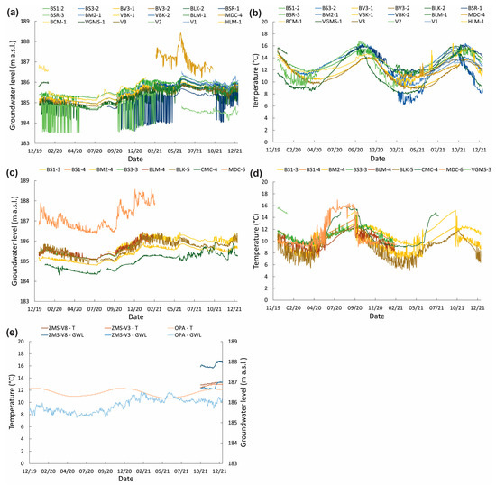
Figure 4.
Groundwater level and temperature measurements in pumping (a,b), injection (c,d) and observation wells (e).
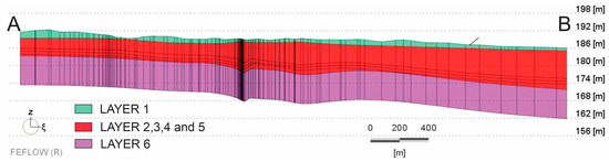
Figure 5.
Lithological cross-section A–B from northwest to southeast of the study area. The location of the profile is shown in Figure 3.
With this monitoring network, we have covered 16 water permits out of 388 permits (Figure 2B) issued in our study area inside the Municipality of Murska Sobota. If the installed capacity of groundwater heat pumps does not exceed 30 kW, owners are not obliged to have a system monitoring. Therefore, due to the fact that most of the small systems (<30 kW) are not monitored, we did not have the necessary data to include them in our numerical model. Nevertheless, we considered all larger systems in the city centre (>30 kW) and also set up monitoring for three smaller systems. The latter have similar annual pumping rates that the open-loop systems not included (the median of their allowed maximum pumping rate is 0.9 L/s), so we were able to analyse their extent and define whether there could be any other thermal impacts on the simulated thermal plumes.
The fluctuation of groundwater level and temperature in monitored wells are shown in Figure 4. During the monitored period, a positive trend in groundwater levels can be observed. This is consistent with groundwater levels recorded at national measurement stations in the vicinity, where a positive trend has also been evident over the last 30 years, which is related to increased precipitation in the area [32].
Due to the shallow groundwater level in the unconfined aquifer, a rapid response of groundwater level to precipitation is observed (Figure 4). Large short-term groundwater level and temperature fluctuations (Figure 4) indicate the operation period of the open-loop systems. Daily pumping data was obtained from the local operator of the open-loop systems.
3.2. FEM Numerical Model
Modelling was performed with the use of the FEM (Finite Element Model) numerical code FEFLOW 8.0 [43]. A steady-state groundwater flow and thermal simulations were performed to define the initial conditions with fixed boundary conditions and material properties. The aquifer was simulated as unconfined with an upper phreatic layer, which means that the elements in this layer can become dry or partially saturated [43]. The Darcy equation was used for the other layers. The resulting hydraulic head and temperature distribution formed the basis for further transient simulations of groundwater level fluctuations and temperature distributions.
3.3. Model Setup
A total of 6 layers and 7 slices were integrated into the model to adequately include the measurements of groundwater level and temperature. While the layers define the extent of each prism and contain the material properties, the slices define the upper and lower boundaries of each prism and are associated with the nodes of the prismatic elements to which the computational results refer [43]. The assigned material properties for the layers are presented in Table 1, and the cross-section through the study area is shown in Figure 5. The lowest layer represents the base of the alluvial aquifer and was uniformly set to 10 m thickness (slices 6 and 7). Slice 6 was determined based on the lithological profiles and borehole reports of the 99 wells [38,44,45,46,47,48,49,50,51]. Layers 2, 3, 4 and 5 represent the alluvial aquifer and have the same properties.
The top of layer 2 (slice 2) corresponds to the boundary between clayey/silty and sandy/gravely sediments, observed in the lithological profiles of 96 wells. Slice 3 represents the depth of temperature sensors in pumping wells, slice 4 represents the top of the filters in wells, and slice 5 represents the depth of temperature sensors in injection wells. The vertical division of the alluvial aquifer into layers was performed to increase the modelling resolution of the heat exchange around the open-loop systems and in the wells’ filter zones. Layer 1 represents more silty sands and gravel sediments covering the alluvial aquifer, which partially slow the vertical flow of rainwater through the cover [38]. In some areas, the layer is only a few decimetres thick and therefore provides low natural protection for the aquifer. The topography of the model (slice 1) was derived from a digital elevation model with a 20 m resolution [52]. The elevation decreases from northwest to southeast and ranges from 193.4 m a.s.l. in the northwest to 183.7 m a.s.l. in the southeast.

Table 1.
Hydraulic and thermal material properties are assigned to the model layer as a uniform value, together with the layer thickness.
Table 1.
Hydraulic and thermal material properties are assigned to the model layer as a uniform value, together with the layer thickness.
| Layer | |||
|---|---|---|---|
| 1 | 2, 3, 4 and 5 | 6 | |
| Layer thickness (m) | 0.1–12.5 | 4.8–18.5 | 10 |
| Material property | |||
| Hydraulic conductivity (ms−1) | 2.8 × 10⁻⁵ [a] | 1.0 × 10⁻³ [b] | 1 × 10⁻⁷ [c] |
| Effective porosity (Fluid) (-) | 0.4 [c] | 0.15 [a] | 0.5 [c] |
| Total porosity (Heat) (-) [d] | 0.5 | 0.25 | 0.6 |
| Volumetric heat capacity of solid material (MJm−3K−1) [d] | 1.5 | 2.5 | 2.5 |
| Thermal conductivity of solid material (Wm−1K−1) [d] | 1.5 | 3.0 | 3.7 |
[a] field measurements [38,44,45]; [b] borehole reports [46,47,48,49,50,51]; [c] borehole reports [53,54]; [d] laboratory measurements.
3.4. Mesh Geometry
The finite element mesh covers an area of 5470 m × 5104 m and includes the observed open-loop systems and an additional area created with a buffer distance of 500 m. We used this buffer zone to reduce the influence of boundary conditions on observed open-loop systems. The mesh consists of 68,706 elements and 40,397 nodes. The resulting volume of the 3D model is 3.19 × 10⁸ m3, with an overall depth of 35.5 m.
The discretisation of the study area was performed with a triangular algorithm. The refinement of the mesh was performed in the proximity of the pumping and injection wells. The maximum side length for the elements directly at the refined point was set to 3 m, while the smoothness of the transition from the fine elements to the coarser elements was set to 2. To reduce truncation errors during the numerical computation and to improve the convergence behaviour of the model, we smoothed the finite-element mesh three times. We manage to smoothen the maximum interior angle of triangles from 77° to 73°. The well positions were not part of the smoothing to avoid shifting of their positions.
3.5. Boundary Conditions
The Dirichlet boundary condition (BC) at the northwestern and southeastern boundaries was set parallel to the average piezometric lines of the Rankovci, Krog, Nemčavci and Rakičan measurement stations and perpendicular to the groundwater flow (yellow points in Figure 2A) [37]. For initial conditions, we set the upstream groundwater level at 187.36 m a.s.l. and downstream at 182.46 m a.s.l. For the transient simulation, we set Dirichlet BC using daily groundwater level data from the Nemčevci measurement station in the northwest and the Rakičan measurement station in the southeast. Eastern and western boundaries were set as no-flow boundaries.
Soil temperature measurements at 50 cm depth at the Rakičan measurement station were used as a temperature BC at the top of the model [32]. The thermal balance of the aquifer under steady-state conditions was reproduced by applying the undisturbed soil temperature of 12.5 °C (average soil temperature in 2020) on the top of the model domain. On the bottom of the model, a constant geothermal heat flux of 0.145 Wm−2 was set as Neumann BC [55]. The average depth of the aquifer is only 10 m, and since thermal conditions in the aquifer are mainly influenced by the ambient or surface temperature, we did not define detailed vertical temperature-depth boundary conditions at the lateral boundaries of the model. We assigned time-varying temperature BC at the top of the model for areas without buildings. To account for the thermal input from the buildings [3], we assigned a constant temperature of 15 °C to the areas with buildings. Due to the scarcity of data about temperature conditions and the depth of building basements, it is a roughly estimated BC.
On the top layer, we have included polygons with different land use (Figure 6), to distinguish between urban and agricultural areas. For these areas, different infiltration values were calculated using daily precipitation and evapotranspiration data from the Rakičan measurement station [32]. Additionally, we reduced the obtained infiltration values based on the runoff coefficient for urban (0.2) and agricultural (0.5) areas [56].
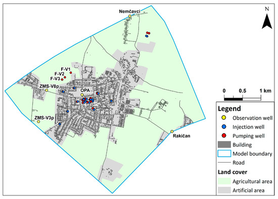
Figure 6.
Study area with used observation, injection and pumping wells, buildings, roads, and land cover data. Observation and pumping wells for drinking water supply are labelled, other wells are labelled in Figure 3.
The pumping and injection rates were assigned to specific depths for individual wells, corresponding to their filter depths, through the multilayer wells BC (Table 2). We included also the pumping rates of the three wells, which are used for drinking water supply (F-V1, F-V2, F-V3 in Table 2). For 16 open-loop systems, we assigned the reported daily pumping (P) and injection (I) rates. Data on the P/I rates were available for the entire open-loop system, but not for individual wells within the system. Therefore, we considered one well doublet for each open-loop system, even if there are multiple doublets used (Table A1 in Appendix A). For open-loop system 6 (Table 2), we assigned P/I rates for 2 of 4 doublets. The average distance between pumping wells in each system is approximately 10 m. These wells do not operate simultaneously, but alternate based on predefined settings provided by the local operator. Consequently, representing these wells as a single well in the model does not compromise the model’s reliability significantly.
Table 2.
Open-loop doublets and drinking water supply wells used in the numerical simulation. Pumping (P) and injection (I) rates are presented for the time period of 746 days, excluding days without P/I.
The temperature difference between pumping and injecting water was set as a constant value of 3 K. Assuming this temperature differential, the injection temperature depends on the unknown extraction temperature, which cannot be determined by a statically given boundary condition but must be calculated dynamically during the simulation. Therefore, we used the OpenLoop plug-in, which is integrated in the FEFLOW 8.0 software [57].
Locations, well depths, filter depths, pumping and injection rates included in the model are presented in Table 2.
3.6. Calibration and Validation
The model is based on data from 15 December 2019 to 31 December 2021. Continuous groundwater level and temperature data from 29 locations, ranging from 366 to 745 days (year 2021) were used to calibrate the groundwater flow and heat models. The validation of the models was based on a simulation time of 0 to 365 days (year 2020) at 19 locations, which were also used in the calibration procedure. The second year of monitoring data obtained was used for calibration, as we had more data than the first year, which was then used for the validation.
Groundwater level and temperature data were extracted from the model 5 m north of the actual wells, except for observation wells. We moved the observation points because of large fluctuations in the measured data during system operation due to pressure losses in the pumping wells or artificially elevated groundwater levels in the injection wells. To exclude these influences from interfering with the calibration procedure, we used the maximum and minimum moving average for 3 to 6 days. The same was completed for the measured temperature data, as these are influenced by the operating pumps in the wells.
The hydraulic and thermal parameters were calibrated using the PEST algorithm for automatic parameter estimation implemented in FEFLOW with the FePEST utility [58]. The calibration of transient numerical models requires a high effort in terms of the number of runs and computational time. Since the number of simulations required for the automatic calibration algorithm is proportional to the number of variable parameters identified, the parameter space was optimised to reduce the computation time [58]. Only the layers representing the aquifer (layers 2, 3, 4 and 5) were selected for spatial calibration of the parameters. The parameters of the other layers remained zonally constant, with the initial parameters listed in Table 1.
To further optimise the computational time for calibration, the number of calibrated parameters was reduced to hydraulic conductivity for the flow model and total porosity and dispersivity for the heat transfer model. The parameters were chosen based on the first iteration, where the influence of the initial parameter values on the observations is expressed in a Jacobian matrix. Table 3 presents the calibrated parameters, their initial values, and upper and lower limits. The lower and upper limits of hydraulic conductivity were based on reported values [46,47,48,49,50,51], and for the thermal parameters laboratory measurements were used which formed the basis for the simulated spatial variability. Thermal dispersivity (longitudinal, transverse) in heterogeneous aquifers has a greater impact on the distribution of thermal plumes because it is related to the advective component of the heat flow [59,60]. In the study area, no field data are available for the estimation of dispersivity. Longitudinal thermal dispersivity in sediments can range from 0 to 100 m [59]. Based on previous studies of similar intergranular aquifers [60], we decided to define the range of thermal longitudinal dispersivity between 4 and 30 m.
Table 3.
Hydraulic and thermal parameters calibrated in the model.
The deviation between the measured and simulated groundwater levels and temperatures was evaluated by comparing their daily root mean square error (RMSE).
4. Results and Discussion
4.1. Calibration
The composite sensitivity values determined for the hydraulic and thermal parameters (Figure 7) are derived from the Jacobian matrix and indicate the extent to which all simulations are sensitive to an individual parameter [61]. The calibrated values for hydraulic conductivity are on average 2.2 × 10⁻³ ms−1. To minimise the error between the measured and simulated groundwater temperature for the heat transfer model, the total porosity and thermal dispersivity were selected for calibration, according to their higher composite sensitivity (Figure 7). The calibrated total porosity in the study area averages 0.35. The calibrated longitudinal dispersivity is on average 13.8 m. Transverse dispersivity is assumed to be 10 times lower.
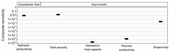
Figure 7.
Composite sensitivity of hydraulic and thermal parameters derived from the Jacobian matrix.
The calibration results are shown in Figure 8 by plotting the average daily values of measured and simulated groundwater levels and temperatures. The daily variations of the measured and simulated data for each location, with their RMSE values, are in Appendix A (Figure A1, Figure A2 and Figure A5).
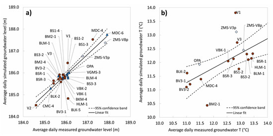
Figure 8.
Scatter plot of average measured and simulated (a) groundwater levels (29 locations) and (b) groundwater temperature (18 locations) after calibration. Circles denote pumping, triangles are injection and diamonds are observation wells.
The average RMSE between simulated and measured groundwater level data during the dynamic simulation is lowest for the observation wells (RMSE = 0.09 m) (Figure A5). The error remains constant during almost the entire simulation period. It increases by 0.1 m in the last 80 days of calibration when new data from the edges of our model are added. For the pumping wells, the average error during calibration is 0.19 m and for the injection wells, it is 0.16 m. The RMSE values show that the BC and the parameters in the model are adequately defined when compared to the calibration results of models of similar aquifers, like Basel or Milano (RMSE is on average 0.3 m) [22,27].
The average RMSE between simulated and measured temperature data during the dynamic simulation is 0.76 °C for the observation wells. It shows clear seasonal variations, with the error ranging from 0–1.5 °C (Figure A5). For the pumping wells, the average RMSE is 0.95 °C and is almost constant during the simulation period. On average, the error in the temperature data in the wells is higher during the summer months when the open-loop systems are not in operation. The simulated temperatures are lower than the measured ones, which is probably due to locally underestimated thermal sources at the surface (sewage, plumbing, buildings with more than one basement and roads). The RMSE between simulated and observed groundwater temperatures for the aquifer beneath Milano (IT) [27] and Basel (CH) [22] showed errors in a similar range (0.3–1.2 °C) as our results. As possible main causes for the errors, they pointed out additional thermal sources at the subsurface, misrepresented phasing of the temperature signal due to thermal parameters and the warming trend of the subsurface, which were not considered in the simulations.
4.2. Validation
The simulated groundwater level and temperature regime were validated by comparing the model results with data from 20 locations, for a simulation period of 0 to 365 days (Table 4, Figure A3, Figure A4 and Figure A6 in Appendix A). The comparison between the average measured and simulated data is shown on a scatter plot (Figure 9).
Table 4.
Comparison of average measured and simulated groundwater levels and temperature, together with their RMSE (validation period). P—pumping well, I—injection well, O—observation well.
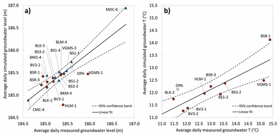
Figure 9.
Scatter plot of average measured and simulated (a) groundwater levels (20 locations) and (b) groundwater temperature (10 locations) in the validation period. Circles mark pumping wells, triangle mark injection wells and diamonds mark observation wells.
The results show that the simulated groundwater levels differ from the observed by 0.2 m on average. The deviation could be caused because of simplifying the operation of open-loop systems, which use a total pumping rate that is not separated into individual well doublets. On the other hand, the simulated groundwater temperatures are on average 1 K lower than the measured values (Figure 9b). Even higher differences can be seen for number 30, which is related to the short observation period for this well, which was not included in the calibration. The underestimation of the simulated temperature data is especially visible in the summer months when the systems are not operating (Figure A4 in Appendix A). As mentioned, this might be related to some additional thermal sources on the surface, such as heat input from buildings and roads and underground infrastructure. Their influence is difficult to assess, due to the lack of monitoring data in the unsaturated zone. Similar deviations between simulated and measured groundwater temperatures have been observed in the unconfined aquifer of Basel and Locarno City (Switzerland) and Milan City (Italy) [22,27,62]. Their results suggest that the heat inflow in the summer months is underestimated (difference around 2 K or even higher), which could be the consequence of an underestimated initial temperature in specific locations, an underestimated or neglected thermal energy released by specific sources in the subsurface, and/or incorrectly estimated parameters that could prevent heat accumulation in the aquifer. Due to the lack of temperature measurements, they did not investigate further which heat source or parameter was misestimated.
4.3. Simulated Thermal Plumes Downgradient from Injection Wells
In Figure 10 we see that the simulated thermal plumes of wells V2 and VGMS-3 have a maximum dimension of 2 m to 20 m, respectively. We believe that the pumping rates of wells V2 and VGMS-3 are similar for most open-loop systems (small individual houses) that were not included in the numerical model due to no monitoring data. Based on these dimensions of the thermal plumes (wells V2 and VGMS-3) we believe that there were no additional hydraulic or thermal influences on the simulated thermal plumes of the open-loop systems that were included in the numerical simulation.
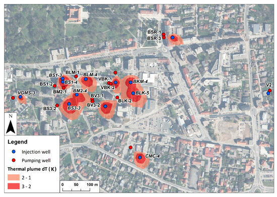
Figure 10.
Simulated thermal plumes from the injection wells in mid-April 2020, when their dimensions are the greatest and groundwater temperatures the lowest.
The transient numerical simulation of the impact of observed open-loop systems in the city centre has shown that the thermal plumes propagate downgradient from the injection wells between 50 m and 100 m, and their width is at most 120 m. Their dimensions depend on the pumping rate and the proximity of the other injection wells, which can lead to a merging of two plumes and consequently cause larger groundwater temperature changes. In Figure 10, we see the maximum dimensions of the thermal plumes that occur in mid-April, when groundwater temperatures reach their lowest values. Groundwater temperatures at the pumping wells are restored during the summer when the systems are not in operation, so the thermal plumes do not extend throughout the year.
At two locations (BLK-5 and MDC-6 (Figure A7 in Appendix A)) the thermal plumes are not fully restored until the beginning of the new heating season. This is because these open-loop systems are also in operation during the summer months to meet the demand for domestic hot water.
Migrating thermal plumes in the city centre during the heating period generally do not affect the efficiency of other open-loop systems. The only locations where simulated groundwater temperatures are affected by nearby cold thermal plumes are locations BM2-1, BV3-1, BV3-2, and VBK-2 (Figure 10). For location BM2-1, we do not have real data on groundwater temperatures because monitoring in the well was not possible due to lack of space in the pumping well BM2-1. Therefore, we cannot confirm our simulated results. For the location with pumping wells BV3-1 and BV3-2, the measured groundwater temperature is on average 1 K lower than in the pumping wells located upgradient (BS1-2, BS3-2) (Figure 4b). This can also be seen in Figure 10, where cold thermal plumes from wells BM2-4 and BS3-3 reach the pumping wells, and change the groundwater temperature by 1 to 2 °C. The extent of this cold thermal plume shown in Figure 10 (BM2-4, BS3-3) is highest at the end of the heating season because a larger volume of cold groundwater is injected and the injection wells are too close to each other so that they begin to interfere with each other. In other months, the extent of the cold thermal plume is not so great and therefore does not influence the groundwater temperature in the downgradient pumping wells BV3-1 and BV3-2. For location VBK-2 (Figure 10), the simulated lower groundwater temperature in the well is not the result of an upgradient cold thermal plume but is related to a nearby injection well of the same open-loop system, that was drilled too close, resulting in a thermal breakthrough in pumping well VBK-2. The actual measured groundwater temperature is also quite low (Figure 4b). Besides the thermal breakthrough, the improper construction of well VBK-2 was probably also the reason that cold rainwater could infiltrate into the aquifer and additionally lower the groundwater temperature.
5. Conclusions
We developed a complex numerical model that provides insights into the hydraulic and thermal conditions of the shallow alluvial aquifer, as well as the possible interactions between the observed open-loop systems and their long-term efficiency. The established monitoring network at the city scale in NE Slovenia was the basis for the development of the groundwater flow and heat transport model. The thermal plumes caused by open-loop systems need to be well predicted and continuously monitored, especially in the shallow aquifers of densely populated areas, like in our study area in the City Municipality of Murska Sobota. This is important not only to ensure long-term sustainable use of the systems but also to avoid negative impacts on the efficiency of neighbouring geothermal systems.
The results represent simulated groundwater flow and thermal regime from December 2019 to the end of December 2021. The sensitivity analysis showed the highest composite sensitivity values for hydraulic conductivity, porosity and dispersivity parameters, which were further calibrated with FePEST to minimize the error between groundwater level and temperature. The RMSE for the simulated groundwater level ranges from 0.09 to 0.19 m and from 0.14 to 0.26 m for the calibration (29 wells) and validation (20 wells) datasets, respectively. For the groundwater temperature data, the RMSE values range between 0.76 and 0.95 °C and between 0.85 and 1.01 °C for calibration (18 wells) and validation (10 wells) datasets, respectively.
The results of the groundwater flow model correspond well with the measured average groundwater levels. On the other hand, the thermal model shows higher deviations from the measured data, especially in the summer months when the simulated groundwater temperatures do not exceed 14.3 °C, while the measured temperatures reached even 15.4 °C. These deviations could be related to the effects of local thermal sources on the surface (e.g., sewage pipes, plumbing, buildings with more than one basement and roads), which were not considered in our model. The results are comparable to other studies on similar aquifers under larger cities in Europe [22,27,62] mentioned in the discussion, where the deviation between measured and simulated groundwater temperatures also reached 2 K. As thermal dispersivity in heterogeneous aquifers can have a greater impact on heat transport in the vicinity of open-loop systems a push-pull test could be performed in the field in the future to confirm the accuracy and currently defined ranges in the heat transfer model [59,63].
The simulated thermal plumes caused by the existing open-loop systems in the city centre of the Murska Sobota generally show no mutual interference between the systems that could significantly affect their efficiency. The transient simulation showed that the thermal plumes do not propagate throughout the year, which indicates that groundwater temperatures recover in summer when the systems are not in operation.
Appropriate management concepts are required for the future sustainable development of subsurface resources. Due to the high density of existing systems in the studied area, it is recommended that simulations of the thermal plumes of new geothermal systems are conducted before installing them, so they will not affect the efficiency of the existing systems.
Author Contributions
Conceptualization, S.A., M.J. and M.B.; data curation, S.A.; formal analysis, S.A. and M.J.; funding acquisition, M.J.; investigation, S.A.; methodology, S.A. and M.J.; project administration, M.J.; supervision, M.J. and M.B.; validation, S.A. and M.J.; visualization, S.A.; writing—original draft, S.A.; writing—review and editing, M.J. and M.B. All authors have read and agreed to the published version of the manuscript.
Funding
The research was funded by the Slovenian Research and Innovation Agency (ARIS) through research program P1-0020 Groundwater and Geochemistry in the frame of the Young Researchers programme, and by the UNESCO IGCP Project 684—The Water-Energy-Food and Groundwater Sustainability Nexus. The equipment for the monitoring network was co-financed by the Republic of Slovenia, Ministry of Education, Science and Sport and the European Union from the European Regional Development Fund through the project “Development of research infrastructure for the international competitiveness of the Slovenian RRI space—RI-SI-EPOS.
Institutional Review Board Statement
Not applicable.
Informed Consent Statement
Not applicable.
Data Availability Statement
Not applicable.
Acknowledgments
The authors wish to thank Uroš Klemenčič, from Ouček d.o.o. company, for the help with the establishment and maintenance of the monitoring network.
Conflicts of Interest
The authors declare no conflict of interest.
Appendix A
Table A1.
Number of doublets for an individual open-loop system.
Table A1.
Number of doublets for an individual open-loop system.
| Open-Loop System | Well Name with Assigned P/I Rate | Number of Pumping Wells | Number of Injection Wells |
|---|---|---|---|
| 1 | BS1-2/19 | 2 | 2 |
| BS1-3/19 | |||
| 2 | BM2-1/19 | 2 | 2 |
| BM2-4/19 | |||
| 3 | BS3-2/19 | 2 | 2 |
| BS3-3/19 | |||
| 4 | BLM-1/19 | 2 | 2 |
| BLM-4/19 | |||
| 5 | BLK-2/16 | 3 | 3 |
| BLK-5/16 | |||
| 6 | MDC-2/18 | 4 | 4 |
| MDC-6/18 | |||
| MDC-4/18 | |||
| MDC-8/18 | |||
| 7 | CMC-1/17 | 2 | 2 |
| CMC-4/17 | |||
| 8 | BKM-1/19 | 2 | 2 |
| BKM-4/19 | |||
| 9 | V1 | 1 | 1 |
| V1_P | |||
| 10 | V2 | 1 | 1 |
| V2_P | |||
| 11 | V3 | 1 | 1 |
| V3_P | |||
| 12 | VBK-1/16 | 2 | 2 |
| VBK-3/16 | |||
| 13 | BV3-1/19 | 2 | 2 |
| BV3-3/19 | |||
| 14 | BSR-1/19 | 3 | 1 |
| BSR-4/19 | |||
| 15 | VGMS-1/13 | 2 | 2 |
| VGMS-3/13 | |||
| 16 | HLM-1/14 | 1 | 1 |
| HLM-2/14 | |||
| Drinking water supply | F-V1 | 3 | / |
| F-V2 | |||
| F-V3 |
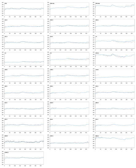
Figure A1.
Daily measured (black line) and simulated (dashed blue line) groundwater levels for 3 observed, 15 pumping and 10 injection wells after calibration.
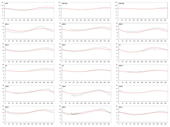
Figure A2.
Daily measured (black line) and simulated (dashed red line) groundwater temperatures for 3 observed and 15 pumping wells after model calibration.
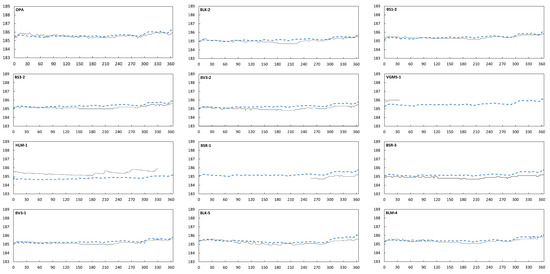
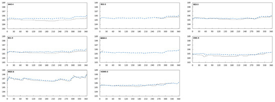
Figure A3.
Daily measured (black line) and simulated (dashed blue line) groundwater levels for 1 observed, 9 pumping and 10 injection wells in the validation process.
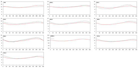
Figure A4.
Daily measured (black line) and simulated (dashed red line) groundwater temperatures for 1 observed and 9 pumping wells in the validation process.
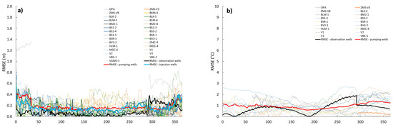
Figure A5.
RMSE between simulated and observed groundwater level (a) and temperature (b) after calibration.
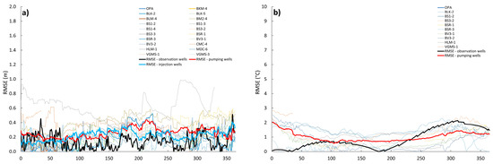
Figure A6.
RMSE between simulated and observed groundwater level (a) and temperature (b) in the validation process.
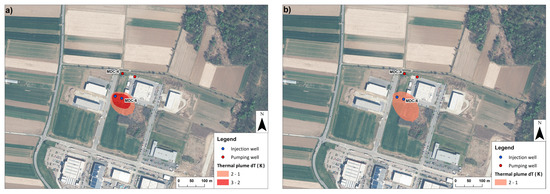
Figure A7.
Simulated thermal plume from injection wells MDC-6 and MDC-8 in the middle of April 2020, when their dimensions are the greatest (a) and at the end of September 2020, when their dimensions are the lowest (b).
References
- European Council. Communication on REPowerEU: Joint European Action for More Affordable, Secure and Sustainable Energy, COM, 108 Final; European Council: Brussels, Belgium, 2022. [Google Scholar]
- Ministry of Infrastructure. Integrated National Energy and Climate Plan of the Republic of Slovenia; Ministry of Infrastructure: Ljubljana, Slovenia, 2020; 233p.
- Epting, J.; Handel, F.; Huggenberger, P. Thermal management of an unconsolidated shallow urban groundwater body. Hydrol. Earth Syst. Sci. 2013, 17, 1851–1869. [Google Scholar] [CrossRef]
- Garcia-Gil, A.; Schneider, E.; Moreno, M.; Santamarta, J. Shallow Geothermal Energy: Theory and Application; Springer: Cham, Switzerland, 2022. [Google Scholar]
- Banks, D. An Introduction to Thermogeology: Ground Source Heating and Cooling, 2nd ed.; Wiley-Blackwell: Hoboken, NJ, USA, 2012. [Google Scholar]
- EGEC. Geothermal Market Report 2020; European Geothermal Energy Council: Brussels, Belgium, 2021. [Google Scholar]
- Lund, J.W. Ground-Source (Geothermal) Heat Pumps. In Course on “Heating with Geothermal Energy: Conventional and New Schemes”; Lienau, P.J., Ed.; WGC2000 Short Courses: Kazuno, Japan, 2000; pp. 209–236. Available online: https://www.geothermal-energy.org/pdf/IGAstandard/ISS/2001Romania/lund_hp.pdf (accessed on 5 June 2022).
- De Moel, M.; Bach, P.M.; Bouazza, A.; Singh, R.M.; Sun, J.O. Technological advances and applications of geothermal energy pile foundations and their feasibility in Australia. Renew. Sustain. Energy Rev. 2010, 14, 2683–2696. [Google Scholar] [CrossRef]
- Chiasson, A.D. Geothermal Heat Pump and Heat Engine Systems—Theory and Practice; Wiley, Department of Mechanical and Aerospace Engineering, University of Dayton: Dayton, OH, USA, 2016. [Google Scholar]
- Kłonowski, M.; Kozdrój, W.; Götzl, G.; Heiermann, M. Summary Report on Existing Energy Planning Strategies in the EU Considering the Use of Shallow Geothermal Energy; Interreg Central Europe: Wien, Austria, 2018. [Google Scholar]
- Banks, D. The application of analytical solutions to the thermal plume from a well doublet ground source heating or cooling scheme. Q. J. Eng. Geol. Hydrogeol. 2011, 44, 191–197. [Google Scholar] [CrossRef]
- Molina-Giraldo, N.; Bayer, P.; Blum, P. Evaluating the influence of thermal dispersion on temperature plumes from geothermal systems using analytical solutions. Int. J. Therm. Sci. 2011, 50, 1223–1231. [Google Scholar] [CrossRef]
- Wu, Q.; Tu, K.; Sun, H.; Chen, C. Investigation on the sustainability and efficiency of single-well circulation (SWC) groundwater heat pump systems. Renew. Energy 2019, 130, 656–666. [Google Scholar] [CrossRef]
- Al-Khoury, R. Computational Modeling of Shallow Geothermal Systems; Taylor & Francis Group: Abingdon, UK, 2012; Volume 4. [Google Scholar]
- Sass, I.; Brehm, D.; Coldewey, W.G.; Dietrich, J.; Klein, R.; Kellner, T.; Kirschbaum, B.; Lehr, C.; Marek, A.; Mielke, P.; et al. Shallow Geothermal Systems—Recommendations on Design, Construction, Operation and Monitoring; Wilhelm Ernst & Sohn: Berlin, Germany, 2016. [Google Scholar]
- Epting, J.; Huggenberger, P. Unraveling the heat island effect observed in urban groundwater bodies—Definition of a potential natural state. J. Hydrol. 2013, 501, 193–204. [Google Scholar] [CrossRef]
- Muela Maya, S.; García-Gil, A.; Garrido Schneider, E.; Mejías Moreno, M.; Epting, J.; Vázquez-Suñé, E.; Marazuela, M.Á.; Sánchez-Navarro, J.Á. An upscaling procedure for the optimal implementation of open-loop geothermal energy systems into hydrogeological models. J. Hydrol. 2018, 563, 155–166. [Google Scholar] [CrossRef]
- Attard, G.; Bayer, P.; Rossier, Y.; Blum, P.; Eisenlohr, L. A novel concept for managing thermal interference between geothermal systems in cities. Renew. Energy 2020, 145, 11. [Google Scholar] [CrossRef]
- Di Dato, M.; D’Angelo, C.; Casasso, A.; Zarlenga, A. The impact of porous medium heterogeneity on the thermal feedback of open-loop shallow geothermal systems. J. Hydrol. 2022, 604, 127205. [Google Scholar] [CrossRef]
- Previati, A.; Crosta, G.B. Regional-scale assessment of the thermal potential in a shallow alluvial aquifer system in the Po plain (northern Italy). Geothermics 2021, 90, 101999. [Google Scholar] [CrossRef]
- Lo Russo, S.; Taddia, G.; Verda, V. Development of the thermally affected zone (TAZ) around a groundwater heat pump (GWHP) system: A sensitivity analysis. Geothermics 2012, 43, 66–74. [Google Scholar] [CrossRef]
- Mueller, M.H.; Huggenberger, P.; Epting, J. Combining monitoring and modelling tools as a basis for city-scale concepts for a sustainable thermal management of urban groundwater resources. Sci. Total Environ. 2018, 627, 1121–1136. [Google Scholar] [CrossRef]
- Baden Württemberg Umweltministerium. Leitfaden zur Nutzung von Erdwärme mit Grundwasserwärmepumpen; Baden Württemberg Umweltministerium: Stuttgart, Germany, 2009.
- Pophillat, W.; Attard, G.; Bayer, P.; Hecht-Méndez, J.; Blum, P. Analytical solutions for predicting thermal plumes of groundwater heat pump systems. Renew. Energy 2018, 147, 2696–2707. [Google Scholar] [CrossRef]
- Böttcher, F.; Casasso, A.; Götzl, G.; Zosseder, K. TAP—Thermal aquifer Potential: A quantitative method to assess the spatial potential for the thermal use of groundwater. Renew. Energy 2019, 142, 85–95. [Google Scholar] [CrossRef]
- Epting, J.; García-Gil, A.; Huggenberger, P.; Vázquez-Suñe, E.; Mueller, M.H. Development of concepts for the management of thermal resources in urban areas—Assessment of transferability from the Basel (Switzerland) and Zaragoza (Spain) case studies. J. Hydrol. 2017, 548, 697–715. [Google Scholar] [CrossRef]
- Previati, A.; Epting, J.; Crosta, G.B. The subsurface urban heat island in Milan (Italy)—A modeling approach covering present and future thermal effects on groundwater regimes. Sci. Total Environ. 2022, 810, 152119. [Google Scholar] [CrossRef]
- García-Gil, A.; Mejías Moreno, M.; Garrido Schneider, E.; Marazuela, M.Á.; Abesser, C.; Mateo Lázaro, J.; Sánchez Navarro, J.Á. Nested Shallow Geothermal Systems. Sustainability 2020, 12, 5152. [Google Scholar] [CrossRef]
- García-Gil, A.; Muela Maya, S.; Garrido Schneider, E.; Mejías Moreno, M.; Vázquez-Suñé, E.; Marazuela, M.Á.; Mateo Lázaro, J.; Sánchez-Navarro, J.Á. Sustainability indicator for the prevention of potential thermal interferences between groundwater heat pump systems in urban aquifers. Renew. Energy 2019, 134, 14–24. [Google Scholar] [CrossRef]
- Pophillat, W.; Bayer, P.; Teyssier, E.; Blum, P.; Attard, G. Impact of groundwater heat pump systems on subsurface temperature under variable advection, conduction and dispersion. Geothermics 2020, 83, 101721. [Google Scholar] [CrossRef]
- Piga, B.; Casasso, A.; Pace, F.; Godio, A.; Sethi, R. Thermal Impact Assessment of Groundwater Heat Pumps (GWHPs): Rigorous vs. Simplified Models. Energies 2017, 10, 1385. [Google Scholar] [CrossRef]
- ARSO. Meteo Archive. Available online: https://meteo.arso.gov.si/met/sl/archive/ (accessed on 5 June 2022).
- Struckmeier, W.; Margat, J.F. Hydrogeological Maps: A Guide and a Standard Legend; Heise: Hannover, Germany, 1995. [Google Scholar]
- DRSV. Water Permits for Heat Use. Available online: https://vode.dv.gov.si/vdvpogled/Poizvedba.jsp (accessed on 5 June 2022).
- Vodna Knjiga. Ministrstvo za Naravne Vire in Prostor, Direkcija Republike Slovenije za Vode. Available online: https://podatki.gov.si/dataset/vodna-knjiga?resource_id=b852ff63-f0a2-42b7-abad-6975f9a7378e (accessed on 1 August 2023).
- GURS. Digitalni Ortofoto Posnetki DOF50. 2019. Available online: https://podatki.gov.si/dataset/ortofoto (accessed on 12 March 2022).
- ARSO. Hydrological Data Archive. Available online: http://vode.arso.gov.si/hidarhiv/ (accessed on 2 June 2022).
- Brenčič, M.; Bole, Z. Hidrogeološki Elaborat za Potrebe Idejnega Projekta Izvenivojskega Križanja z Železnico v Murski Soboti na R2-441/1298 (Lendavska); Geološki zavod Slovenije: Ljubljana, Slovenia, 2000; p. 20. [Google Scholar]
- Koren, K.; Brenčič, M.; Lapanje, A. Hydrogeology of the transition area between Prekmursko polje and Goričko (NE Slovenia). Geologija 2015, 58, 175–182. [Google Scholar] [CrossRef]
- Novak, M.; Bavec, M.; Trajanova, M. Lithological map of Slovenia. In Geological atlas of Slovenia, 2nd ed.; Novak, M., Rman, N., Eds.; Geological Survey of Slovenia: Ljubljana, Slovenia, 2016. [Google Scholar]
- Pleničar, M. Tolmač za Lista Goričko Osnovne Geološke Karte SFRJ 1:100,000; Zvezni Geološki Zavod Beograd: Belgrade, Serbia, 1970; p. 39. [Google Scholar]
- Mioč, P.; Markovič, S. Osnovna Geološka Karta R Slovenije in R Hrvaške—List Čakovec 1:100,000; Institut za Geoloska Istrazivanja: Zagreb, Croatia, 1998. [Google Scholar]
- Diersch, H.-J. FEFLOW: Finite Element Modeling of Flow, Mass and Heat Transport in Porous and Fractured Media; Springer Science & Business Media: New York, NY, USA, 2014. [Google Scholar]
- Ratej, J.; Kranjc, T.; Narat, D.; Kocjančič, M.; Ivačič, B. Hidrogeološki Elaborat za Potrebe Izvedbe Trase Vzhodne Obvoznice Murska Sobota od km 3+520 do km 6+940; IRGO Consulting d.o.o.: Ljubljana, Slovenia, 2018; p. 50. [Google Scholar]
- Prestor, J.; Strojan, M. Hidrogeološko Poročilo o Vodnjaku V-INOKS Galvanika, Podjetja “Inoks”—Izpostava Murska Sobota; Geološki zavod Slovenije: Ljubljana, Slovenia, 2004; p. 9. [Google Scholar]
- Bokan, A. Hydrogeological Reports for Water Permit of Individual Open-Loop Systems; GEO-VRTINA d.o.o.: Murska Sobota, Slovenia, 2020. [Google Scholar]
- Bokan, A. Hydrogeological Reports for Water Permit of Individual Open-Loop Systems; GEO-VRTINA d.o.o.: Murska Sobota, Slovenia, 2019. [Google Scholar]
- Bokan, A. Hydrogeological Reports for Water Permit of Individual Open-Loop Systems; GEO-VRTINA d.o.o.: Murska Sobota, Slovenia, 2017. [Google Scholar]
- Bokan, A. Hydrogeological Reports for Water Permit of Individual Open-Loop Systems; GEO-VRTINA d.o.o.: Murska Sobota, Slovenia, 2016. [Google Scholar]
- Bokan, A. Hydrogeological Reports for Water Permit of Individual Open-Loop Systems; GEO-VRTINA d.o.o.: Murska Sobota, Slovenia, 2015. [Google Scholar]
- Bokan, A. Hydrogeological Reports for Water Permit of Individual Open-Loop Systems; GEO-VRTINA d.o.o.: Murska Sobota, Slovenia, 2014. [Google Scholar]
- GURS. Digital Elevation Model. Available online: https://ipi.eprostor.gov.si/jgp/data (accessed on 24 March 2022).
- Bear, J.; Cheng, A.H.-D. Modeling Groundwater Flow and Contaminant Transport. In Theory and Applications of Transport in Porous Media; Reidel: Dordrecht, The Netherlands, 2010; Volume 23. [Google Scholar]
- Kasenow, M. Applied Ground-Water Hydrology and Well Hydraulics; Water Resources Publications: Highlands Ranch, CO, USA, 2010. [Google Scholar]
- Rajver, D. Map of Surface Heat-Flow Density. In Geological Atlas of Slovenia, 2nd ed.; Novak, M., Rman, N., Eds.; Geological Survey of Slovenia: Ljubljana, Slovenia, 2016. [Google Scholar]
- German Standard DWA-A 138E; Planning, Construction and Operation of Facilities for the Percolation of Precipitation. German Association for Water: Berlin, Germany, 2005; 60p.
- DHI-WASY. FEFLOW IFM Plugins. Available online: https://www.mikepoweredbydhi.com/download/mike-by-dhi-tools/groundwaterandporousmediatools/openloop%20plugin (accessed on 9 February 2022).
- DHI-Wasy. FePEST in FEFLOW 7.0 (FePEST User Manual); DHI-Wasy: Berlin, Germany, 2016. [Google Scholar]
- Park, B.-H.; Bae, G.-O.; Lee, K.-K. Importance of thermal dispersivity in designing groundwater heat pump (GWHP) system: Field and numerical study. Renew. Energy 2015, 83, 270–279. [Google Scholar] [CrossRef]
- Park, B.-H.; Lee, K.-K. Evaluating anisotropy ratio of thermal dispersivity affecting geometry of plumes generated by aquifer thermal use. J. Hydrol. 2021, 602, 126740. [Google Scholar] [CrossRef]
- Doherty, J. Model-Independent Parameter Estimation User Manual Part I: PEST, SENSAN and Global Optimisers; Watermark Numerical Computing: Brisbane, Australia, 2016; 390p. [Google Scholar]
- Perego, R.; Dalla Santa, G.; Galgaro, A.; Pera, S. Intensive thermal exploitation from closed and open shallow geothermal systems at urban scale: Unmanaged conflicts and potential synergies. Geothermics 2022, 103, 102417. [Google Scholar] [CrossRef]
- Permanda, R.; Ohtani, T. Thermal Impact by Open-Loop Geothermal Heat Pump Systems in Two Different Local Underground Conditions on the Alluvial Fan of the Nagara River, Gifu City, Central Japan. Energies 2022, 15, 6816. [Google Scholar] [CrossRef]
Disclaimer/Publisher’s Note: The statements, opinions and data contained in all publications are solely those of the individual author(s) and contributor(s) and not of MDPI and/or the editor(s). MDPI and/or the editor(s) disclaim responsibility for any injury to people or property resulting from any ideas, methods, instructions or products referred to in the content. |
© 2023 by the authors. Licensee MDPI, Basel, Switzerland. This article is an open access article distributed under the terms and conditions of the Creative Commons Attribution (CC BY) license (https://creativecommons.org/licenses/by/4.0/).