Abstract
Autonomous driving vehicles can effectively improve traffic conditions and promote the development of intelligent transportation systems. An autonomous vehicle can be divided into four parts: environment perception, motion prediction, motion planning, and motion control, among which the motion prediction module plays an essential role in the sustainability of autonomous driving vehicles. Vehicle motion prediction improves autonomous vehicles’ understanding of the surrounding dynamic environment, which reduces the uncertainty in the decision-making system and facilitates the implementation of an active braking system for autonomous vehicles. Currently, deep learning-based methods have become prevalent in this field as they can efficiently process complex scene information and achieve long-term prediction. These methods often follow a similar paradigm: encoding scene input to obtain the context feature, then decoding the context feature to output predictions. Recent research has proposed innovative improvement designs to enhance the primary paradigm. Thus, we review recent works based on their improvement designs and summarize them based on three criteria: scene input representation, context refinement, and prediction rationality improvement. Although most works focus on trajectory prediction, this paper also discusses new occupancy flow prediction methods. Additionally, this paper outlines commonly used datasets, evaluation metrics, and potential research directions.
1. Introduction
Autonomous driving vehicles play an important role in ensuring road safety, easing traffic congestion, reducing energy consumption, etc. [1], thus promoting the sustainability of transportation systems. However, autonomous driving is still far from large-scale realization at this stage. An important reason is that autonomous vehicles face a high degree of uncertainty in complex traffic scenarios, such as the random behavior of road users in a short futural horizon, which hinders the effective planning of autonomous vehicles and may lead to uncomfortable or inaccurate braking control. Motion prediction modules in autonomous driving vehicles, on the other hand, help autonomous vehicles to better understand the surrounding dynamic environment by estimating the future motion states of road users. Based on the prediction of the future states or behaviors of the surrounding road users, the autonomous driving vehicle can plan safer and time-saving paths, thus preventing energy loss of the ego vehicle. In addition, based on the prediction of the motion state of other road users in the coming period, the active braking system in the autonomous driving vehicle can more accurately calculate the probability of collision, based on which it can apply appropriate collision avoidance strategies to accurately decide when to warn and brake and improve the safety and comfort of autonomous vehicle braking. Therefore, motion prediction will further advance the development of autonomous driving and promote the sustainable development of intelligent transportation systems.
The motion prediction module in autonomous vehicles tries to estimate the future motion states of other traffic participants for a certain period using information about the surrounding scene. It serves as a bridge module in the autonomous driving system to receive outputs from upstream sensing and tracking and then provides predictive data about the surrounding environment for downstream motion planning, which in turn helps the autonomous vehicle to perform safer and more efficient path and speed planning. Surrounding traffic participants can be divided into vulnerable road users (pedestrians and cyclists) and vehicles. Surrounding vehicles usually represent the most significant proportion and interact with autonomous vehicles most frequently. Thus, we mainly discuss motion prediction methods regarding surrounding vehicles. For the motion prediction of vulnerable road users, please refer to [2,3,4,5,6,7,8,9,10,11].
In an earlier stage, physics-based methods are used to achieve vehicle motion prediction. These methods apply physics models to predict the target vehicle’s motion state, such as using the Constant Velocity (CV) and Constant Acceleration (CA) models [12,13]. To consider the uncertainty of the vehicle’s states and physics models, some works utilize Kalman Filtering methods to handle these noises [14,15]. Physics-based methods are computationally fast but can not consider complex scene factors such as interaction between vehicles, thus leading to poor accuracy. Physics-based methods are often suitable in simple scenarios with short-term prediction horizon (less than 1 s). In order to consider more scenario-relevant cues, classical machine learning-based methods have since become popular in the field, such as using Hidden Markov Model (HMM) [16,17], Support Vector Machine (SVM) [18,19], or Dynamic Bayesian Network (DBN) [20,21]. By considering more factors and learning from data, classical machine learning-based methods improve accuracy over physics-based methods. However, these methods are often used to judge drivers’ maneuvers and often need to predefine finite maneuvers, which limits the generalization ability. The above physics-based methods and classical machine learning-based methods can be collectively referred to as the classical prediction methods [22]. In recent years, deep learning-based (DL-based) methods have been developed rapidly. Compared with the classical prediction methods, DL-based methods can effectively process richer scene input, including the motion states of all agents and map-relevant input, and achieve long-term prediction (more than 3 s). Thanks to their powerful information extraction and characterization capabilities, DL-based methods have become the mainstream of vehicle motion prediction. To this end, this paper focuses on DL-based vehicle motion prediction works.
Several prior works review vehicle motion prediction methods and propose various taxonomies. Lefèvre et al. [23] review vehicle behavior prediction and risk assessment methods for self-driving and divide prediction methods into physics-based, maneuver-based, and interaction-based categories in terms of the level of abstraction in which the prediction problem is expressed. However, the authors consider few DL-based methods. Gomes et al. [24] review some deep learning-based prediction methods, but their examination is limited in intention-aware and interaction-aware trajectory prediction. Leon et al. [25] provide a review of tracking and trajectory prediction in autonomous driving. The authors classify prediction methods into neural network-based, probabilistic model-based, and hybrid model-based. Nevertheless, the summary of neural network methods in [25] does not cover newer DL methods, e.g., the attention mechanism (AM) and graph neural network (GNN). Karle et al. [26] extend the classification in [23] and aim to make a more general summary. The authors divide motion prediction into physics-based, pattern-based, and planning-based methods in terms of how they describe the motion and intention of the target vehicle. Although [26] introduces some specific neural networks, an in-depth analysis of the characteristics of deep learning-based motion prediction methods is absent. Huang et al. [27] systematically review trajectory prediction works based on the specific methods used by models and classify prediction methods into physics-based methods, classical machine learning-based methods, deep learning-based methods, and reinforcement learning-based methods. The authors further classify deep learning-based prediction methods into Sequential Networks, Graph Neural Networks, and Generative Models, focusing mainly on the use of different neural networks. Mozaffari et al. [28] provide the first comprehensive survey of deep learning-based methods for vehicle behavior prediction. The authors classify the prediction methods using three criteria: input representation, output representation, and prediction method. However, the classifications in [28] mainly consider the basic construction pipeline of DL-based methods, which have been expanded a lot by recent methods. Unlike the previous work, we mainly review DL-based prediction methods in the last five years, and we focus on the optimization of constructing deep learning-based prediction pipelines.
Deep learning-based vehicle motion prediction often shares a similar implementation paradigm (see Figure 1) and has developed a lot. However, there are still some open problems to be solved in such prediction methods. Starting from the difficulties many recent DL-based works try to solve, we aim to summarize how these methods make improvements to the basic paradigm and we classify them based on three criteria: Scene Input Representation, Context Refinement, and Prediction Rationality Improvement. Vehicle motion prediction implementation mainly includes trajectory prediction and occupancy flow prediction. By the way, trajectory prediction is the mainstream form of vehicle motion prediction, which accounts for the majority of this paper. But we also discuss the newer occupancy flow prediction method. Moreover, commonly used publicly available datasets and quantitative evaluation metrics are presented later.
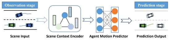
Figure 1.
An illustration of the DL-based motion prediction paradigm. The green vehicle is the target vehicle. The input here includes the historical trajectories of vehicles and the road structure, and the output is the future trajectory.
The rest of this paper is organized as follows: Section 2 first introduces the basic concepts and the basic paradigm of DL-based vehicle motion prediction methods, then discusses some current open challenges and proposes our taxonomy of recent works. Section 3, Section 4 and Section 5 review recent works based on scene input representation, context refinement, and prediction rationality improvement, respectively. Section 6 reviews the occupancy flow prediction method. Section 7 summarizes common publicly available datasets for motion prediction. Section 8 first summarizes frequently used quantitative evaluation metrics and gives a brief comparison of some state-of-the-art methods. Then, we discuss potential future research directions in this field. Finally, Section 9 presents the conclusion.
2. Basics, Challenges, and Classification
In order to help readers better understand the task of vehicle motion prediction in autonomous driving, this section first introduces the relevant concepts and terminology. After that, we describe the general implementation paradigm of DL-based vehicle motion prediction methods. Then, we discuss some open challenges currently faced in this field. Finally, we present our classification taxonomy.
2.1. Basic Concepts and Terminology
Expressions related to “motion prediction” include “behavior prediction”, “maneuver prediction”, and “trajectory prediction”. Referring to the explanation of behavior, maneuver, and trajectory in [26], we consider behavior prediction as a more general expression, which includes maneuver prediction and trajectory prediction. Trajectory prediction and maneuver prediction are more specific expressions. Trajectory prediction outputs the coordinates of the target agent’s future trajectory over a certain time. Maneuver prediction tries to infer possible future maneuvers or intentions of the target agent. Both of the two above forms focus on the individual level. In this paper, vehicle motion prediction refers to estimating motion state sets of target vehicles within a fixed length of future horizon based on the available scene information acquired by the ego vehicle. The motion prediction here includes the individual level and wide-area spatial level. At the individual level, we equal the motion prediction to the trajectory prediction, which is oriented toward individual target agents. In the wide-area spatial level, we equal the motion prediction to the occupancy flow prediction, which infers spatial occupancy around the ego vehicle.
Next, we introduce the relevant terminology of the vehicle motion prediction task. Given the scene S under the perceptible range of the ego autonomous vehicle (EV), other detected vehicles around the EV are defined as OVs. At the input level, we further divide OVs into relevant vehicles (RVs) and irrelevant vehicles (IRVs). RVs are those considered to contribute to the prediction task, and IRVs are vehicles that can be ignored at the input stage. While considering the output level, we can divide OVs into target vehicles (TVs) and non-target vehicles (NTVs), where TVs are the vehicles of interest for the motion prediction task. Occupancy flow prediction methods [29] consider the occupancy of the space around the EV and it can be therefore considered that all OVs belong to TVs. Prediction models rely on observations of OVs and the EV of a certain historical duration, and this type of input information is defined as . Different models often consider different specific observation information and have various representation forms. In addition to the dynamic motion information, many prediction models integrate with other scene information such as road structure and traffic rules, which is defined as .
2.2. Implementation Paradigm and Mathematical Expression
Deep learning-based motion prediction methods share a similar implementation paradigm, as shown in Figure 1. The model first needs to input the available scene information in the observation stage. Then, the scene context encoder encodes scene inputs and extracts the scene context feature, which is related to the future motion of TVs. After that, the motion predictor decodes the fully extracted context feature to obtain the prediction outputs. The scene context encoder and the motion predictor are often built on deep neural networks.
In order to realize the aforementioned processes, scene context encoders and motion predictors often use the following deep learning methods: Recurrent Neural Network (RNN), Convolutional Neural Network (CNN), Graph Neural Network (GNN), Attention Mechanism (AM), Generative Neural Network, and the most basic Fully Connected layer (FC). RNN is often used in the field of natural language processing and is suitable for the processing of sequential information. In vehicle motion prediction, RNN can effectively extract temporal correlation information and is often used to encode the historical motion trajectories of the inputs of each agent to extract features that represent the historical motion information. Traditional RNN is prone to gradient vanishing or gradient explosion during training, so most current work uses its improved versions: Long Short-Term Memory network (LSTM) or Gated Recurrent Unit (GRU). RNNs are also commonly used in the motion predictor to iteratively decode the motion state of a future multitemporal time step based on the extracted features of the target agents. CNN is mainly used in the image domain for its ability to capture spatial information efficiently, so some works use a CNN as the body of a scene context encoder to encode image-based inputs, as detailed in Section 3.1. There is also some work using 1D-CNN to process temporal inputs, which can be computationally faster than RNN, but is limited by the convolutional kernel size to only consider local temporal correlations. When non-Euclidean inputs are considered, GNN is often used to extract the scene context. The correlations between target objects in a real-world scene are inherently non-Euclidean; thus, GNN can efficiently extract correlations between different target nodes and facilitate the mutual transfer of information among the nodes. The GNN methods mainly include Graph Convolutional Network (GCN) and Graph Attention Network (GAT); the former is an extension of CNN, and the latter applies the Attention Mechanism (AM) to facilitate information aggregation and updating. Attention Mechanism (AM) is currently a widely used technique in motion prediction which helps the model focus on the information most relevant to the target prediction and is often used to extract the interaction information between objects (see Section 4.2). AM consists of Self-Attention Mechanism, commonly used to extract the motion information of each agent itself, and Cross-Attention Mechanism, commonly used to encode interaction features between different agents. Transformer is a typical network architecture fully utilized by AM, which extracts sufficient temporal information from a global perspective, has powerful feature encoding capabilities, and is also a popular method in the field of motion prediction at present. Generative methods, including Generative Adversarial Network (GAN) and Conditional Variational AutoEncoder (CVAE), are commonly used for multimodal trajectory generation, as detailed in Section 5.1.1. In addition, FC, as the most basic neural network, can be composed into a Multilayer Perceptron (MLP) when combined with nonlinear activation functions such as Sigmoid and ReLU. FC is often used as feature mapping or embedding encoding in scene context encoders and motion predictors. FC can also be used as the output part of the final trajectory decoding to predict the state of multiple time steps at once and in parallel.
The mathematical expression of the vehicle motion prediction task is constructed here. Under scene S, we assume that the current timestep is 0, the historical observation time span is , the futural prediction time span is , and the number of target vehicles is . The vehicle motion prediction task aims to obtain the set of motion states for the future predicted duration of TVs:
where is the predicted motion state of vehicle i at timestep t in the prediction stage. Considering the prediction uncertainty, the prediction task can be expressed in a conditional probability form: .
If the vehicle motion prediction is implemented as trajectory prediction, the predicted state of the target vehicle i at timestep t in the prediction stage is the 2D position . If the vehicle motion prediction is implemented as occupancy flow prediction, the prediction result refers to the spatial occupancy change around the EV. Specifically, the predicted state includes the occupancy grid map and the occupancy flow field . represents the occupancy of the cell area around the EV at time t, and represents the change in occupancy of the surrounding space. We will have a further explanation of the occupancy flow prediction in Section 6. As for the trajectory prediction, due to the multimodal nature of vehicle motion, many works simultaneously predict multiple state sets instead of a single deterministic output (shown in Equation (2), where K denotes the total number of modalities).
2.3. Current Open Challenges
Recent open challenges in vehicle motion prediction are discussed as follows:
- There is inter-dependency [28,30] or complex interactions [25,31,32,33] within the scene. For example, when a target vehicle wants to change lanes, it needs to consider the driving states of surrounding vehicles. Meanwhile, the lane-change actions taken by the target vehicle will also affect surrounding vehicles. Therefore, the prediction model should consider the state of TVs and the interactions in the scene.
- Another difficulty in vehicle motion prediction is that vehicle motion is multimodal [25,28,30,34,35,36]. There is hardly direct access to drivers’ intentions, and drivers tend to have different driving styles. Thus, TVs have a high degree of uncertainty of futural motion. For example, at the junction in Figure 2, the target vehicle may choose to go straight or turn right, despite consistent historical input information. Depending on the driving style, it may have different driving speeds when going straight. Many current motion prediction methods use multimodal trajectories to represent multimodality. Multimodal trajectory prediction requires the model to effectively explore modal diversity, and the set of predicted trajectories should cover trajectories close to the ground truth value.
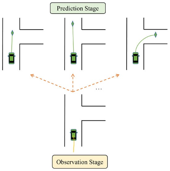 Figure 2. An illustration of the multimodal nature of a vehicle’s future motion.
 - Futural motion states of TVs are often constrained by static map elements such as lane structure and traffic rules, e.g., vehicles in right-turn lanes need to perform right turns. Thus, models should effectively integrate the map information to extract full context features related to the future motion of TVs.
- Many methods only make predictions for a single target vehicle, i.e., always equals 1. But in dense scenarios, we may need to predict the motion states of several or all vehicles around the EV. More generally, varies all the time. Therefore, models are required to predict multiple target agents jointly, and the number of TVs can be flexibly changed according to the current traffic condition. Moreover, the joint prediction of multiple agents needs to consider the mutual coordination of the future motion states of each vehicle, e.g., there should be no overlap of future trajectories between vehicles at any moment.
- DL-based methods can easily consider a variety of input information. However, as the type and number of inputs increase, the complexity of encoding input increases and may cause confusion in learning different types of information. So, the prediction model needs to efficiently and adequately represent the input scene information to better encode and extract features. Furthermore, DL-based prediction models need to extract the scene context related to the motion prediction from the pre-processed input information, and how to extract the full context feature is still an open challenge in this field.
- The practical deployment of prediction models is also a challenge. Firstly, many works assume that the model has access to the complete observation of RVs. However, the track may be missed during the actual driving process due to occlusion. Achieving accurate target vehicle prediction based on the missing input remains a problem. Secondly, many prediction methods treat the prediction function as an independent module, lacking links with other modules of autonomous driving systems. In addition, there is an issue of timeliness in practical deployment, especially for models using complex deep neural networks, which consume a large number of computational resources when running.
2.4. Classification
Mozaffari et al. [28] classify deep learning-based vehicle behavior prediction based on three criteria: input representation, output type, and prediction method. However, the classifications in [28] focus on the basic construction of the DL-based prediction model and do not consider the more refined improvements proposed by recent state-of-the-art works. For example, ref. [28] divides prediction models into Recurrent Neural Network (RNN) models, Convolutional Neural Network (CNN) models, and other DL-based models based on the neural network used in each work. Many current works use several types of neural networks at the same time, when attention should be paid to the specific problem that the use of different networks aims to solve. DL-based prediction methods have a similar implementation paradigm: the scene context encoder encodes the scene input to extract the context feature related to future motion, and then the motion predictor decodes the context feature to obtain the target predictions (see Figure 1). Facing the challenges mentioned above, many DL-based prediction methods have proposed improvements to the basic paradigm. To understand the latest exploration, this paper summarizes recent DL-based vehicle motion prediction works based on the improvements to the basic paradigm in three aspects: Scene Input Representation, Context Refinement, and Prediction Rationality Improvement. Firstly, proper scene input representation is a prerequisite for extracting the context feature. Moreover, the model cannot achieve accurate and reasonable motion prediction without a complete understanding of the scene, which requires the model to extract sufficient scene context. In addition, the predictions should be valid and have good semantic interpretability. The classification proposed in this paper is shown in Figure 3; in addition, the distribution of related works included in this paper based on this classification is shown in Table 1.
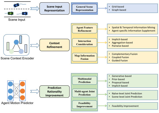
Figure 3.
The proposed classification for vehicle motion prediction methods.

Table 1.
Overall distribution of covered literature.
3. Scene Input Representation
Scene input refers to the surrounding environment information acquired within the perceptible range by the EV, including the historical motion states of traffic participants and map information. The prediction model needs to encode features based on a reasonable scene representation. Since the input becomes richer and more diverse, some works construct a general representation of all scene elements to reduce model complexity and improve the efficiency of feature extraction. We classify recent works for general scene representation into grid-based and graph-based approaches.
3.1. Grid-Based
The grid-based approach divides the region of interest into regular and uniformly sized grid cells, each of which can store information about the area, such as the encoded historical motion features of vehicles in the cell (see Figure 4). This kind of representation emphasizes the spatial proximity between scene elements and preserves scene information as richly as possible.
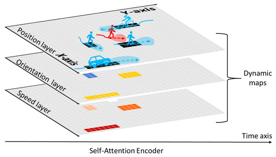
Figure 4.
An example of grid-based representation [39]. The authors design a 3-channel grid map to encode the location, orientation, and speed of traffic participants in the space around the target agent.
Refs. [35,36,37] use a bird-eye-view (BEV) raster image to represent the scene information around the target vehicle, including lane structure, traffic rules, and historical vehicle motion states. Each pixel in the raster image is a grid cell that occupies a specific area. The raster image utilizes different color properties to the pixels to represent different information, such as using different RGB colors to represent different vehicles and using different luminance values to distinguish different timesteps. Hou et al. [43] represent all scene elements in the same channel of the grid map to consider the influence of map elements or traffic rules on the movement of the target vehicle, where the value of each grid is determined by the type of object in the corresponding grid, representing the degree of danger or constraint to the target vehicle of that object. To balance the computational complexity and the integrity of information retention, the authors simultaneously construct three raster maps with different area ranges and different grid sizes centered on the target vehicle. However, considering all scene information in the same channel may cause information confusion in the model. Refs. [38,39,40,41] construct a multi-channel semantic grid map whose different channels represent different semantic information, and the grid map of each channel shares spatial proximity information. Ref. [42] represents all scene inputs in the same grid map with point-based features. Each point in [42] has its attributes such as position, velocity, heading angle, etc. Points at different timesteps are simultaneously included in the grid map by assigning different one-hot encodings. The points located in the same grid cell will be aggregated to obtain the feature map of the grid region. Then, the context feature is further extracted based on CNNs.
The grid-based representation facilitates the prediction model to capture spatial proximity relationships and more easily complements other region-based input information. In addition, the grid-based representation is often encoded based on CNNs, which have mature network frameworks that can facilitate the implementation. However, this approach often obtains actor-specific representation, which cannot be easily extended to multi-agent joint prediction. Furthermore, the convolutional kernels used in prediction models are generally not too large considering the complexity of the model, which can lead the model to ignore long-range information.
3.2. Graph-Based
The road structure is often variable and non-regular, and the interrelationships between elements within a scene are diverse, implicit, and complex. Therefore, some works use graphs to represent scenes that are good at non-Euclidean relationships (see Figure 5). The graph-based representation constructs a scene graph that can fully reflect the interrelationships of scene elements. The scene graph is composed of nodes and edges, where nodes represent specific objects and edges describe the relationships between nodes.
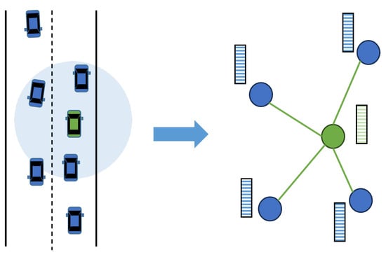
Figure 5.
An example of graph-based representation. The green vehicle is the target to be predicted, while blue vehicles belong to surrounding vehicles. A scene graph centered on the target vehicle is constructed to capture the interactions. Nodes represent agents in the scene, and an edge exists if the distance between a surrounding vehicle and the target vehicle is below a threshold.
Zhang et al. [52] constructed a graph for each timestep, where each node represents a moving vehicle. When the distance between two vehicles is less than a certain threshold, there are connected edges between the corresponding nodes. To consider map elements, refs. [46,47,48,51] use undirected fully connected graphs to represent the vehicles and lanes within the scene. They first obtain a set of vectors of motion trajectories and lane centerlines based on original input data. Each vector contains the combined information of two adjacent points of trajectories or lane centerlines. Each vector is then used as a node, and all vectors have edges between them to construct the scene graph. Deep learning networks such as GNN or the attention mechanism can then be used to encode the graph and extract the context feature. The fully connected graph is simple to construct but has a high computational cost and ignores specific semantic connections between elements. For this reason, ref. [49] defines four directed edges between lane nodes to construct a directed graph based on connectivity between lanes. Specifically, the authors construct a graph of its surrounding lanes based on each vehicle. Each graph takes lane centerline segments as nodes, and the node attributes cover not only the structure and semantic information of the lane segments but also vehicles’ motion information. Mo et al. [53] constructed a heterogeneous hierarchical graph for the scenario. The graph has two types of nodes: dynamic agents and candidate centerlines. The hierarchical graph consists of two layers. The lower layer graph models the relationships between agents and candidate centerlines, while the upper layer graph can extract the inter-agent interaction. Moreover, the authors use a sparse and convenient graph construction method. In the lower layer graph, the motion agent node is at the center, and its candidate centerline nodes are connected to it by one-way edges, representing the flow of information from the map to the agent in the bottom graph. In the upper graph, the target agent node is at the center, and the surrounding agents are connected to the target agent by one-way edges, representing the flow of information from the surrounding agents to the target agent. With this star-like and sparse graph representation, global information can be considered using the scene topology, and too-intensive computation can be avoided. The methods above do not consider the connection of nodes in the time dimension when constructing the scene graph. Thus, some methods consider the temporal connections of the nodes. Refs. [44,45,50,54] construct a spatio-temporal scene graph, which defines not only edges to connect different dynamic agents representing spatial proximity relations but also temporal edges to represent the flow of scene information with the temporal dimension.
Graph-based representation is sparser than grid-based representation, highlighting the flow of spatial–temporal information. Moreover, models can consider a more extended range of scene information by transmitting and updating node features several times. However, this approach requires predefined node connection rules, such as undirected full connection rules for agent nodes [46,47,48] and spatial connectivity connection rules for lane nodes [49,55]. It may be hard to define suitable connection rules when the scene elements are diverse with complex relationships.
See Table 2 for a summary of General Scene Representation.
Table 2.
Summary of General Scene Representation methods of recent works.
4. Context Refinement
The scene context refers to the abstract summary of scene information, i.e., the context feature related to motion prediction. Extracting the scene context cannot be separated from learning historical static and dynamic information about the scene. In terms of dynamic scene information, models often need to obtain individual agent features. In addition, the inter-dependency or interaction between vehicles should also be fully considered. In terms of static scene information, since the vehicle motion is heavily constrained by the road structure and other map elements, if the model can efficiently integrate the map information, it can improve the process of context extraction. In this subsection, we will summarize the context refinement methods from three aspects: Agent Feature Refinement, Interaction Consideration, and Map Information Fusion.
4.1. Agent Feature Refinement
DL-based prediction models need to encode individual features of dynamic agents to fully extract the scene context. The adequate extraction of agent features can facilitate the acquisition of scene context. In this subsection, we present the ways to refine the extraction of individual agent features, which can be divided into two classes: Spatial and Temporal Information Mining and Agent-specific Information Supplement.
4.1.1. Spatial and Temporal Information Mining
The moving vehicle is a spatial–temporal states carrier, and thus the prediction model requires careful consideration of agent information on both temporal and spatial dimensions [87]. Neglecting either of these two pieces of information can be detrimental to the extraction of the context feature [56].
Aiming at extracting adequate agent temporal information, Liang et al. [55] use 1D-CNNs to encode the sequence of motion states along the time dimension; then, multi-scale features are obtained and fused by using a feature pyramid network (FPN) [100]. Ye et al. [56] argue that the learning of temporal features is strongly related to the time interval considered. The authors define multiple time intervals, and aggregate agent motion states at different time intervals, followed by the multi-interval feature fusion. There are also works [44,45,57,58,59] considering temporal information by constructing spatial–temporal graphs or performing attention mechanisms in the temporal dimension.
In order to fully extract the spatial information, ref. [56] first obtains both voxel and point features based on the point cloud processing idea and then makes a fusion of the features with dual representations. When the vehicle movement is fast, or the scene is large, the model should consider the long-range dependency, which requires the model to learn a wider range of spatial information. Gilles et al. [40] use a multi-channel grid map to represent the scene. To consider long-range dependencies, the authors applied transposed CNN to extend the feature map, saving computational effort compared to directly increasing the kernel size of CNNs. In [49], based on the graph representation, the authors use a multi-order graph convolution operation to help the model learn wider spatial features.
4.1.2. Agent-Specific Information Supplement
The refinement of agent features can also consider the encoding of agent-specific information. For example, supplement the input with the category attributes of different traffic participants.
There are often multiple types of traffic participants in dense scenes, and different types of traffic participants have distinct differences in motion characteristics, so [32,44,50,57,61] consider supplementing the model with category information. Refs. [32,57,61] directly embed the category index into the input state vector of the motion agent, together with other input embeddings. Refs. [44,50] define “super nodes” representing different traffic participants’ categories in their scene graph. Specifically, different categories of traffic participants have their own super node, which is responsible for aggregating the information of all agent nodes of the corresponding category at each moment, and then updating the current super node state with the information of the previous moment. The super node transmits the updated state back to each agent node of the corresponding category, thus supplementing the information of category features under a group.
Prediction models often use neural networks with shared weights to encode features of all vehicles within a scene, but Varadarajan et al. [60] define a different feature encoder for the EV. The authors argue that the EV has distinct attributes compared to other agents and should be given special consideration. The authors construct an individual encoder to extract the motion feature of the EV and then incorporate the feature into the target vehicle feature based on the cross-attention mechanism.
The agent feature refinement methods are summarized in Table 3.
Table 3.
Summary of agent feature refinement methods of recent works.
4.2. Interaction Consideration
The interaction between agents, also referred to as inter-dependency in [28], essentially refers to the mutual influence between agents in the same space–time. Learning interaction information can help the model to refine the context feature. Current works mainly focus on obtaining features characterizing interaction information as a complement to context features. Here, methods of interaction consideration are divided into three categories: implicit-based, aggregation-based, and pairwise-based.
4.2.1. Implicit-Based
Implicit-based interaction consideration means that there is no explicit process of computing the interaction feature (see Figure 6a). However, the model indeed considers other traffic participant states around the target agent to extract the context feature. And the model defaults to the condition that the extracted context feature already contains interaction information.

Figure 6.
An illustration of interaction consideration methods: (a–c) denote implicit-based, aggregation-based, and pairwise-based methods, respectively. Numbers 1, 2, and 3 denote the agent feature encoding stage, interaction feature encoding stage, and context feature encoding stage, respectively. The implicit method has no explicit interaction feature encoding phase. In aggregation-based methods, the features of vehicles around the target vehicle are aggregated in a uniform manner such as averaging pooling to obtain the interaction feature and then concatenated with the target vehicle feature to obtain the context feature. The pairwise-based method designs agent-to-agent (A2A) modules to model the different inter-dependencies between each surrounding agent and the target agent. The A2A module is usually based on the attention mechanism.
Some grid-based representation works [35,36,37,38,64] belong to this approach. The historical motion states of all vehicles are simultaneously represented in a grid map, and the context feature is extracted based on CNNs. Since the input sequence of historical motion states can reflect the vehicle interrelationship under the scene, the interaction information can be implicitly included in the context. In order to consider the interaction between the target vehicle and the six surrounding vehicles, Zou et al. [63] concatenate the encoded target vehicle feature with the surrounding vehicle features and then directly encode them using a fully connected layer to obtain the target context feature. Refs. [62,65,66] use a similar process. The above method of representing the states of other agents in the same tensor is sensitive to the order, thus causing inadequate extraction of the interaction feature.
The implicit-based approach is easy to implement, but the drawbacks are also obvious. First, it is difficult for the model to fully consider the interactions between vehicles. Second, this approach cannot distinguish the differences in other vehicles’ influences on the target vehicle’s future motion. In addition, the interactions within a scene are complex and multidimensional, and the implicit interaction method follows a uniform idea that does not allow for a good treatment of diverse interactions.
4.2.2. Aggregation-Based
The aggregation-based approach explicitly encodes the interaction feature following a two-stage process: first encoding the motion states of each vehicle of interest and then aggregating these features (see Figure 6b) to represent the interaction influence on the target vehicle.
Alahi et al. [2] design a social pooling layer for aggregating Long Short-Term Memory Network (LSTM) encoded hidden features of nearby agents based on the spatial relationship, obtaining the interaction features in a permutation invariant way, and the authors of [68,69] use a similar approach. Gupta et al. [3] chose to encode the relative distances between surrounding agents and the target agent, followed by a maximum pooling layer. The obtained pooled feature is then collocated with the target agent motion encoding and a random noise as the context feature for trajectory decoding. Gao et al. [70] consider the influence of five other vehicles around the target vehicle. Firstly, the authors concatenate all surrounding vehicles’ longitudinal distances and velocities relative to the target vehicle into the same state vector and then obtain the representation of the surrounding vehicle aggregation feature through a fully connected layer. The aggregated interaction feature is then used to obtain the Query in the Transformer decoder attention operation to optimize the target vehicle motion feature.
Compared with the implicit-based approach, the aggregation-based approach has an explicit extracting process of the interaction feature, which mainly considers the spatial correlation. The aggregation-based method is generally based on a fixed spatial range around the target agent and does not consider long-range interactions sufficiently. In addition, this approach considers interactions among agents in a uniform way, which fails to distinguish the differences in the influence of agents.
4.2.3. Pairwise-Based
Compared to the above two approaches, the pairwise-based approach highlights different specific inter-dependencies between two agents (see Figure 6c).
For each surrounding vehicle, Guo et al. [81] calculate the relative distance between it and the target vehicle, which is then stitched with the encoded features of the surrounding vehicle and the target vehicle. The authors perform the same operation for all surrounding vehicles to be considered and then sum these encoded features up to represent the interaction with the target vehicle. Many works of this approach use the attention mechanism to help learn the interaction feature. Gilles et al. [40] first encode the motion states of the target vehicle and the surrounding vehicles to obtain features representing the respective historical information. Then, the authors use the target vehicle feature to obtain Query and use the surrounding vehicle features to obtain Keys and Values for attention operations. In a kind of one-direction information transfer way, the interactive features of surrounding vehicles are aggregated and transferred to the target vehicle. After encoding the historical information of each vehicle, refs. [31,76,79] first incorporate the map information into each vehicle by applying cross-attention and then use the attention operation among the vehicles to obtain interaction features. Yu et al. [77] first learn spatial proximity information based on the encoding of the grid map, and then the influence of different grid cells on the future motion of the target vehicle is obtained by using the attention mechanism. To fully extract the interaction information, some works [32,73] use the multi-headed attention mechanism to consider the interaction in different dimensions. Scene information which needs to be considered is often sparse and non-Euclidean, so some works also apply graphs to model interactions within the scene [44,46,47,48,52,53,54,59,61,71,72,74,75,78,82]. For example, refs. [61,82] construct a scene graph to describe the interaction between traffic participants, with different nodes representing different traffic participants, and apply GCN to achieve the transfer and aggregation of information between nodes. Refs. [52,53], on the other hand, efficiently extracted the amount of interaction features between surrounding vehicles and target vehicles by applying GAT (i.e., graph neural network incorporating the attention mechanism).
The pairwise-based approach highlights more specific interaction relationships than the previous two approaches, integrating the influence of the surrounding vehicle on the target vehicle in an efficient and integrated form. This approach often uses attention mechanisms and graph neural networks. The former is similar to the weighted sum of information about surrounding agents, while the latter focuses on aggregating, passing, and updating features of surrounding agents.
The interaction consideration methods are summarized in Table 4.
Table 4.
Summary of interaction consideration methods of recent works.
4.3. Map Information Fusion
Vehicle motion is constrained by map-relevant information such as road structures and traffic rules. More and more prediction models consider the fusion of map information to improve prediction accuracy. In this subsection, we classify different methods into complementary fusion, coupled fusion, and guided fusion in terms of fusion mode and degree. The latter two fusion methods emphasize the coupling with moving objects’ information.
4.3.1. Complementary Fusion
This type of fusion approach treats map information as an additional input supplement and encodes map information independent of other motion agents. The map feature is then directly concatenated with the target vehicle feature (see Figure 7a), which emphasizes complementing contextual information.
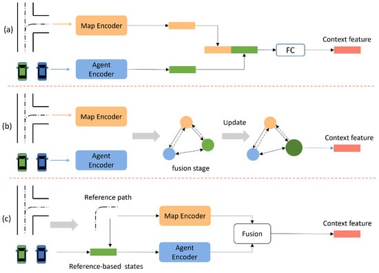
Figure 7.
An illustration of map information fusion methods. (a–c) represent complementary fusion, coupled fusion, and guided fusion, respectively.
Considering environmental elements such as roads and weather conditions, Yu et al. [77] design a constraint net to model environmental constraints. The authors embed the discrete environment elements into dense continuous vectors with the same dimension, which are then concatenated together to form the environment vector. Then, the Multi-Layer Perceptron (MLP) is used to encode the environment vector to obtain the constraint feature, which will be used to supplement contextual information for motion prediction. Huang et al. [83] mainly consider the fusion of lane information. The authors first search lane centerlines near the target vehicle and then fit them using quadratic polynomial curves. The fit coefficients are then encoded by a fully connected layer to obtain the map-relevant feature. Finally, the map-relevant feature, together with the motion feature, is input into the LSTM to extract the context feature.
Complementary fusion is easy to implement and flexible to add new map elements. However, this approach ignores the connections between map elements and vehicles. It cannot determine which specific information is directly related to the future motion of the target vehicle.
4.3.2. Coupled Fusion
The complementary fusion approach does not consider the correlation between map elements and motion agents in the scene. The coupled fusion approach aims to introduce a tighter fusion of map information with vehicle motion information (see Figure 7b).
Some works [35,36,37,38,64,85,87] represent the vehicle history motion states and map elements on a grid map and then use CNNs to encode them uniformly in order to extract the scene context. The grid map implicitly covers the correlation between vehicles and map elements. However, this fusion of map information relies on grid cell resolution, which inevitably results in information loss. Furthermore, it is hard to distinguish the influence of different lanes [84]. In order to consider the difference in the influence of different map elements, refs. [45,53,58,76,84,86] apply the attention mechanism to fuse map information with the motion of agents. Take [84] as an example: it first uses 1D-CNN and MLP to encode the centerline coordinates of the possible future lanes of the target vehicle. Then, the authors use the target vehicle’s historical trajectory to obtain Query and use lane encodings to obtain Keys and Values. The influence of different lanes on the future motion of the target vehicle is explored by calculating the attention scores based on the Query and Keys. In addition, there are works to establish interconnections between vehicles and map elements by constructing graphs. Ref. [46] constructs fully connected undirected graphs with lane centerline segments and traffic participants as nodes, then uses the attention mechanism between the nodes to pass map information rightfully to other motion agents. Ref. [55] similarly constructs the graph of the centerline segments, but defines specific directed edges based on four connectivity relationships between lane segments, from which four adjacency matrices are defined. The node state is then updated based on graph convolution operations. Ref. [55] highlights the information flow within the scene and performs information transfer between agents, from agents to lanes, between lanes, and from lanes to agents, respectively, to enhance the extraction of the global context feature. Ref. [81] also constructs a lane graph based on four connection relationships, and further, the authors couple the vehicle motion states with the map information to obtain the traffic flow information of the scene. Specifically, the authors use an attention mechanism to fuse the motion characteristics of vehicles near a lane segment node into the state of that node to represent the traffic information of that lane segment. The authors then execute the LaneGCN proposed by [55] to pass and update node states within the lane graph to obtain more global information. The road segment nodes with fused traffic flow information will be fused with the target vehicle state to obtain the full context feature.
The coupled fusion approach fuses the map information in an adequate and efficient way by emphasizing the acquisition of interrelationships between map elements and moving objects. However, this approach does not facilitate the direct extension of multiple types of map elements, and the model complexity generally increases significantly with the increase of scene elements.
4.3.3. Guided Fusion
This approach considers the fusion of lane information and is mainly used in multimodal trajectory prediction. Usually, target vehicles drive in the lanes, and thus the lanes have a guiding effect on the vehicle motion. The guided fusion approach considers the future lane of the target vehicle and uses it as a reference to constrain the vehicle state representation (see Figure 7c). The reference-based feature helps the model extract the scene context of the target vehicle while also constraining the prediction region.
Zhang et al. [88] first obtain multiple future drivable lanes based on the target vehicle location and map structure and use lane centerlines as references to guide the prediction of the future motion of the target vehicle. Then, the authors combine vehicle motion states with the features of each reference path, obtain different reference-based context features, and decode the corresponding trajectories. Tian et al. [90] use an efficient way to fuse lane information: Given the candidate centerline of the lane that the target vehicle may traverse, trajectories of all vehicles are projected on the centerline coordinate system. Based on several candidate centerlines, the authors encode multiple sets of motion states to represent different intention modes of the target vehicle. Then, the intention-based encodings, together with one-hot motion mode embeddings, are input to the LSTM decoder for multimodal trajectory decoding.
The guided fusion approach also considers the coupling of vehicle and map information but emphasizes the lane’s role in guiding the vehicle’s future motion. The guided fusion approach often requires first acquiring possible reference paths based on the target vehicle location, which also reflects the vehicle’s movement intention. So, the implementation effectiveness of this approach depends on the candidate lanes acquired in the first stage.
The map fusion methods are summarized in Table 5.
Table 5.
Summary of map information fusion methods of recent works.
5. Prediction Rationality Improvement
The prediction model should not only ensure that the prediction results of the target vehicle are physically safe and feasible but also require that the prediction results should have good semantic interpretability for real scenarios. We express such requirements as prediction rationality. Here, we summarize the improvement methods for prediction rationality based on recent works, which can be divided into three aspects: multimodal prediction, multi-agent joint prediction, and feasibility improvement.
5.1. Multimodal Prediction
Surrounding vehicles of the EV have unknowable driving intentions, and therefore the motion of target vehicles has a highly uncertain or multimodal nature. Intuitively, target vehicles with consistent historical observation states may have different future trajectories. The prediction model should be able to explain the multimodal nature, so many works output predictions that cover multiple possible sets of motion states. However, only one ground truth exists for model training, so many works for multimodal learning are based on the winner-takes-all (WTA) approach in multi-choice learning [101]. Specifically, although the output is multimodal, only one of the modes is trained for a sample, and all modes can be trained when training samples are sufficiently random and diverse. The multimodal prediction methods are divided into four classes: generative-based, prior-based, proposal-based, and implicit-based.
5.1.1. Generative-Based
The generative-based multimodal prediction follows a random sampling idea and mainly includes two methods: Generative Adversarial Network-based (GAN-based) and Conditional Variational Auto Encoder-based (CVAE-based). Specifically, GAN-based multimodal prediction methods randomly sample noise variables to represent different modes (see Figure 8a), and the noise distribution is known in advance. CVAE-based multimodal prediction methods generate latent variables related to the target vehicle’s historical and futural motion, representing motion modalities. The model needs to learn the latent variable distribution using neural networks and then samples different latent variables in the inference stage to decode the predicted multimodal trajectories (see Figure 8b).
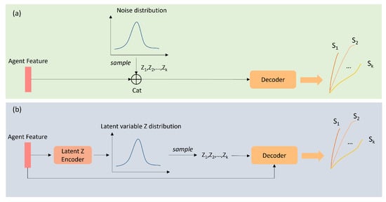
Figure 8.
A schematic diagram of generative-based multimodal prediction approach: (a,b) represents the process of generating multimodal trajectories in the inference stage by the GAN-based method and CVAE-based method, respectively. (a) the GAN-based method randomly samples the noise with known distribution (e.g., Gaussian distribution) to represent different modes. (b) the CVAE-based method needs to encode the agent feature into a low-dimensional latent variable that obeys a predefined distribution type. Different latent variables thus are sampled based on the learned distribution and are decoded along with the agent feature to predict multimodal trajectories.
Refs. [3,67,91] sample noise variables that obey the standard normal distribution and directly concatenate them with the agent motion features for multimodal trajectory decoding. Huang et al. [83] encode the agent states with the sampled noise to obtain the latent variable representing high-level semantics. The authors define appropriate training loss to ensure that different semantic latent variables correspond to distinct predicted trajectory encodings. To improve the diversity of GAN-based multimodal predictions, Ref. [83] used the Farthest Point Sampling (FPS) algorithm [102,103] to obtain semantic modalities that are as distinct as possible, resulting in trajectory sets with significant differences.
The CVAE-based methods [34,39,62,66] are another typical generative-based multimodal prediction approach. Ref. [62] constructs a low-level latent variable correlated with the historical and futural motion of the target vehicle, and defines that the distribution of the latent variable conforms to a normal distribution. The mean and standard deviation of the distribution are obtained by learning the scene context based on a neural network. Randomly sampling multiple latent variables to represent modalities in the prediction stage, the multimodal trajectories can be obtained by decoding the latent variables together with target agent motion features.
Generative-based methods are able to represent complex input information by constructing low-level latent variables to obtain multiple modes by random sampling. But it is not known how many samples can represent diverse enough modalities. Moreover, generative-based methods often lack interpretability and are prone to the “mode collapse” problem [47]. Furthermore, the multimodal trajectories obtained based on generative-based methods often do not have corresponding probability values, which harms the interpretability of predictions.
5.1.2. Prior-Based
A key problem of generative-based methods is the low interpretability and the uncertainty of the number of modes. The prior-based multimodal prediction approach specifies specific modes based on prior knowledge, such as driving maneuvers or intentions of the target vehicle (see Figure 9), and then predicts the future motion states based on each mode separately.
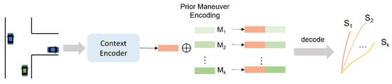
Figure 9.
A schematic diagram of prior-based multimodal prediction approach. The predefined prior maneuver encodings concatenate with the context feature of the target agent and then are decoded to generate trajectories of different maneuvers.
Refs. [68,92] achieve vehicle trajectory prediction for highway lane-change scenarios. They predefine two longitudinal maneuvers (normal driving, braking) and three lateral maneuvers (left-lane changing, right-lane changing, and lane keeping) that the target vehicle can take at the prediction stage. A total of six trajectory modes are obtained by permutation and combination of the above two types of maneuvers, which are then represented in one-hot encodings. The encoding of each modality is separately concatenated with the scene context, which is then used for future trajectory decoding. Ref. [93] uses the same idea to implement multimodal prediction but with more maneuvers. The above methods often define nets with the same inputs of context encoder to predict the probabilities of different modes.
Phan-Minh et al. [36] argue that the feasible future actions of the target vehicle in a short time are finite. So, the authors regard trajectory prediction as a classification problem in a finite trajectory set, thus avoiding the possible pattern collapse problem in direct multi-output regression. The authors sample and classify the trajectories of the training data to obtain a rich and typical set of vehicle trajectories with different modalities. However, this way of obtaining multimodal trajectories by classification is largely limited by the generation of the prior trajectory set.
The prior-based multimodal prediction methods obtain multiple outputs based on predefined maneuvers or trajectory sets and have a certain degree of interpretability. However, prior-based methods lack the capability of multi-scene generalization and are often used in highway lane-changing prediction tasks. In addition, this approach is also prone to a lack of diversity in multimodal outputs as it is hard to predefine complete priors for future motion prediction.
5.1.3. Proposal-Based
The proposal-based approach obtains “proposals” to guide the multimodal prediction process (see Figure 10). The proposals can refer to physical quantity [40,47,48,49,53,76,79,89,94,96], such as points on the lanes, or abstract quantity [60,95,97,98], such as semantic tokens. The “proposals” of motion prediction tasks can be referred to in different ways, such as “targets”, “goals”. Unlike the prior-based approach, the proposals need to be generated by the model itself based on the scene information. The models need to extract the relevant features of each proposal or modality as adequately as possible.
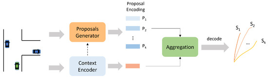
Figure 10.
A schematic diagram of proposal-based multimodal prediction approach. This approach requires the model to adaptively generate multiple proposals to represent different modalities based on the scenario information.
Zhao et al. [47] use the trajectory endpoints of the target vehicle in the prediction phase as proposals, which are not only interpretable physical points but also closely related to driving intentions. The authors first predict the trajectory endpoints based on the scene context, where different endpoints represent different modalities, then use an MLP to complement the trajectories based on different proposals. Narayanan et al. [89] extract the centerlines of lanes where the target vehicle is likely to drive in the near future. These centerlines are used as proposals and are encoded with scene information to obtain features representing different modalities. Ref. [53] predicts multiple trajectories based on the candidate centerlines of the target vehicle, which are dynamic and map-adaptive since the candidate centerlines are obtained based on the current vehicle motion states and the road topology. In addition, the authors consider adding two other trajectories: a scene reasoning trajectory and a motion-maintaining trajectory. The former aims to indicate that several lanes may influence the future trajectory of the vehicle, and the latter indicates the matching of the future trajectory with the historical motion states. The proposals generated in the works mentioned above are sparse, which may lead to neglecting modal diversity. Ref. [48] also uses the trajectory endpoints of the target agent as proposals, but uses a multi-stage densification method in obtaining the trajectory endpoints. The authors then obtain the set of trajectory endpoints containing the maximum probability of the true trajectory endpoint based on the mountain climbing algorithm. Refs. [40,76,79] generate the probabilistic heat map of the trajectory endpoints. Different endpoints are sampled from the heat map to represent different modes. To improve the efficiency of the probabilistic heat map generation, ref. [76] uses the hierarchical approach: For the regions where the target vehicles are likely to be distributed in the future, the future endpoints are first predicted based on a large grid size heatmap. The probabilistic heatmap is regenerated using smaller grid sizes for regions with higher probability on the formerly generated heatmap. Then, the operation is repeated to reach the expected resolution size.
Liu et al. [95] introduce implicit proposals to represent different modalities with no specific physical meaning. The authors wish the model to take more into account the potential features of each mode to ensure the stability of multimodal prediction. The authors use the Queries in the transformer decoder as proposals and aim to make them distinct to represent different modalities. Features of proposals in [95] are updated by hierarchical, stacked transformers, and absorb the scene information which implicitly contains modality features. The authors argue that the parallel Queries processing in the transformer allows each proposal to consider the encoder information independently, helping to construct the respective modal information.
The proposal-based multimodal prediction approach is widely used in recent works, which can easily predict probabilistic values of different modes. The proposals are often generated based on scene information such as road structure, which is dynamic in nature and therefore better suited for multiple scenarios.
5.1.4. Implicit-Based
The implicit-based multimodal approach argues that the context feature extracted by the context encoder already contains the multimodality information. Models of this type directly decode multiple possible trajectories without explicitly defining the feature extraction of each modal.
The more adopted approach in this category is to directly regress multiple predicted trajectories and their corresponding probabilities [35,55,56,58,74,80], while the training losses generally include cross-entropy classification loss of the predicted probabilities for each modality and WTA-based regression loss of the predicted trajectories. Ref. [86] defines K independent decoders based on a fully connected net to represent K modalities. Since it contains only one real label, only the parameters of a particular decoder will be updated at each training. Messaoud et al. [32] implement multimodal prediction based on the multi-headed attention mechanism. The authors design these different heads to extract features representing modal information and then decode them to generate multiple trajectories.
The implicit-based multimodal approach is formally simpler to implement but lacks interpretability. The number of modalities in this approach is fixed before the model is trained. However, it is practically hard to determine exactly how many modalities are needed for different scenarios to be appropriate.
A summary of the multimodal motion prediction methods is shown in Table 6.
Table 6.
Summary of multimodal motion prediction methods of recent works.
5.2. Multi-Agent Joint Prediction
Autonomous vehicles will face a variable number of target vehicles in real-world traffic scenarios. Although many works consider information from multiple agents in the input stage, most of them predict only one target agent at a time in the prediction stage. Joint prediction of multiple target agents is more practical. Currently, some works simultaneously predict trajectories of multiple agents, which are classified in this section as naïve joint prediction and scene-level joint prediction. The naive joint prediction approach focuses more on the output form to achieve multi-agent prediction, while the scene-level joint prediction approach focuses more on the coordination among agents in the prediction phase.
5.2.1. Naïve-Level Joint Prediction
The naïve-level joint prediction approach supposes that if the interaction information is well learned, the extracted context feature at the encoding stage already contains the futural motion information of all target agents. So, the future motion trajectories of multiple target agents are regressed directly based on the scene context. This approach needs to learn interactions between agents in the observation stage thoroughly and often designs average L2 loss for all target agents.
Refs. [71,78] argue that multi-agent trajectories can be decoded jointly based on the context feature when the interactions within the scene are fully considered. The authors extract the context feature based on the graph convolution network and then use LSTMs with shared weights to decode the future trajectories of each target agent in parallel. In addition, in the training stage, the authors calculate the loss of the predicted deviation errors of multi-agent trajectories to ensure the model is able to make joint predictions. Ngiam et al. [58] first apply the attention mechanism to extract the scene context from both spatial and temporal dimensions and then directly decode each agent’s future trajectory simultaneously based on a MLP.
Naïve-level joint prediction methods decode the trajectories of multiple target agents simultaneously. The multi-agent loss in this approach is oriented to train the model to predict multiple agents in parallel. However, this approach only considers interaction from historical information. It does not explore the coordination among the agents in the prediction stage, which may lead to invalid results (see Figure 11).
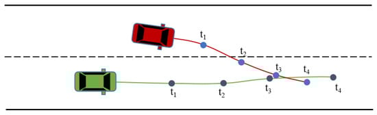
Figure 11.
An invalid result of naive multi-agent joint prediction. Due to the lack of consideration of coordination in the prediction stage, the green vehicle’s trajectory will overlap with the red vehicle’s trajectory at timestep .
5.2.2. Scene-Level Joint Prediction
The scene-level joint prediction approach emphasizes that all target agents share the same spatial–temporal scenario in the near future and highlights the coordination between the forecasting results of each target agent.
Gilles et al. [76] implement joint multimodal multi-agent prediction in two stages: First, the authors independently predict the respective multimodal trajectories of target agents and consider that the final scene-level multimodal trajectories are all already contained in this trajectory set. Then, the authors score, rank, and reorganize these independently acquired multimodal trajectories based on an attention mechanism to obtain scene-coordinated multimodal multi-agent prediction results. However, because the final predicted trajectories belong to the trajectory set, which is obtained by independent prediction of all target agents, the final predictions may ignore the more optimal multimodal combinations.
Scene-level multi-agent joint prediction takes into account the interactions of agents in the prediction stage but is more computationally intensive than naive multi-agent prediction. Both of the above two approaches require that the target vehicles are well detected and tracked in the observation stage, while in some dense traffic scenarios, the urgent target agents are often undetected due to occlusion (e.g., a sudden approaching vehicle at an intersection without detection).
The multi-agent joint prediction methods are summarized in Table 7.
Table 7.
Summary of multi-agent joint prediction methods of recent works.
5.3. Feasibility Improvement
Some works treat the prediction task as a sequence translation problem, where the inputs and outputs are usually discrete coordinate sequences of the vehicle’s center of mass. Although the predicted representations are discrete, the continuity of vehicle motion cannot be ignored. And the predicted trajectories should conform to physical constraints, such as the fact that simultaneous spatial overlap of multi-vehicle trajectories cannot occur, and the vehicles cannot travel beyond the road boundary. The solution to the above problems is called prediction feasibility improvement in this paper.
Ye et al. [96] point out that motion prediction is a streaming problem. Specifically, the authors argue that when the historical input data have a small time shift, the overlapped chunk of the input data should produce consistent prediction results. In addition, the prediction model should be robust to small spatial perturbations in the input trajectory. Therefore, the authors define a spatial–temporal consistency loss to train the model to predict trajectories with better continuity and stability. Fang et al. [22] apply the proposal-based multimodal prediction approach, and the authors first generate futural feasible reference trajectories as proposals for the target vehicle. To improve the physical feasibility of the predicted trajectories, the authors first predicted the trajectory endpoints based on neural network regression, then fitted multiple reference paths using cubic polynomial curves and eliminated the out-of-bounds paths based on the drivable area. Song et al. [31] divide the trajectory prediction process into a model-based planning stage and a deep learning-based trajectory classification stage. The trajectories generated in the first stage are consistent with the map structure as well as the current vehicle motion states and thus have better physical constraints. Furthermore, the authors can effectively reduce the computation cost since they only use DL models in the second stage to score and classify the trajectories generated in the first stage. Yao et al. [99] aim to combine deep learning-based models with physical-based models by introducing physics of traffic flow into the learning-based prediction models to improve prediction interpretability. Ref. [81] used a GAN-based prediction model. In the training phase, the authors constructed a new discriminator to constrain the feasibility of the predicted trajectories. Expressly, they set up three channels to score the predicted trajectories output by the generator: the degree of truthfulness of the predicted trajectories themselves, the matching of the predicted trajectories with the historical motion states, and the matching of the predicted trajectories with the road information. With this setting, the authors aim to facilitate the generator to predict trajectories that match its historical physical motion information and obey map constraints. Liu et al. [66], on the other hand, define an out-of-road loss to make the model generate prediction results that obey the drivable road structure.
The feasibility improvement methods are summarized in Table 8.
Table 8.
Summary of general scene representation methods of recent works.
6. Occupancy Flow Prediction
The mainstream form of vehicle motion prediction is trajectory prediction, i.e., outputting trajectory coordinates for multiple discrete timesteps. However, there are some shortcomings of trajectory-based prediction: First, the trajectory prediction depends on tracking information of the detected target vehicle. If a target vehicle is obscured and not detected by the EV, then the model cannot directly achieve trajectory prediction due to the lack of corresponding detection input. Furthermore, trajectory-based prediction is currently mainly applied for a single target vehicle and is challenging to implement scene-level multi-agent joint prediction.
Recently, there has been a new form of vehicle motion prediction: occupancy flow prediction, whose prediction output consists of the predicted occupancy grid map and the occupancy flow field (see Figure 12). The occupancy grid map is a single-channel BEV grid map of the region of interest, where each cell represents a small area, and the values in the cell between 0 and 1 represent the probability that the region is occupied by a certain part of a vehicle at a timestep. Thus, the entire occupancy grid map represents the space occupied at a given moment. Few methods only use the occupation grid map as the form of vehicle motion prediction [42,104,105] because of its inability to represent well the motion of a particular vehicle and the loss of the corresponding identity property [29]. The occupancy flow field proposed in [29] is an improvement of the occupancy grid map, which is a two-channel grid map, where each cell stores a two-dimensional displacement vector representing the motion of a certain part of a vehicle between two frames. Compared with the occupancy grid map, the occupancy flow field can describe the change of space occupancy in the scene, so it can reflect the movement of vehicles and distinguish different vehicles based on the initial position considering the occupancy change. However, the occupancy flow field cannot directly express the position of vehicles at each moment. Hence, the occupancy flow field needs to be output together with the occupancy grid map [29,106] to complement each other. Since the occupancy flow prediction is oriented to the occupancy changes in the space of the region of interest, it is even possible to predict vehicles not detected in the observation phase when the model has a good understanding of the dynamic scene [29].

Figure 12.
The output of occupancy flow prediction [29]. The left figure is the predicted occupancy grid map, indicating the specific occupancy of the space around the autonomous vehicle. The right figure is the predicted occupancy flow field, indicating the change of occupancy of the space of two adjacent keyframes.
Park et al. [104] define an occupancy grid map for the forward direction of the target vehicle to achieve trajectory prediction, which regards the trajectory prediction as a grid classification problem, while Choi et al. [105] use an occupancy grid map to reason vehicle longitudinal position. But the above works mainly serve for the trajectory prediction and are oriented towards single agent prediction. In this paper, we mainly discuss the occupancy-based prediction which is oriented towards a fixed range of area, i.e., making predictions for all moving objects around the EV.
Kim et al. [42] jointly predict the trajectory of the target agent and occupancy grid maps of the region of interest. The authors construct a BEV grid map of the region of interest around the autonomous vehicle. They use a CNN-based encoder to extract the feature map of the embedded grid and then use CNNs to predict occupancy grid maps for several keyframes. Refs. [29,106,107] jointly predict the occupancy grid map and occupancy flow field of the region of interest based on the model’s understanding of the scene. Mahjourian et al. [29] use a similar input characterization and encoding process as [42] but apply a feature pyramid network (FPN) [100] to fuse multi-scale features during decoding. Since vehicles and pedestrians have significantly different motion characteristics, ref. [29] define different decoders for vehicles and pedestrians, while the input scene information in [29] is global but ignores the motion information of individual agents. Liu et al. [106] consider the extraction of historical motion agent features and the global scene feature and then use a Swin-transformer [108] to consider the fusion of object-level features and global scene-level features. Hu et al. [107] define a hierarchical spatial–temporal network with multi-scale feature fusion to encode scene feature maps in both spatial and temporal dimensions.
Occupancy flow prediction is oriented to the occupancy changes in the space around the autonomous vehicle. However, occupancy flow prediction is a dense prediction task [42], so the model is supposed to have good learning of the scene, which requires the model not only to input as rich as possible scene information but also to possess good feature extraction capabilities, causing the model to have high complexity. Meanwhile, a higher requirement for sensors and vehicular computing devices may be required if the real-time prediction capacity is considered.
7. Public Motion Prediction Datasets
DL-based models require a large amount of data for training, so it is essential to have datasets that provide accurate, reliable, and rich traffic data. A number of institutions have built some suitable publicly available datasets. These datasets provide training samples for prediction models and serve as validation platforms to evaluate different methods. The effectiveness of different prediction algorithms can be compared and validated based on public datasets. Some datasets also hold corresponding open challenge competitions [109,110,111,112,113], which can facilitate the improvement of prediction algorithms.
Datasets used for vehicle motion prediction primarily need to provide historical tracking information. Furthermore, many datasets also provide map information. Currently, datasets vary in terms of acquisition perspective, collection sensors, frame rate, sampling scenarios, dataset size, and so on. In this paper, the datasets are divided into the aerial perspective dataset and the vehicle perspective dataset based on the perspective.
7.1. Aerial Perspective Dataset
The aerial perspective dataset has an observation viewpoint at high altitudes, with the data collection device either directly above the road (e.g., drone with cameras) or installed on the roadside (e.g., roadside cameras). The aerial perspective dataset is generated on a fixed region with no occlusion, so it can better capture the motion states of all vehicles within the scene. As the data acquisition device of the aerial perspective dataset is far away from the driving scene, it does not affect the driving vehicles within the scene and thus captures more natural driving data [114]. This kind of dataset is often based on a single vision sensor for data collection and requires good weather conditions. As a result, their sampling process is susceptible to interference from environmental factors.
NGSIM [115,116] is a widely used aerial perspective dataset published by the US Federal Highway Administration in 2006 for highway microscopic traffic flow studies. Its subsets US-101 (collected on the Hollywood Freeway section of Los Angeles) and Interstate-80 (collected on the San Francisco Freeway), are commonly used for vehicle motion prediction works for highway scenarios. NGSIM collects data by roadside cameras located 30 stories high, with a longitudinal coverage length of 500 or 640 meters and a lateral coverage including five or six lanes. However, the amount of data noise collected by NGSIM is high. HighD [114] uses a drone equipped with a high-precision camera to acquire driving data on the highway. HighD records over 110,000 vehicles, among six different scenes, with a total of 60 records. Each record has an average duration of 17 min, and each vehicle has an average appearance time of 13.6 s. HighD contains a wider speed range and higher speeds than NGSIM and has a better record for trucks. INTERACTION [117] is also collected by drones, and the scenarios collected by this dataset mainly include ramps, roundabouts, and intersections. INTERACTION spans several countries or regions with diverse driving styles. Another characteristic of INTERACTION is the high interactivity of vehicles within the scene, which poses a greater challenge to the model’s ability to extract interaction information. INTERACTION provides motion tracking information and HD maps in lanelet2 format, including road structure information and corresponding semantic information.
The commonly used aerial perspective datasets are summarized in Table 9.
Table 9.
Aerial perspective datasets.
7.2. Vehicle Perspective Dataset
The vehicle perspective dataset uses in-vehicle sensors to detect and track the surrounding traffic participants. The vehicle perspective dataset is often collected based on multiple sensors, possessing higher perception redundancy, detection accuracy, and anti-interference capability, but the corresponding implementation threshold and cost are also higher. The vehicle perspective dataset collects data with good continuity because the collection device is located in the vehicle with a natural continuous driving process, which is also more compatible with the actual driving situation. In addition, the vehicle perspective dataset is more flexible as it is not limited to a fixed area. However, vehicle perspective acquisition inevitably suffers from occlusion, which may result in the overlooking of some potential target agents. In addition, the driving behavior of a vehicle with a set of sensing devices may affect other human-driver vehicles, resulting in fewer natural motion data being recorded.
NuScenes [121] is the first dataset using a complete suite of sensors, including six cameras, five radars, and one lidar, covering a 360-degree perception region around the vehicle. The NuScenes prediction dataset was collected in Singapore and Boston in dense urban scenarios. It records over 1000 scenes of 20 s duration and provides 3D coordinates, size, orientation, and map information of traffic participants. Argoverse [122,123] is built for research on tracking and trajectory prediction in autonomous driving, which provides two versions of motion prediction dataset: Argoverse 1 Motion Forecasting dataset [122] and Argoverse 2 Motion Forecasting dataset [123]; the latter is an upgrade of the former, containing richer data and more scenarios. Argoverse contains a variety of scenarios that are of great interest for autonomous driving: driving at intersections, unprotected turning, changing lanes, etc. Argoverse not only provides history tracking information but also provides HD maps. The Waymo Open Motion Dataset (WOMD) [124] is a dataset mainly for dense urban driving with rich and challenging data records. WOMD possesses complex interaction and includes many critical situations such as merging, overtaking, unprotected turning, and so on. Furthermore, there are often multiple types of traffic participants at the same time in WOMD. WOMD is collected by five LiDAR and five high-resolution pinhole cameras, providing a total data duration of over 570 h.
The commonly used vehicle perspective datasets are summarized in Table 10.
Table 10.
Vehicle perspective datasets.
8. Evaluation Metrics and Future Potential Directions
Vehicle motion prediction algorithms should be evaluated reasonably. This section first introduces some commonly used quantitative evaluation metrics. The metrics are divided into two categories: trajectory-based and occupancy-based. The former is oriented to trajectory prediction, and the latter is for occupancy flow prediction. Then, we will compare the effectiveness of some state-of-the-art prediction methods based on several quantitative metrics. Finally, potential future research directions will be discussed.
8.1. Trajectory-Based Metrics
8.1.1. Displacement Metrics for Single-Modal Prediction
Commonly used displacement error metrics for single-modal trajectory prediction include Final Displacement Error, Average Displacement Error, Root Mean Square Error, and Mean Absolute Error.
- Final Displacement Error (FDE): This metric calculates the L2 distance between the predicted trajectory end point and the ground truth end point:where represent the predicted 2D endpoint of a TV, subscript is the total number of timesteps in the prediction horizon, and superscript represents the ground truth value. The trajectory endpoint is related to the TV’s driving intention, so it is important to evaluate the accuracy of the endpoint prediction.
- Average Displacement Error (ADE): It is used to measure the overall distance deviation of the predicted trajectory to the ground truth trajectory:where represent the predicted point at timestep t. The same variables are used in later formulas.
- Root Mean Square Error (RMSE): This metric is the average recalculation of the sum of squared distances of total timesteps from a single predicted trajectory to the ground truth trajectory:
- Mean Absolute Error (MAE): It is the average absolute error between the predicted trajectory and the ground truth trajectory, and is generally used in the horizontal and vertical directions:
8.1.2. Displacement Metrics for Multimodal Prediction
The evaluation metrics commonly used for multimodal trajectory prediction include , , , and , where K denotes the total number of modes in the final output.
means the minimum FDE among K predicted trajectories. Similarly, means the minimum ADE among K predicted trajectories. In Argoverse[122], corresponds to the ADE of the predicted trajectory with the minimum FDE value, which aims to ensure the consistency of the optimal predicted trajectory. and are proposed by [123], which add to and , respectively. p is the predicted probability of the optimal predicted trajectory. The optimal trajectory with the highest probability should be as close as possible to the ground truth trajectory.
8.1.3. Displacement Metrics for Multi-Agent Joint Prediction
When there are multiple target agents that need to be predicted, the corresponding evaluation metrics include , , , and . These metrics are expansions of the corresponding metrics in single target agent tasks, which specifically represent the average value under multiple target objects.
8.1.4. Other Metrics for Trajectory Prediction
Besides displacement error metrics for evaluating from a spatial closeness perspective, other metrics are required to further test the other prediction abilities, such as the prediction stability, the generalization ability, and the physical feasibility.
- Miss Rate (MR): If the predicted trajectory’s endpoint deviation from the true endpoint exceeds a threshold d for a sample, that sample is called a miss. The ratio of the total number of misses m to all samples M is called the miss rate. MR reflects the overall closeness of the model’s prediction of the trajectory endpoint. There are different ways of defining the distance threshold d, e.g., refs. [110,112] use a predefined fixed distance value. However, the endpoint bias tends to increase with the prediction horizon because the longer the time, the higher the motion uncertainty. In addition, the initial velocity also has an influence on the endpoint deviation. Therefore, ref. [124] defined the distance threshold based on the prediction horizon and initial velocity of the target agent. The longer the prediction horizon and the larger the initial velocity, the deviation threshold will be set larger.
- Overlap Rate (OR): OR places higher demands on the physical feasibility of the prediction model. If the predicted trajectory of a specific agent overlaps geometrically with another agent at any timestep in the prediction stage, this predicted trajectory is said to have an overlapping [124], and the OR refers to the ratio of the total number of overlapped trajectories to the trajectories of all predicted agents. The dataset has to provide the size and orientation of the detected objects to determine whether the overlapping events occur or not.
- Mean Average Precision (mAP): WOMD [124] introduces this metric which is often used in the object detection task to help test the multimodal trajectory prediction effect. Ref. [124] first groups the target agents according to the shape of their future trajectories (e.g., straight trajectories, left-turn trajectories, etc.), and then first calculates mAP within each group. Each agent has only one True Positive (TP) predicted trajectory, which is obtained based on MR, and if more than one trajectory meets the MR threshold, the one with the highest confidence is taken as the TP. The multimodal prediction trajectories of target agents are sorted by probability value, and the accuracy and recall of each prediction trajectory can be obtained from the highest to the lowest confidence level. Then, the mAP can be calculated similarly in the object detection task. The mAP value for each group is obtained and then averaged over all groups as the final result.
8.2. Occupancy-Based Metrics
- Area Under the Curve (AUC): In [29,42,106], AUC is used to evaluate the predicted occupancy grid map, obtaining the predicted occupancy grid map and the ground truth occupancy grid map at t. Each cell in has the probability of being occupied, while each cell in is 0 or 1, indicating whether the object is partially occupied. A set of linearly spaced thresholds in [0,1] is selected, the PR curve is plotted based on these thresholds, and then the AUC is obtained by calculating the area under the curve.
- Soft-Intersection-over-Union (Soft-IoU): This metric calculates the intersection ratio of predicted occupancy grid map and the ground truth occupancy grid map at keyframe t.
- End Point Error (EPE): This metric can evaluate the effectiveness of the predicted occupancy flow field . The cells in store the 2D motion vectors for the corresponding cell grid at t. The EPE then calculates the mean square error of the motion vector in the for the corresponding region based on the cells with non-zero occupancy. As shown in Equation (9), where denotes the occupancy flow field at keyframe t (the predicted one is , and the ground truth is ) and M denotes the total number of cells with Non-Zero GT occupancy.
- In addition, the occupancy flow depicts the change of the occupancy between two keyframes so that the occupancy flow can be evaluated in combination with the occupied grid. Ref. [29] uses and of the previous frame to recover the occupancy grid map of the current frame. Then, the metrics and Soft-IoU are calculated with the true occupancy grid at current keyframe t.
8.3. Comparison of State-of-the-Art Methods
The training and validation of deep learning prediction algorithms are dataset-dependent. Different datasets may have distinct evaluation metrics, making it difficult to directly compare all methods. This subsection will compare some state-of-the-art methods based on three frequently used datasets: Argoverse, WOMD, and INTERACTION, as shown in Table 11, Table 12 and Table 13. Note that we only compare the multimodal trajectory prediction for a single target vehicle, and the number of modalities is six. The bolded values in these tables represent the optimal values under the corresponding metrics.
Table 11.
Comparison of some state-of-the-art methods based on the Argoverse 1 MF dataset (Data in bold represent that metric’s optimal value in the table).
Table 11 compares some state-of-the-art methods based on the Argoverse 1 Motion Forecast Dataset. Their observation horizon and prediction horizon are 2 s and 3 s, respectively. The selected metrics are minADE, minFDE, and MR (the distance threshold of MR is 2 m). Different methods are sorted in descending order by minADE, and the smaller value can indicate a better result. In Table 11, DCMS [96] (published in 2022) exhibits the best prediction results with minADE of 0.77 m, minFDE of 1.14 m, and MR of 0.11. DCMS is designed with a spatio-temporal constrained loss to facilitate the model’s prediction feasibility. In addition, the DCMS follows a two-stage trajectory prediction approach, which firstly generates multi-goals to obtain preliminary predicted candidate trajectories in a proposal-based way (see Section 5.1.3). Then, in the second stage, it outputs the deviation value and probability of each candidate trajectory based on FC using the candidate trajectories and the historical trajectories as inputs. Finally, it takes the sum of the candidate trajectories and the deviation value as the final trajectory output. Table 12 holds the comparison based on the Waymo Open Motion Dataset. The observation horizon and the prediction horizon are 1.1 s and 8 s, respectively. The selected metrics include mAP, minADE, minFDE, and MR (the distance threshold of MR is 2 m). The table is sorted in ascending order by the value of mAP, and the larger value can indicate a better result. In Table 12, MTRA [51] (published in 2022) shows the best prediction with mAP of 0.45, minADE of 0.56 m, minFDE of 1.13 m, and MR of 0.12. The method is based on the Transformer architecture to realize multimodal trajectory prediction, which shows the capability of Transformer to fully extract the scene context information. The above two datasets are both collected from a vehicle perspective. Table 13 presents the comparison by using the aerial perspective dataset: INTERACTION, with the same metrics and ranking approach used in Table 11, but the observation horizon and the prediction horizon here are 1 s and 3 s correspondingly. In Table 13, StopNet [42] (published in 2022) has the best results with minADE of 0.20 m, minFDE of 0.58 m, and MR of 0.02. This method is the first joint occupancy grid and trajectory prediction method, which takes grid-based point-wise scene elements as inputs, references PointPillars [126] to whole scene feature encoding, and applies Multipath [94] decoding part to accomplish per-agent trajectory prediction. In addition, Table 14 further compares the models in Table 11 and Table 12, including the mainly used DL methods, the observation and prediction horizon, and the training equipment mentioned in the paper.
Table 12.
Comparison of some state-of-the-art methods based on the WOMD dataset (Data in bold represent that metric’s optimal value in the table).
Table 12.
Comparison of some state-of-the-art methods based on the WOMD dataset (Data in bold represent that metric’s optimal value in the table).
| Models | Classification of Improvement Design | Metrics (K = 6) | |||||
|---|---|---|---|---|---|---|---|
| Scene Input Representation | Context Refinement | Prediction Rationality Improvement | mAP | minADE | minFDE | MR | |
| StopNet [42] | General Scene Representation | Interaction Consideration, Map Information Fusion | Multimodal Prediction | - | 0.51 | 1.49 | 0.38 |
| SceneTransformer [58] | - | Interaction Consideration | Multimodal Prediction, Multi-agent Joint Prediction | 0.28 | 0.61 | 1.21 | 0.16 |
| DenseTNT [48] | General Scene Representation | Interaction Consideration, Map Information Fusion | Multimodal Prediction | 0.33 | 1.04 | 1.55 | 0.18 |
| MPA [97] | - | Interaction Consideration, Map Information Fusion | Multimodal Prediction | 0.39 | 0.59 | 1.25 | 0.16 |
| Multipath [94] | General Scene Representation | Interaction Consideration | Multimodal Prediction | 0.41 | 0.88 | 2.04 | 0.34 |
| Golfer [80] | - | Interaction Consideration, Map Information Fusion | Multimodal Prediction | 0.41 | 0.55 | 1.16 | 0.14 |
| Multipath++ [60] | - | Interaction Consideration, Map Information Fusion, Agent Feature Refinement | Multimodal Prediction | 0.41 | 0.56 | 1.16 | 0.13 |
| MTRA [51] | - | Interaction Consideration, Map Information Fusion | Multimodal Prediction | 0.45 | 0.56 | 1.13 | 0.12 |
Table 13.
Comparison of some state-of-the-art methods based on the INTERACTION dataset (Data in bold represent that metric’s optimal value in the table).
Table 13.
Comparison of some state-of-the-art methods based on the INTERACTION dataset (Data in bold represent that metric’s optimal value in the table).
| Models | Classification of Improvement Design | Metrics (K = 6) | ||||
|---|---|---|---|---|---|---|
| Scene Input Representation | Context Refinement | Prediction Rationality Improvement | minADE | minFDE | MR | |
| DenseTNT [48] | General Scene Representation | Interaction Consideration, Map Information Fusion | Multimodal Prediction | 0.43 | 0.80 | 0.06 |
| Multipath [94] | General Scene Representation | Interaction Consideration | Multimodal Prediction | 0.32 | 0.88 | - |
| TNT [47] | General Scene Representation | Interaction Consideration, Map Information Fusion | Multimodal Prediction | 0.21 | 0.67 | - |
| GOHOME [79] | - | Interaction Consideration | Multimodal Prediction | 0.20 | 0.60 | 0.05 |
| StopNet [42] | General Scene Representation | Interaction Consideration, Map Information Fusion | Multimodal Prediction | 0.20 | 0.58 | 0.02 |
| Model | Works | Year | DL-Approaches | Observation Horizon | Prediction Horizon | Training Device |
|---|---|---|---|---|---|---|
| MTP | [35] | 2019 | CNN, FC | 2 s | 3 s | Nvidia Titan X GPU × 16 |
| Multipath | [94] | 2019 | CNN | 1.1 s | 8s | - |
| TPNet | [22] | 2020 | CNN, MLP | 2–3.2 s | 3–4.8 s | - |
| DiversityGAN | [83] | 2020 | LSTM, GAN | 2 s | 3 s | Nvidia Tesla V100 GPU × 1 |
| chenxu | [84] | 2020 | LSTM, 1D-CNN, MLP | 2 s | 3 s | - |
| SAMMP | [73] | 2020 | LSTM, AM | 2–3 s | 3–5 s | - |
| TNT | [47] | 2020 | GNN, AM, MLP | 2 s | 3 s | - |
| WIMP | [74] | 2020 | LSTM, GNN, AM | 2 s | 3 s | - |
| LaneGCN | [55] | 2020 | GCN, 1D-CNN, FPN | 2 s | 3 s | Nvidia Titan X GPU × 4 |
| PRIME | [31] | 2021 | LSTM, AM | 2 s | 3 s | - |
| HOME | [40] | 2021 | CNN, GRU, AM | 2 s | 3 s | - |
| THOMAS | [76] | 2021 | 1D-CNN, GRU, AM | 1 s | 3 s | - |
| LaneRCNN | [49] | 2021 | 1D-CNN, GNN, MLP | 2 s | 3 s | - |
| mmTransformer | [95] | 2021 | Transformer | 2 s | 3 s | - |
| DenseTNT | [48] | 2021 | GNN, AM, MLP | 1.1–2 s | 3–8 s | - |
| TPCN | [56] | 2021 | CNN, MLP | 2 s | 3 s | - |
| SceneTransformer | [58] | 2021 | Transformer | 2 s | 3 s | Nvidia Tesla V100 GPU × 1 |
| GOHOME | [79] | 2022 | 1D-CNN, GRU, GCN, AM | 2 s | 3–6 s | - |
| StopNet | [42] | 2022 | CNN | 1.1–2 s | 3–8 s | - |
| Multipath++ | [60] | 2022 | LSTM, MLP | 1.1–2 s | 3–8 s | - |
| DCMS | [96] | 2022 | CNN, MLP | 2 s | 3 s | - |
| MPA | [97] | 2022 | LSTM, MLP | 1.1 s | 8 s | |
| Golfer | [80] | 2022 | Transformer | 1.1 s | 8 s | - |
| MTRA | [51] | 2022 | Transformer | 1.1 s | 8 s | - |
| xiaoxu | [53] | 2023 | GAT, GRU | 2 s | 3 s | Nvidia RTX 2080 Ti GPU × 1 |
| ME-GAN | [81] | 2023 | GAN, FPN | 2 s | 3 s | Nvidia RTX 3090 GPU × 1 |
| MTR++ | [127] | 2023 | Transformer | 1.1 s | 8 s | GPU × 8 (No specific type) |
From the above results, we can see that, though evaluated on the same metrics, the results of the same model differ on different datasets. The reasons are twofold: On the one hand, different datasets have distinct data characteristics and prediction difficulties. On the other hand, the models have limited generalizability. Furthermore, StopNet [42] which is based on the joint prediction of the occupancy grid map and trajectory, shows great results on all three datasets, highlighting the potential of occupancy-related prediction.
8.4. Discussion of Future Directions
Deep learning-based vehicle motion prediction algorithms have developed a lot, and some state-of-the-art methods achieve high accuracy in the benchmarks. This subsection will discuss further possible research directions in this field.
- Many methods only consider single-target agent prediction, while multi-agent joint prediction has more significance in practice. Though there are some multi-agent joint prediction works [58,72,78], few of them consider the coordination of the agents’ motion in the prediction phase well, which may cause invalid outputs, e.g., trajectories of multiple target vehicles overlap in the same future timestep. Therefore, the prediction model should realize multi-agent joint prediction with full consideration of the interaction in both historical and future stages and should ensure the coordination between the predicted motion states in the future.
- Most prediction methods default the target vehicles with complete historical tracking. Nevertheless, in actual cases, the sensors will inevitably encounter the problem of occlusion so that the motion inputs may be mutilated. Therefore, future prediction works should consider this problem of residual input due to perceptual failures.
- Many deep learning-based prediction models are trained and validated on a single specific dataset and may become less effective when validated on other datasets. Autonomous vehicles may often meet unfamiliar scenarios. Thus, the generalization capability of the models also needs to be improved in the future.
- Most current approaches treat the motion prediction function as a stand-alone module, ignoring the link between prediction and other functions of autonomous driving. In the future, the close coupling between the prediction module and other modules should be further considered, such as coupling the motion prediction of surrounding vehicles with the EV’s decision-making and planning. What is more, a joint evaluation platform for prediction and decision-making can also be built.
- Occupancy flow prediction is a new form of motion prediction that aims to reason about the spatial occupancy around the EV. Occupancy flow prediction has the ability to estimate traffic dynamics, and it can even predict occluded vehicles or suddenly appearing vehicles, which is hardly possible in the form of trajectory prediction. Such models currently rely on rich inputs and complex neural networks and thus may fall short in real-time performance. Therefore, future occupancy flow prediction models should consider how to efficiently extract contextual features that can adequately characterize changes in the surrounding traffic dynamics while ensuring real-time model operation.
- Existing deep learning-based prediction methods focus on improving model prediction accuracy, but few works have adequately evaluated the timeliness of inference of prediction models. Future benchmark datasets related to vehicle motion prediction should contain quantitative metrics that could adequately evaluate the computational efficiency of models.
- Current deep learning-based prediction models characterize prediction uncertainty in two main ways: one is to output the Gaussian distribution parameters of the target vehicle states at each time step, i.e., the position mean and its covariance, such as MHA-LSTM [32]. The other is to consider multimodal outputs to simultaneously predict multiple trajectories and their probabilities, such as DenseTNT [48]. Current work based on deep learning mainly measures model uncertainty from the perspective of resultant outputs. It is often based on a priori knowledge, such as predefining a finite number of modalities. In the future, prediction uncertainty should be better considered from a modeling perspective, e.g., deep learning methods can be combined with probabilistic modeling methods.
9. Conclusions
Vehicle motion prediction helps autonomous vehicles make more efficient decisions and plans and perform more accurate and comfortable active braking by providing the future motion states of surrounding vehicles. This module can improve the safety of autonomous vehicles while reducing their energy consumption, thus contributing to the sustainability of autonomous driving. Recently, deep learning-based methods have become increasingly popular due to their adeptness with complex information and long-term forecasting. Many works have recently made improvements to the basic DL-based implementation paradigm. In order to examine the latest exploration of DL-based methods, we review recent DL-based vehicle motion prediction methods and propose a taxonomy based on their improvements to the basic paradigm. The taxonomy includes three criteria: scene input representation, context refinement, and prediction rationality improvement. While trajectory prediction is the major form of motion prediction, we also discuss the occupancy flow prediction method. Furthermore, commonly used public datasets and evaluation metrics are presented, and the performance of some state-of-the-art models has been compared based on three datasets. Despite the recent encouraging advances in vehicle motion prediction, some potential directions have been discussed in this paper.
This paper mainly discusses the prediction methods based on deep learning. In recent years, the rapid development of reinforcement learning (RL) has provided a new implementation of vehicle motion prediction, and we will continue to focus on the work of motion prediction based on reinforcement learning in the future.
Author Contributions
Conceptualization, R.H. and G.Z.; writing—original draft preparation, R.H.; writing—review and editing, R.H., G.Z., S.L. and W.T.; visualization, R.H.; supervision, G.Z. and L.X.; funding acquisition, L.X. All authors have read and agreed to the published version of the manuscript.
Funding
This research was supported in part by the Fundamental Research Funds for the Central Universities, in part by the National Natural Science Foundation of China under Grant U19A2069.
Institutional Review Board Statement
Not applicable.
Informed Consent Statement
Not applicable.
Data Availability Statement
Not applicable.
Conflicts of Interest
The authors declare no conflict of interest.
References
- Hussain, R.; Zeadally, S. Autonomous cars: Research results, issues, and future challenges. IEEE Commun. Surv. Tutor. 2018, 21, 1275–1313. [Google Scholar] [CrossRef]
- Alahi, A.; Goel, K.; Ramanathan, V.; Robicquet, A.; Fei-Fei, L.; Savarese, S. Social lstm: Human trajectory prediction in crowded spaces. In Proceedings of the IEEE Conference on Computer Vision and Pattern Recognition, Las Vegas, NV, USA, 26 June–1 July 2016; pp. 961–971. [Google Scholar]
- Gupta, A.; Johnson, J.; Fei-Fei, L.; Savarese, S.; Alahi, A. Social gan: Socially acceptable trajectories with generative adversarial networks. In Proceedings of the IEEE Conference on Computer Vision and Pattern Recognition, Salt Lake City, UT, USA, 18–22 June 2018; pp. 2255–2264. [Google Scholar]
- Xue, H.; Huynh, D.Q.; Reynolds, M. Bi-prediction: Pedestrian trajectory prediction based on bidirectional LSTM classification. In Proceedings of the 2017 International Conference on Digital Image Computing: Techniques and Applications (DICTA), Sydney, Australia, 29 November–1 December 2017; pp. 1–8. [Google Scholar]
- Zhang, P.; Ouyang, W.; Zhang, P.; Xue, J.; Zheng, N. Sr-lstm: State refinement for lstm towards pedestrian trajectory prediction. In Proceedings of the IEEE/CVF Conference on Computer Vision and Pattern Recognition, Long Beach, CA, USA, 16–20 June 2019; pp. 12085–12094. [Google Scholar]
- Zhou, Y.; Wu, H.; Cheng, H.; Qi, K.; Hu, K.; Kang, C.; Zheng, J. Social graph convolutional LSTM for pedestrian trajectory prediction. IET Intell. Transp. Syst. 2021, 15, 396–405. [Google Scholar] [CrossRef]
- Saleh, K.; Hossny, M.; Nahavandi, S. Cyclist trajectory prediction using bidirectional recurrent neural networks. In Proceedings of the AI 2018: Advances in Artificial Intelligence: 31st Australasian Joint Conference, Wellington, New Zealand, 11–14 December 2018; pp. 284–295. [Google Scholar]
- Gao, H.; Su, H.; Cai, Y.; Wu, R.; Hao, Z.; Xu, Y.; Wu, W.; Wang, J.; Li, Z.; Kan, Z. Trajectory prediction of cyclist based on dynamic Bayesian network and long short-term memory model at unsignalized intersections. Sci. China Inf. Sci. 2021, 64, 172207. [Google Scholar] [CrossRef]
- Rudenko, A.; Palmieri, L.; Herman, M.; Kitani, K.M.; Gavrila, D.M.; Arras, K.O. Human motion trajectory prediction: A survey. Int. J. Robot. Res. 2020, 39, 895–935. [Google Scholar] [CrossRef]
- Sighencea, B.I.; Stanciu, R.I.; Căleanu, C.D. A review of deep learning-based methods for pedestrian trajectory prediction. Sensors 2021, 21, 7543. [Google Scholar] [CrossRef]
- Ridel, D.; Rehder, E.; Lauer, M.; Stiller, C.; Wolf, D. A literature review on the prediction of pedestrian behavior in urban scenarios. In Proceedings of the 2018 21st International Conference on Intelligent Transportation Systems (ITSC), Maui, HI, USA, 4–7 November 2018; pp. 3105–3112. [Google Scholar]
- Ammoun, S.; Nashashibi, F. Real time trajectory prediction for collision risk estimation between vehicles. In Proceedings of the 2009 IEEE 5th International Conference on Intelligent Computer Communication and Processing, Cluj-Napoca, Romania, 27–29 August 2009; pp. 417–422. [Google Scholar]
- Kaempchen, N.; Weiss, K.; Schaefer, M.; Dietmayer, K.C. IMM object tracking for high dynamic driving maneuvers. In Proceedings of the IEEE Intelligent Vehicles Symposium, Parma, Italy, 14–17 June 2004; pp. 825–830. [Google Scholar]
- Jin, B.; Jiu, B.; Su, T.; Liu, H.; Liu, G. Switched Kalman filter-interacting multiple model algorithm based on optimal autoregressive model for manoeuvring target tracking. IET Radar Sonar Navig. 2015, 9, 199–209. [Google Scholar] [CrossRef]
- Dyckmanns, H.; Matthaei, R.; Maurer, M.; Lichte, B.; Effertz, J.; Stüker, D. Object tracking in urban intersections based on active use of a priori knowledge: Active interacting multi model filter. In Proceedings of the 2011 IEEE Intelligent Vehicles Symposium (IV), Baden-Baden, Germany, 5–9 June 2011; pp. 625–630. [Google Scholar]
- Laugier, C.; Paromtchik, I.E.; Perrollaz, M.; Yong, M.; Yoder, J.D.; Tay, C.; Mekhnacha, K.; Nègre, A. Probabilistic analysis of dynamic scenes and collision risks assessment to improve driving safety. IEEE Intell. Transp. Syst. Mag. 2011, 3, 4–19. [Google Scholar] [CrossRef]
- Qiao, S.; Shen, D.; Wang, X.; Han, N.; Zhu, W. A self-adaptive parameter selection trajectory prediction approach via hidden Markov models. IEEE Trans. Intell. Transp. Syst. 2014, 16, 284–296. [Google Scholar] [CrossRef]
- Kumar, P.; Perrollaz, M.; Lefevre, S.; Laugier, C. Learning-based approach for online lane change intention prediction. In Proceedings of the 2013 IEEE Intelligent Vehicles Symposium (IV), Gold Coast, Australia, 23–26 June 2013; pp. 797–802. [Google Scholar]
- Aoude, G.S.; Luders, B.D.; Lee, K.K.; Levine, D.S.; How, J.P. Threat assessment design for driver assistance system at intersections. In Proceedings of the 13th International IEEE Conference on Intelligent Transportation Systems, Funchal, Portugal, 19–22 September 2010; pp. 1855–1862. [Google Scholar]
- Schreier, M.; Willert, V.; Adamy, J. Bayesian, maneuver-based, long-term trajectory prediction and criticality assessment for driver assistance systems. In Proceedings of the 17th International IEEE Conference on Intelligent Transportation Systems (ITSC), Qingdao, China, 8–11 October 2014; pp. 334–341. [Google Scholar]
- Schreier, M.; Willert, V.; Adamy, J. An integrated approach to maneuver-based trajectory prediction and criticality assessment in arbitrary road environments. IEEE Trans. Intell. Transp. Syst. 2016, 17, 2751–2766. [Google Scholar] [CrossRef]
- Fang, L.; Jiang, Q.; Shi, J.; Zhou, B. Tpnet: Trajectory proposal network for motion prediction. In Proceedings of the IEEE/CVF Conference on Computer Vision and Pattern Recognition, Virtual, 14–19 June 2020; pp. 6797–6806. [Google Scholar]
- Lefèvre, S.; Vasquez, D.; Laugier, C. A survey on motion prediction and risk assessment for intelligent vehicles. ROBOMECH J. 2014, 1, 1–14. [Google Scholar] [CrossRef]
- Gomes, I.; Wolf, D. A review on intention-aware and interaction-aware trajectory prediction for autonomous vehicles. TechRxiv 2022. [Google Scholar] [CrossRef]
- Leon, F.; Gavrilescu, M. A review of tracking and trajectory prediction methods for autonomous driving. Mathematics 2021, 9, 660. [Google Scholar] [CrossRef]
- Karle, P.; Geisslinger, M.; Betz, J.; Lienkamp, M. Scenario understanding and motion prediction for autonomous vehicles-review and comparison. IEEE Trans. Intell. Transp. Syst. 2022, 23, 16962–16982. [Google Scholar] [CrossRef]
- Huang, Y.; Du, J.; Yang, Z.; Zhou, Z.; Zhang, L.; Chen, H. A Survey on Trajectory-Prediction Methods for Autonomous Driving. IEEE Trans. Intell. Veh. 2022, 7, 652–674. [Google Scholar] [CrossRef]
- Mozaffari, S.; Al-Jarrah, O.Y.; Dianati, M.; Jennings, P.; Mouzakitis, A. Deep learning-based vehicle behavior prediction for autonomous driving applications: A review. IEEE Trans. Intell. Transp. Syst. 2020, 23, 33–47. [Google Scholar] [CrossRef]
- Mahjourian, R.; Kim, J.; Chai, Y.; Tan, M.; Sapp, B.; Anguelov, D. Occupancy flow fields for motion forecasting in autonomous driving. IEEE Robot. Autom. Lett. 2022, 7, 5639–5646. [Google Scholar] [CrossRef]
- Kolekar, S.; Gite, S.; Pradhan, B.; Kotecha, K. Behavior prediction of traffic actors for intelligent vehicle using artificial intelligence techniques: A review. IEEE Access 2021, 9, 135034–135058. [Google Scholar] [CrossRef]
- Song, H.; Luan, D.; Ding, W.; Wang, M.Y.; Chen, Q. Learning to predict vehicle trajectories with model-based planning. In Proceedings of the Conference on Robot Learning, London, UK, 8–11 November 2021; pp. 1035–1045. [Google Scholar]
- Messaoud, K.; Yahiaoui, I.; Verroust-Blondet, A.; Nashashibi, F. Attention based vehicle trajectory prediction. IEEE Trans. Intell. Veh. 2020, 6, 175–185. [Google Scholar] [CrossRef]
- Casas, S.; Gulino, C.; Liao, R.; Urtasun, R. Spagnn: Spatially-aware graph neural networks for relational behavior forecasting from sensor data. In Proceedings of the 2020 IEEE International Conference on Robotics and Automation (ICRA), Paris, France, 31 May–31 August 2020; pp. 9491–9497. [Google Scholar]
- Tang, C.; Salakhutdinov, R.R. Multiple futures prediction. In Advances in Neural Information Processing Systems; Springer: Berlin/Heidelberg, Germany, 2019; Volume 32. [Google Scholar]
- Cui, H.; Radosavljevic, V.; Chou, F.C.; Lin, T.H.; Nguyen, T.; Huang, T.K.; Schneider, J.; Djuric, N. Multimodal trajectory predictions for autonomous driving using deep convolutional networks. In Proceedings of the 2019 International Conference on Robotics and Automation (ICRA), Montreal, QC, Canada, 20–24 May 2019; pp. 2090–2096. [Google Scholar]
- Phan-Minh, T.; Grigore, E.C.; Boulton, F.A.; Beijbom, O.; Wolff, E.M. Covernet: Multimodal behavior prediction using trajectory sets. In Proceedings of the IEEE/CVF Conference on Computer Vision and Pattern Recognition, Virtual, 14–19 June 2020; pp. 14074–14083. [Google Scholar]
- Djuric, N.; Radosavljevic, V.; Cui, H.; Nguyen, T.; Chou, F.C.; Lin, T.H.; Schneider, J. Short-Term Motion Prediction of Traffic Actors for Autonomous Driving Using Deep Convolutional Networks; Uber Advanced Technologies Group: Pittsburgh, PA, USA, 2018; Volume 1, p. 6. [Google Scholar]
- Hong, J.; Sapp, B.; Philbin, J. Rules of the road: Predicting driving behavior with a convolutional model of semantic interactions. In Proceedings of the IEEE/CVF Conference on Computer Vision and Pattern Recognition, Long Beach, CA, USA, 16–20 June 2019; pp. 8454–8462. [Google Scholar]
- Cheng, H.; Liao, W.; Tang, X.; Yang, M.Y.; Sester, M.; Rosenhahn, B. Exploring dynamic context for multi-path trajectory prediction. In Proceedings of the 2021 IEEE International Conference on Robotics and Automation (ICRA), Xi’an, China, 30 May–5 June 2021; pp. 12795–12801. [Google Scholar]
- Gilles, T.; Sabatini, S.; Tsishkou, D.; Stanciulescu, B.; Moutarde, F. Home: Heatmap output for future motion estimation. In Proceedings of the 2021 IEEE International Intelligent Transportation Systems Conference (ITSC), Indianapolis, IN, USA, 19–22 September 2021; pp. 500–507. [Google Scholar]
- Cheng, H.; Liao, W.; Yang, M.Y.; Rosenhahn, B.; Sester, M. Amenet: Attentive maps encoder network for trajectory prediction. Isprs J. Photogramm. Remote Sens. 2021, 172, 253–266. [Google Scholar] [CrossRef]
- Kim, J.; Mahjourian, R.; Ettinger, S.; Bansal, M.; White, B.; Sapp, B.; Anguelov, D. Stopnet: Scalable trajectory and occupancy prediction for urban autonomous driving. In Proceedings of the 2022 International Conference on Robotics and Automation (ICRA), Philadelphia, PA, USA, 23–27 May 2022; pp. 8957–8963. [Google Scholar]
- Hou, L.; Li, S.E.; Yang, B.; Wang, Z.; Nakano, K. Integrated Graphical Representation of Highway Scenarios to Improve Trajectory Prediction of Surrounding Vehicles. IEEE Trans. Intell. Veh. 2023, 8, 1638–1651. [Google Scholar] [CrossRef]
- Ma, Y.; Zhu, X.; Zhang, S.; Yang, R.; Wang, W.; Manocha, D. Trafficpredict: Trajectory prediction for heterogeneous traffic-agents. In Proceedings of the AAAI Conference on Artificial Intelligence, Honolulu, HI, USA, 27 January–1 February 2019; Volume 33, pp. 6120–6127. [Google Scholar]
- Pan, J.; Sun, H.; Xu, K.; Jiang, Y.; Xiao, X.; Hu, J.; Miao, J. Lane-Attention: Predicting Vehicles’ Moving Trajectories by Learning Their Attention Over Lanes. In Proceedings of the 2020 IEEE/RSJ International Conference on Intelligent Robots and Systems (IROS), Las Vegas, NV, USA, 24 October 2019–24 January 2020; pp. 7949–7956. [Google Scholar] [CrossRef]
- Gao, J.; Sun, C.; Zhao, H.; Shen, Y.; Anguelov, D.; Li, C.; Schmid, C. Vectornet: Encoding hd maps and agent dynamics from vectorized representation. In Proceedings of the IEEE/CVF Conference on Computer Vision and Pattern Recognition, Virtual, 14–19 June 2020; pp. 11525–11533. [Google Scholar]
- Zhao, H.; Gao, J.; Lan, T.; Sun, C.; Sapp, B.; Varadarajan, B.; Shen, Y.; Shen, Y.; Chai, Y.; Schmid, C.; et al. Tnt: Target-driven trajectory prediction. In Proceedings of the Conference on Robot Learning, Virtual, 16–18 November 2020; pp. 895–904. [Google Scholar]
- Gu, J.; Sun, C.; Zhao, H. Densetnt: End-to-end trajectory prediction from dense goal sets. In Proceedings of the IEEE/CVF International Conference on Computer Vision, Virtual, 11–17 October 2021; pp. 15303–15312. [Google Scholar]
- Zeng, W.; Liang, M.; Liao, R.; Urtasun, R. Lanercnn: Distributed representations for graph-centric motion forecasting. In Proceedings of the 2021 IEEE/RSJ International Conference on Intelligent Robots and Systems (IROS), Prague, Czech Republic, 27 September–1 October 2021; pp. 532–539. [Google Scholar]
- Li, Z.; Lu, C.; Yi, Y.; Gong, J. A hierarchical framework for interactive behaviour prediction of heterogeneous traffic participants based on graph neural network. IEEE Trans. Intell. Transp. Syst. 2021, 23, 9102–9114. [Google Scholar] [CrossRef]
- Shi, S.; Jiang, L.; Dai, D.; Schiele, B. MTR-A: 1st Place Solution for 2022 Waymo Open Dataset Challenge—Motion Prediction. arXiv 2022, arXiv:cs.CV/2209.10033. [Google Scholar]
- Zhang, K.; Zhao, L.; Dong, C.; Wu, L.; Zheng, L. AI-TP: Attention-Based Interaction-Aware Trajectory Prediction for Autonomous Driving. IEEE Trans. Intell. Veh. 2023, 8, 73–83. [Google Scholar] [CrossRef]
- Mo, X.; Xing, Y.; Liu, H.; Lv, C. Map-Adaptive Multimodal Trajectory Prediction Using Hierarchical Graph Neural Networks. IEEE Robot. Autom. Lett. 2023, 8, 3685–3692. [Google Scholar] [CrossRef]
- Xu, D.; Shang, X.; Liu, Y.; Peng, H.; Li, H. Group Vehicle Trajectory Prediction With Global Spatio-Temporal Graph. IEEE Trans. Intell. Veh. 2023, 8, 1219–1229. [Google Scholar] [CrossRef]
- Liang, M.; Yang, B.; Hu, R.; Chen, Y.; Liao, R.; Feng, S.; Urtasun, R. Learning lane graph representations for motion forecasting. In Proceedings of the Computer Vision–ECCV 2020: 16th European Conference, Glasgow, UK, 23–28 August 2020; pp. 541–556. [Google Scholar]
- Ye, M.; Cao, T.; Chen, Q. Tpcn: Temporal point cloud networks for motion forecasting. In Proceedings of the IEEE/CVF Conference on Computer Vision and Pattern Recognition, Virtual, 19–25 June 2021; pp. 11318–11327. [Google Scholar]
- Chen, W.; Wang, F.; Sun, H. S2tnet: Spatio-temporal transformer networks for trajectory prediction in autonomous driving. In Proceedings of the Asian Conference on Machine Learning, Virtual, 17–19 November 2021; pp. 454–469. [Google Scholar]
- Ngiam, J.; Caine, B.; Vasudevan, V.; Zhang, Z.; Chiang, H.T.L.; Ling, J.; Roelofs, R.; Bewley, A.; Liu, C.; Venugopal, A.; et al. Scene transformer: A unified multi-task model for behavior prediction and planning. arXiv 2021, arXiv:2106.08417. [Google Scholar]
- Hasan, F.; Huang, H. MALS-Net: A Multi-Head Attention-Based LSTM Sequence-to-Sequence Network for Socio-Temporal Interaction Modelling and Trajectory Prediction. Sensors 2023, 23, 530. [Google Scholar] [CrossRef]
- Varadarajan, B.; Hefny, A.; Srivastava, A.; Refaat, K.S.; Nayakanti, N.; Cornman, A.; Chen, K.; Douillard, B.; Lam, C.P.; Anguelov, D.; et al. Multipath++: Efficient information fusion and trajectory aggregation for behavior prediction. In Proceedings of the 2022 International Conference on Robotics and Automation (ICRA), Philadelphia, PA, USA, 23–27 May 2022; pp. 7814–7821. [Google Scholar]
- Li, J.; Shi, H.; Guo, Y.; Han, G.; Yu, R.; Wang, X. TraGCAN: Trajectory Prediction of Heterogeneous Traffic Agents in IoV Systems. IEEE Internet Things J. 2023, 10, 7100–7113. [Google Scholar] [CrossRef]
- Feng, X.; Cen, Z.; Hu, J.; Zhang, Y. Vehicle trajectory prediction using intention-based conditional variational autoencoder. In Proceedings of the 2019 IEEE Intelligent Transportation Systems Conference (ITSC), Auckland, New Zealand, 27–30 October 2019; pp. 3514–3519. [Google Scholar]
- Zou, Q.; Hou, Y.; Wang, Z. Predicting vehicle lane-changing behavior with awareness of surrounding vehicles using LSTM network. In Proceedings of the 2019 IEEE 6th International Conference on Cloud Computing and Intelligence Systems (CCIS), Singapore, 19–21 December 2019; pp. 79–83. [Google Scholar]
- Deo, N.; Trivedi, M.M. Trajectory forecasts in unknown environments conditioned on grid-based plans. arXiv 2020, arXiv:2001.00735. [Google Scholar]
- Zhang, T.; Song, W.; Fu, M.; Yang, Y.; Wang, M. Vehicle motion prediction at intersections based on the turning intention and prior trajectories model. IEEE/CAA J. Autom. Sin. 2021, 8, 1657–1666. [Google Scholar] [CrossRef]
- Liu, X.; Wang, Y.; Jiang, K.; Zhou, Z.; Nam, K.; Yin, C. Interactive trajectory prediction using a driving risk map-integrated deep learning method for surrounding vehicles on highways. IEEE Trans. Intell. Transp. Syst. 2022, 23, 19076–19087. [Google Scholar] [CrossRef]
- Zhou, D.; Wang, H.; Li, W.; Zhou, Y.; Cheng, N.; Lu, N. SA-SGAN: A Vehicle Trajectory Prediction Model Based on Generative Adversarial Networks. In Proceedings of the 2021 IEEE 94th Vehicular Technology Conference (VTC2021-Fall), Norman, OK, USA, 27–30 September 2021; pp. 1–5. [Google Scholar]
- Zhi, Y.; Bao, Z.; Zhang, S.; He, R. BiGRU based online multi-modal driving maneuvers and trajectory prediction. Proc. Inst. Mech. Eng. Part D J. Automob. Eng. 2021, 235, 3431–3441. [Google Scholar] [CrossRef]
- Chen, L.; Zhou, Q.; Cai, Y.; Wang, H.; Li, Y. CAE-GAN: A hybrid model for vehicle trajectory prediction. IET Intell. Transp. Syst. 2022, 16, 1682–1696. [Google Scholar] [CrossRef]
- Gao, K.; Li, X.; Chen, B.; Hu, L.; Liu, J.; Du, R.; Li, Y. Dual Transformer Based Prediction for Lane Change Intentions and Trajectories in Mixed Traffic Environment. IEEE Trans. Intell. Transp. Syst. 2023, 24, 6203–6216. [Google Scholar] [CrossRef]
- Li, X.; Ying, X.; Chuah, M.C. Grip++: Enhanced graph-based interaction-aware trajectory prediction for autonomous driving. arXiv 2019, arXiv:1907.07792. [Google Scholar]
- Carrasco, S.; Llorca, D.F.; Sotelo, M. Scout: Socially-consistent and understandable graph attention network for trajectory prediction of vehicles and vrus. In Proceedings of the 2021 IEEE Intelligent Vehicles Symposium (IV), Nagoya, Japan, 11–17 July 2021; pp. 1501–1508. [Google Scholar]
- Mercat, J.; Gilles, T.; El Zoghby, N.; Sandou, G.; Beauvois, D.; Gil, G.P. Multi-head attention for multi-modal joint vehicle motion forecasting. In Proceedings of the 2020 IEEE International Conference on Robotics and Automation (ICRA), Paris, France, 31 May–31 August 2020; pp. 9638–9644. [Google Scholar]
- Khandelwal, S.; Qi, W.; Singh, J.; Hartnett, A.; Ramanan, D. What-if motion prediction for autonomous driving. arXiv 2020, arXiv:2008.10587. [Google Scholar]
- Casas, S.; Gulino, C.; Suo, S.; Luo, K.; Liao, R.; Urtasun, R. Implicit latent variable model for scene-consistent motion forecasting. In Proceedings of the Computer Vision–ECCV 2020: 16th European Conference, Glasgow, UK, 23–28 August 2020; pp. 624–641. [Google Scholar]
- Gilles, T.; Sabatini, S.; Tsishkou, D.; Stanciulescu, B.; Moutarde, F. Thomas: Trajectory heatmap output with learned multi-agent sampling. arXiv 2021, arXiv:2110.06607. [Google Scholar]
- Yu, J.; Zhou, M.; Wang, X.; Pu, G.; Cheng, C.; Chen, B. A dynamic and static context-aware attention network for trajectory prediction. ISPRS Int. J. Geo-Inf. 2021, 10, 336. [Google Scholar] [CrossRef]
- Li, X.; Ying, X.; Chuah, M.C. Grip: Graph-based interaction-aware trajectory prediction. In Proceedings of the 2019 IEEE Intelligent Transportation Systems Conference (ITSC), Auckland, New Zealand, 27–30 October 2019; pp. 3960–3966. [Google Scholar]
- Gilles, T.; Sabatini, S.; Tsishkou, D.; Stanciulescu, B.; Moutarde, F. Gohome: Graph-oriented heatmap output for future motion estimation. In Proceedings of the 2022 International Conference on Robotics and Automation (ICRA), Philadelphia, PA, USA, 23–27 May 2022; pp. 9107–9114. [Google Scholar]
- Tang, X.; Eshkevari, S.S.; Chen, H.; Wu, W.; Qian, W.; Wang, X. Golfer: Trajectory Prediction with Masked Goal Conditioning MnM Network. arXiv 2022, arXiv:2207.00738. [Google Scholar]
- Guo, H.; Meng, Q.; Zhao, X.; Liu, J.; Cao, D.; Chen, H. Map-enhanced generative adversarial trajectory prediction method for automated vehicles. Inf. Sci. 2023, 622, 1033–1049. [Google Scholar] [CrossRef]
- Li, R.; Qin, Y.; Wang, J.; Wang, H. AMGB: Trajectory prediction using attention-based mechanism GCN-BiLSTM in IOV. Pattern Recognit. Lett. 2023, 169, 17–27. [Google Scholar] [CrossRef]
- Huang, X.; McGill, S.G.; DeCastro, J.A.; Fletcher, L.; Leonard, J.J.; Williams, B.C.; Rosman, G. DiversityGAN: Diversity-aware vehicle motion prediction via latent semantic sampling. IEEE Robot. Autom. Lett. 2020, 5, 5089–5096. [Google Scholar] [CrossRef]
- Luo, C.; Sun, L.; Dabiri, D.; Yuille, A. Probabilistic multi-modal trajectory prediction with lane attention for autonomous vehicles. In Proceedings of the 2020 IEEE/RSJ International Conference on Intelligent Robots and Systems (IROS), Las Vegas, NV, USA, 24 October 2019–24 January 2020; pp. 2370–2376. [Google Scholar]
- Messaoud, K.; Deo, N.; Trivedi, M.M.; Nashashibi, F. Trajectory prediction for autonomous driving based on multi-head attention with joint agent-map representation. In Proceedings of the 2021 IEEE Intelligent Vehicles Symposium (IV), Nagoya, Japan, 11–17 July 2021; pp. 165–170. [Google Scholar]
- Kim, B.; Park, S.H.; Lee, S.; Khoshimjonov, E.; Kum, D.; Kim, J.; Kim, J.S.; Choi, J.W. Lapred: Lane-aware prediction of multi-modal future trajectories of dynamic agents. In Proceedings of the IEEE/CVF Conference on Computer Vision and Pattern Recognition, Virtual, 19–25 June 2021; pp. 14636–14645. [Google Scholar]
- Zhong, Z.; Luo, Y.; Liang, W. STGM: Vehicle Trajectory Prediction Based on Generative Model for Spatial-Temporal Features. IEEE Trans. Intell. Transp. Syst. 2022, 23, 18785–18793. [Google Scholar] [CrossRef]
- Zhang, L.; Su, P.H.; Hoang, J.; Haynes, G.C.; Marchetti-Bowick, M. Map-adaptive goal-based trajectory prediction. In Proceedings of the Conference on Robot Learning, Virtual, 16–18 November 2020; pp. 1371–1383. [Google Scholar]
- Narayanan, S.; Moslemi, R.; Pittaluga, F.; Liu, B.; Chandraker, M. Divide-and-conquer for lane-aware diverse trajectory prediction. In Proceedings of the IEEE/CVF Conference on Computer Vision and Pattern Recognition, Virtual, 19–25 June 2021; pp. 15799–15808. [Google Scholar]
- Tian, W.; Wang, S.; Wang, Z.; Wu, M.; Zhou, S.; Bi, X. Multi-modal vehicle trajectory prediction by collaborative learning of lane orientation, vehicle interaction, and intention. Sensors 2022, 22, 4295. [Google Scholar] [CrossRef] [PubMed]
- Ding, W.; Shen, S. Online vehicle trajectory prediction using policy anticipation network and optimization-based context reasoning. In Proceedings of the 2019 International Conference on Robotics and Automation (ICRA), Montreal, QC, Canada, 20–24 May 2019; pp. 9610–9616. [Google Scholar]
- Deo, N.; Trivedi, M.M. Multi-modal trajectory prediction of surrounding vehicles with maneuver based lstms. In Proceedings of the 2018 IEEE Intelligent Vehicles Symposium (IV), Changshu, China, 26–30 June 2018; pp. 1179–1184. [Google Scholar]
- Guo, H.; Meng, Q.; Cao, D.; Chen, H.; Liu, J.; Shang, B. Vehicle trajectory prediction method coupled with ego vehicle motion trend under dual attention mechanism. IEEE Trans. Instrum. Meas. 2022, 71, 1–16. [Google Scholar] [CrossRef]
- Chai, Y.; Sapp, B.; Bansal, M.; Anguelov, D. Multipath: Multiple probabilistic anchor trajectory hypotheses for behavior prediction. arXiv 2019, arXiv:1910.05449. [Google Scholar]
- Liu, Y.; Zhang, J.; Fang, L.; Jiang, Q.; Zhou, B. Multimodal motion prediction with stacked transformers. In Proceedings of the IEEE/CVF Conference on Computer Vision and Pattern Recognition, Virtual, 19–25 June 2021; pp. 7577–7586. [Google Scholar]
- Ye, M.; Xu, J.; Xu, X.; Cao, T.; Chen, Q. Dcms: Motion forecasting with dual consistency and multi-pseudo-target supervision. arXiv 2022, arXiv:2204.05859. [Google Scholar]
- Konev, S. MPA: MultiPath++ Based Architecture for Motion Prediction. arXiv 2022, arXiv:2206.10041. [Google Scholar]
- Wang, Y.; Zhou, H.; Zhang, Z.; Feng, C.; Lin, H.; Gao, C.; Tang, Y.; Zhao, Z.; Zhang, S.; Guo, J.; et al. TENET: Transformer Encoding Network for Effective Temporal Flow on Motion Prediction. arXiv 2022, arXiv:2207.00170. [Google Scholar]
- Yao, H.; Li, X.; Yang, X. Physics-Aware Learning-Based Vehicle Trajectory Prediction of Congested Traffic in a Connected Vehicle Environment. IEEE Trans. Veh. Technol. 2023, 72, 102–112. [Google Scholar] [CrossRef]
- Lin, T.Y.; Dollár, P.; Girshick, R.; He, K.; Hariharan, B.; Belongie, S. Feature pyramid networks for object detection. In Proceedings of the IEEE Conference on Computer Vision and Pattern Recognition, Honolulu, HI, USA, 21–26 July 2017; pp. 2117–2125. [Google Scholar]
- Lee, S.; Purushwalkam Shiva Prakash, S.; Cogswell, M.; Ranjan, V.; Crandall, D.; Batra, D. Stochastic multiple choice learning for training diverse deep ensembles. In Advances in Neural Information Processing Systems; Springer: Berlin/Heidelberg, Germany, 2016; Volume 29. [Google Scholar]
- Gonzalez, T.F. Clustering to minimize the maximum intercluster distance. Theor. Comput. Sci. 1985, 38, 293–306. [Google Scholar] [CrossRef]
- Hochbaum, D.S.; Shmoys, D.B. A best possible heuristic for the k-center problem. Math. Oper. Res. 1985, 10, 180–184. [Google Scholar] [CrossRef]
- Park, S.H.; Kim, B.; Kang, C.M.; Chung, C.C.; Choi, J.W. Sequence-to-sequence prediction of vehicle trajectory via LSTM encoder-decoder architecture. In Proceedings of the 2018 IEEE Intelligent Vehicles Symposium (IV), Changshu, China, 26–30 June 2018; pp. 1672–1678. [Google Scholar]
- Choi, D.; Yim, J.; Baek, M.; Lee, S. Machine learning-based vehicle trajectory prediction using v2v communications and on-board sensors. Electronics 2021, 10, 420. [Google Scholar] [CrossRef]
- Liu, H.; Huang, Z.; Lv, C. STrajNet: Occupancy Flow Prediction via Multi-modal Swin Transformer. arXiv 2022, arXiv:2208.00394. [Google Scholar]
- Hu, Y.; Shao, W.; Jiang, B.; Chen, J.; Chai, S.; Yang, Z.; Qian, J.; Zhou, H.; Liu, Q. HOPE: Hierarchical Spatial-temporal Network for Occupancy Flow Prediction. arXiv 2022, arXiv:2206.10118. [Google Scholar]
- Liu, Z.; Lin, Y.; Cao, Y.; Hu, H.; Wei, Y.; Zhang, Z.; Lin, S.; Guo, B. Swin transformer: Hierarchical vision transformer using shifted windows. In Proceedings of the IEEE/CVF International Conference on Computer Vision, Virtual, 11–17 October 2021; pp. 10012–10022. [Google Scholar]
- Waymo Open Challenges. Available online: https://waymo.com/open/challenges/ (accessed on 1 September 2023).
- Argoverse 2: Motion Forecasting Competition. Available online: https://eval.ai/web/challenges/challenge-page/1719/overview (accessed on 1 September 2023).
- INTERPRET: INTERACTION-Dataset-Based PREdicTion Challenge. Available online: http://challenge.interaction-dataset.com/prediction-challenge/intro (accessed on 1 September 2023).
- NuScenes Prediction Task. Available online: https://www.nuscenes.org/prediction?externalData=all&mapData=all&modalities=Any (accessed on 1 September 2023).
- APOLLOSCAPE Trajectory. Available online: http://apolloscape.auto/trajectory.html (accessed on 1 September 2023).
- Krajewski, R.; Bock, J.; Kloeker, L.; Eckstein, L. The highd dataset: A drone dataset of naturalistic vehicle trajectories on german highways for validation of highly automated driving systems. In Proceedings of the 2018 21st International Conference on Intelligent Transportation Systems (ITSC), Maui, HI, USA, 4–7 November 2018; pp. 2118–2125. [Google Scholar]
- NGSIM—US Highway 101 Dataset. Available online: https://www.fhwa.dot.gov/publications/research/operations/07030/index.cfm (accessed on 1 September 2023).
- NGSIM—Interstate 80 Freeway Dataset. Available online: https://www.fhwa.dot.gov/publications/research/operations/06137/index.cfm (accessed on 1 September 2023).
- Zhan, W.; Sun, L.; Wang, D.; Shi, H.; Clausse, A.; Naumann, M.; Kummerle, J.; Konigshof, H.; Stiller, C.; de La Fortelle, A.; et al. Interaction dataset: An international, adversarial and cooperative motion dataset in interactive driving scenarios with semantic maps. arXiv 2019, arXiv:1910.03088. [Google Scholar]
- Bock, J.; Krajewski, R.; Moers, T.; Runde, S.; Vater, L.; Eckstein, L. The ind dataset: A drone dataset of naturalistic road user trajectories at german intersections. In Proceedings of the 2020 IEEE Intelligent Vehicles Symposium (IV), Las Vegas, NV, USA, 19 October–13 November 2020; pp. 1929–1934. [Google Scholar]
- Krajewski, R.; Moers, T.; Bock, J.; Vater, L.; Eckstein, L. The round dataset: A drone dataset of road user trajectories at roundabouts in germany. In Proceedings of the 2020 IEEE 23rd International Conference on Intelligent Transportation Systems (ITSC), Rhodes, Greece, 20–23 September 2020; pp. 1–6. [Google Scholar]
- Moers, T.; Vater, L.; Krajewski, R.; Bock, J.; Zlocki, A.; Eckstein, L. The exiD dataset: A real-world trajectory dataset of highly interactive highway scenarios in germany. In Proceedings of the 2022 IEEE Intelligent Vehicles Symposium (IV), Aachen, Germany, 4–9 June 2022; pp. 958–964. [Google Scholar]
- Caesar, H.; Bankiti, V.; Lang, A.H.; Vora, S.; Liong, V.E.; Xu, Q.; Krishnan, A.; Pan, Y.; Baldan, G.; Beijbom, O. nuscenes: A multimodal dataset for autonomous driving. In Proceedings of the IEEE/CVF Conference on Computer Vision and Pattern Recognition, Virtual, 14–19 June 2020; pp. 11621–11631. [Google Scholar]
- Chang, M.F.; Lambert, J.; Sangkloy, P.; Singh, J.; Bak, S.; Hartnett, A.; Wang, D.; Carr, P.; Lucey, S.; Ramanan, D.; et al. Argoverse: 3d tracking and forecasting with rich maps. In Proceedings of the IEEE/CVF Conference on Computer Vision and Pattern Recognition, Long Beach, CA, USA, 16–20 June 2019; pp. 8748–8757. [Google Scholar]
- Wilson, B.; Qi, W.; Agarwal, T.; Lambert, J.; Singh, J.; Khandelwal, S.; Pan, B.; Kumar, R.; Hartnett, A.; Pontes, J.K.; et al. Argoverse 2: Next generation datasets for self-driving perception and forecasting. arXiv 2023, arXiv:2301.00493. [Google Scholar]
- Ettinger, S.; Cheng, S.; Caine, B.; Liu, C.; Zhao, H.; Pradhan, S.; Chai, Y.; Sapp, B.; Qi, C.R.; Zhou, Y.; et al. Large scale interactive motion forecasting for autonomous driving: The waymo open motion dataset. In Proceedings of the IEEE/CVF International Conference on Computer Vision, Virtual, 11–17 October 2021; pp. 9710–9719. [Google Scholar]
- Houston, J.; Zuidhof, G.; Bergamini, L.; Ye, Y.; Chen, L.; Jain, A.; Omari, S.; Iglovikov, V.; Ondruska, P. One thousand and one hours: Self-driving motion prediction dataset. In Proceedings of the Conference on Robot Learning, Virtual, 16–18 November 2020; pp. 409–418. [Google Scholar]
- Lang, A.H.; Vora, S.; Caesar, H.; Zhou, L.; Yang, J.; Beijbom, O. Pointpillars: Fast encoders for object detection from point clouds. In Proceedings of the IEEE/CVF Conference on Computer Vision and Pattern Recognition, Long Beach, CA, USA, 16–20 June 2019; pp. 12697–12705. [Google Scholar]
- Shi, S.; Jiang, L.; Dai, D.; Schiele, B. MTR++: Multi-Agent Motion Prediction with Symmetric Scene Modeling and Guided Intention Querying. arXiv 2023, arXiv:cs.CV/2306.17770. [Google Scholar]
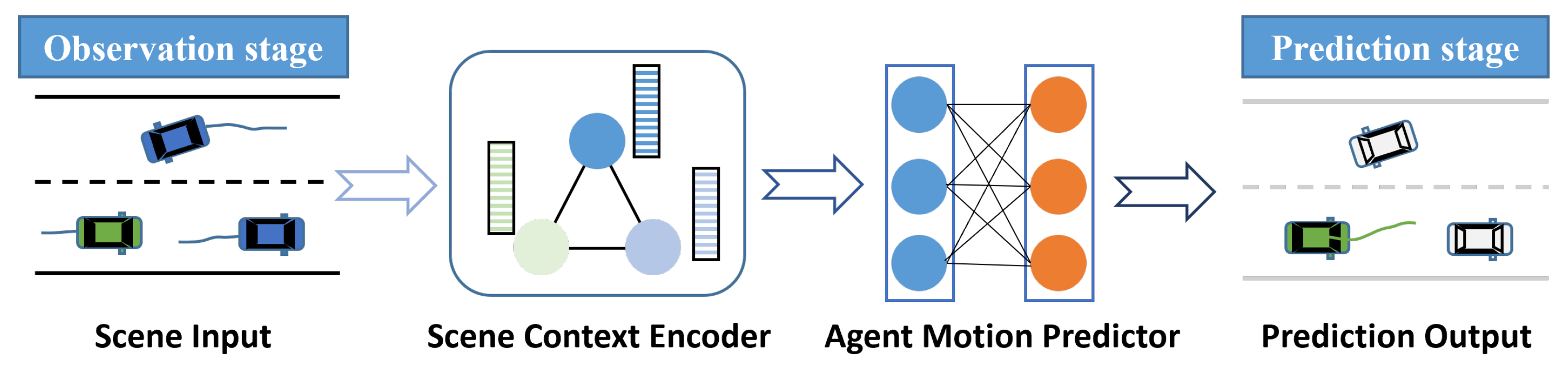
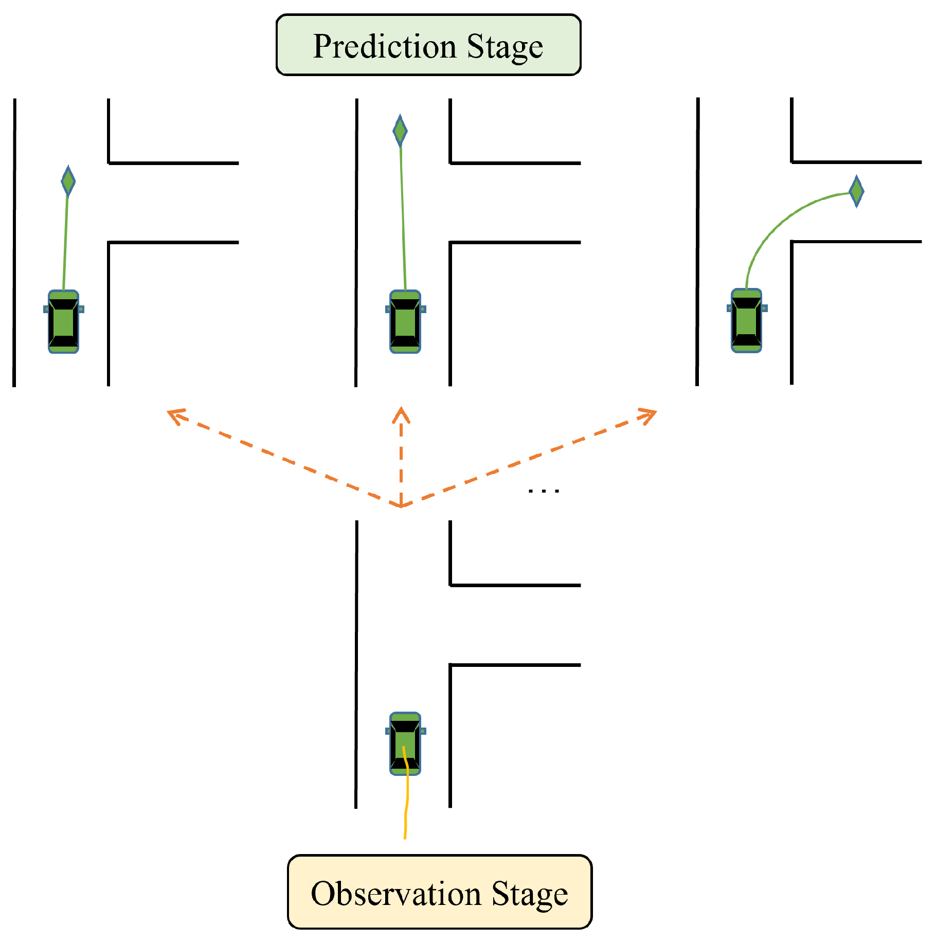
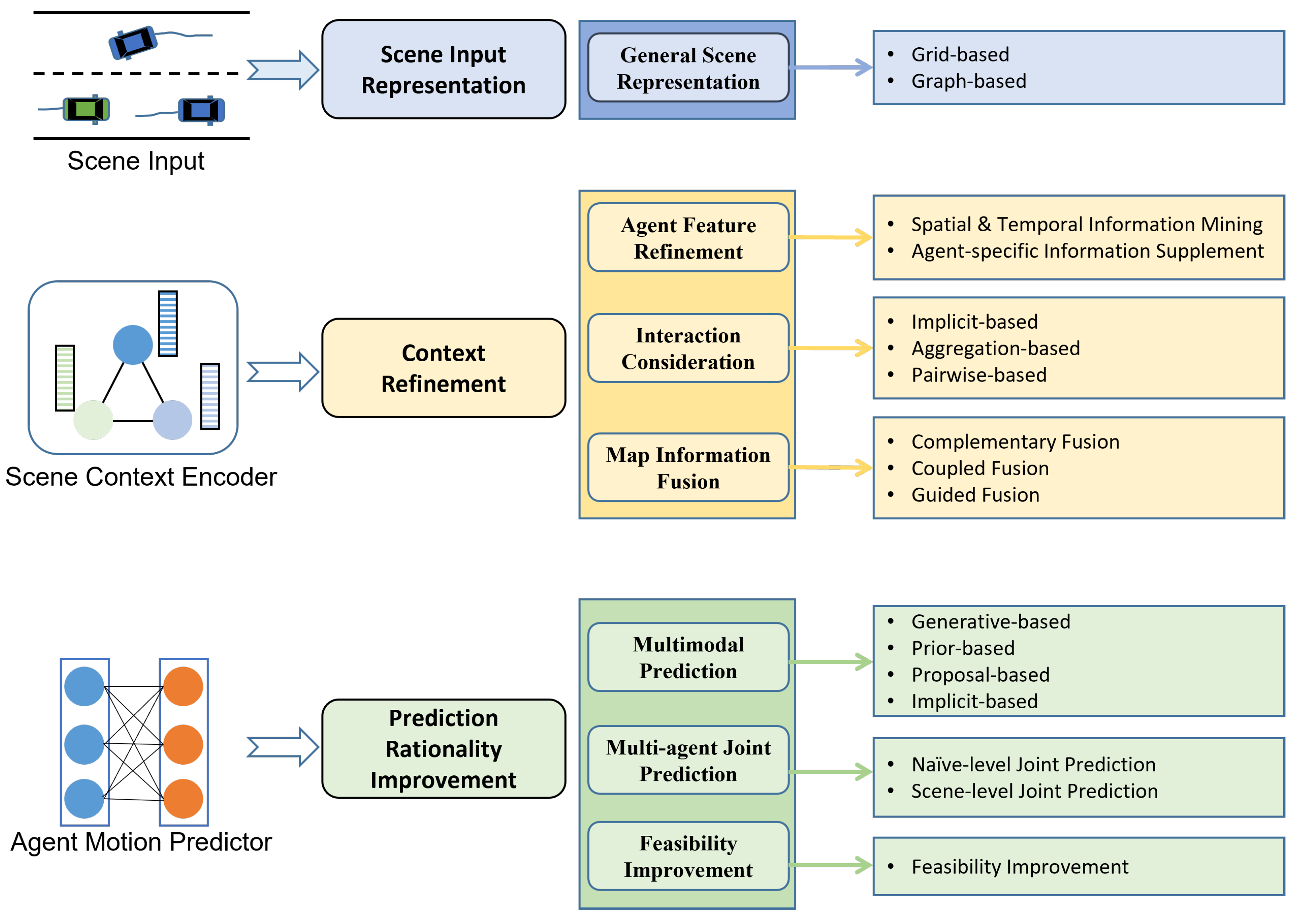
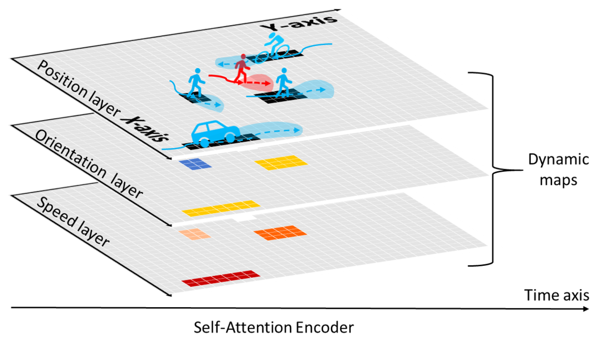
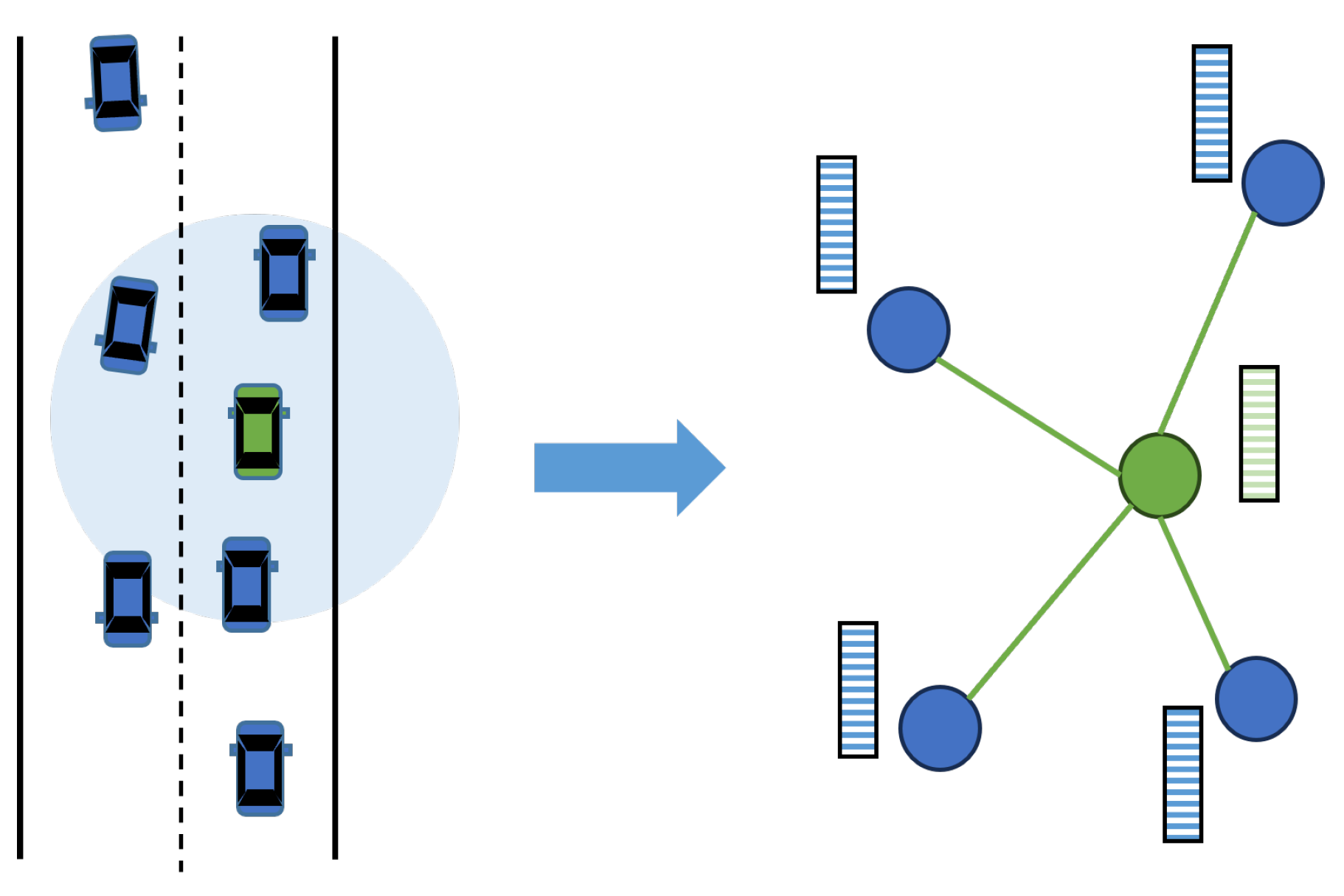
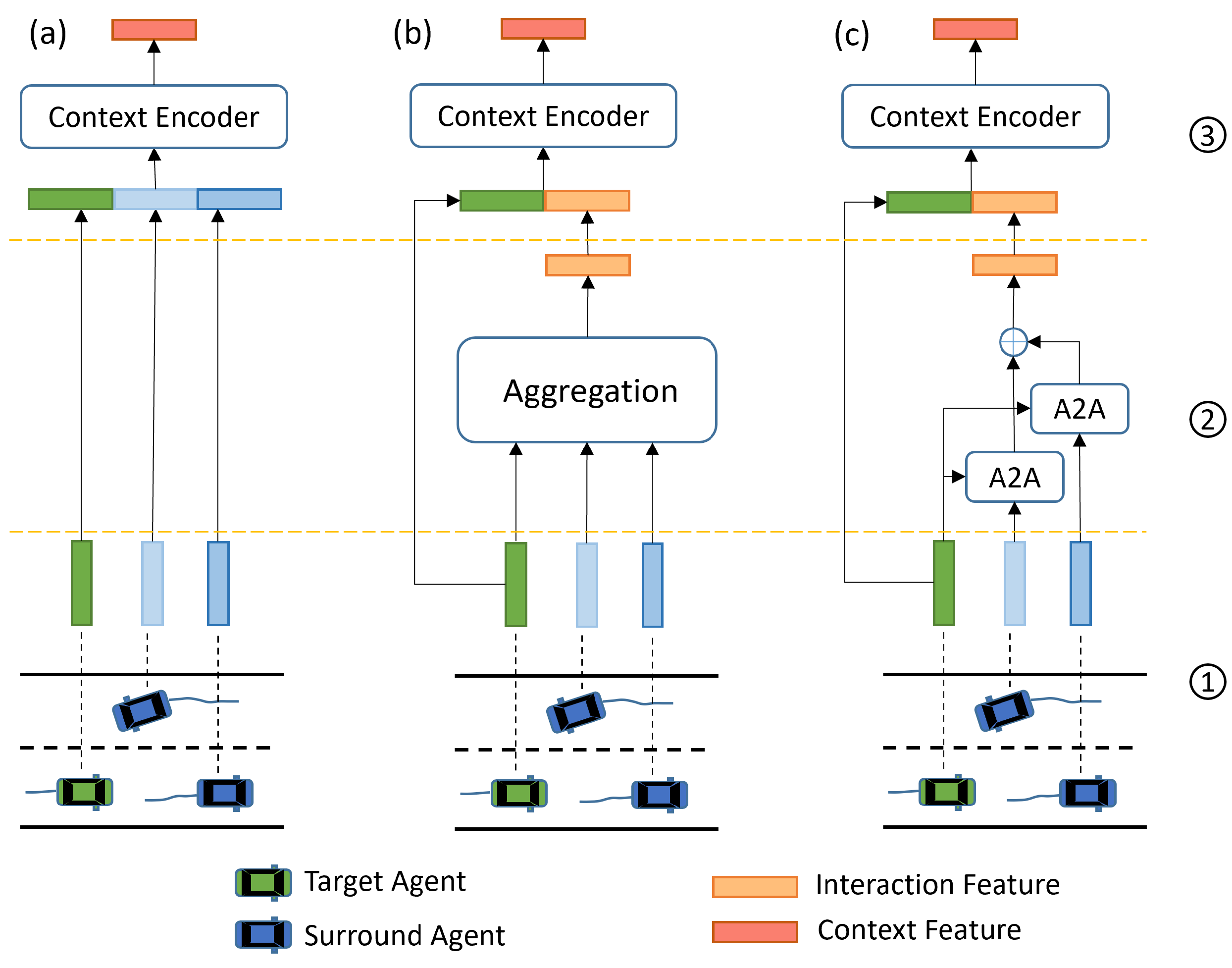
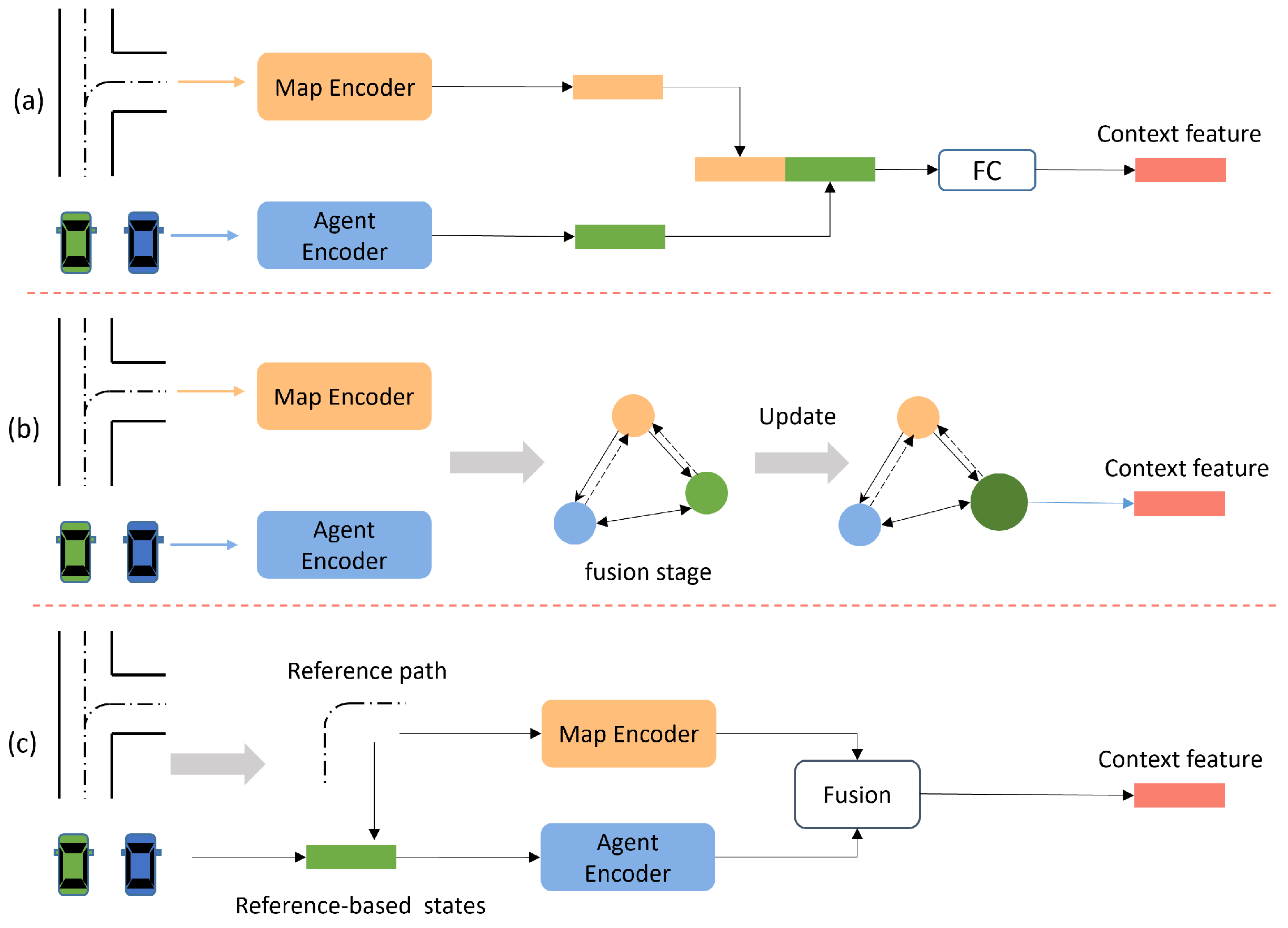
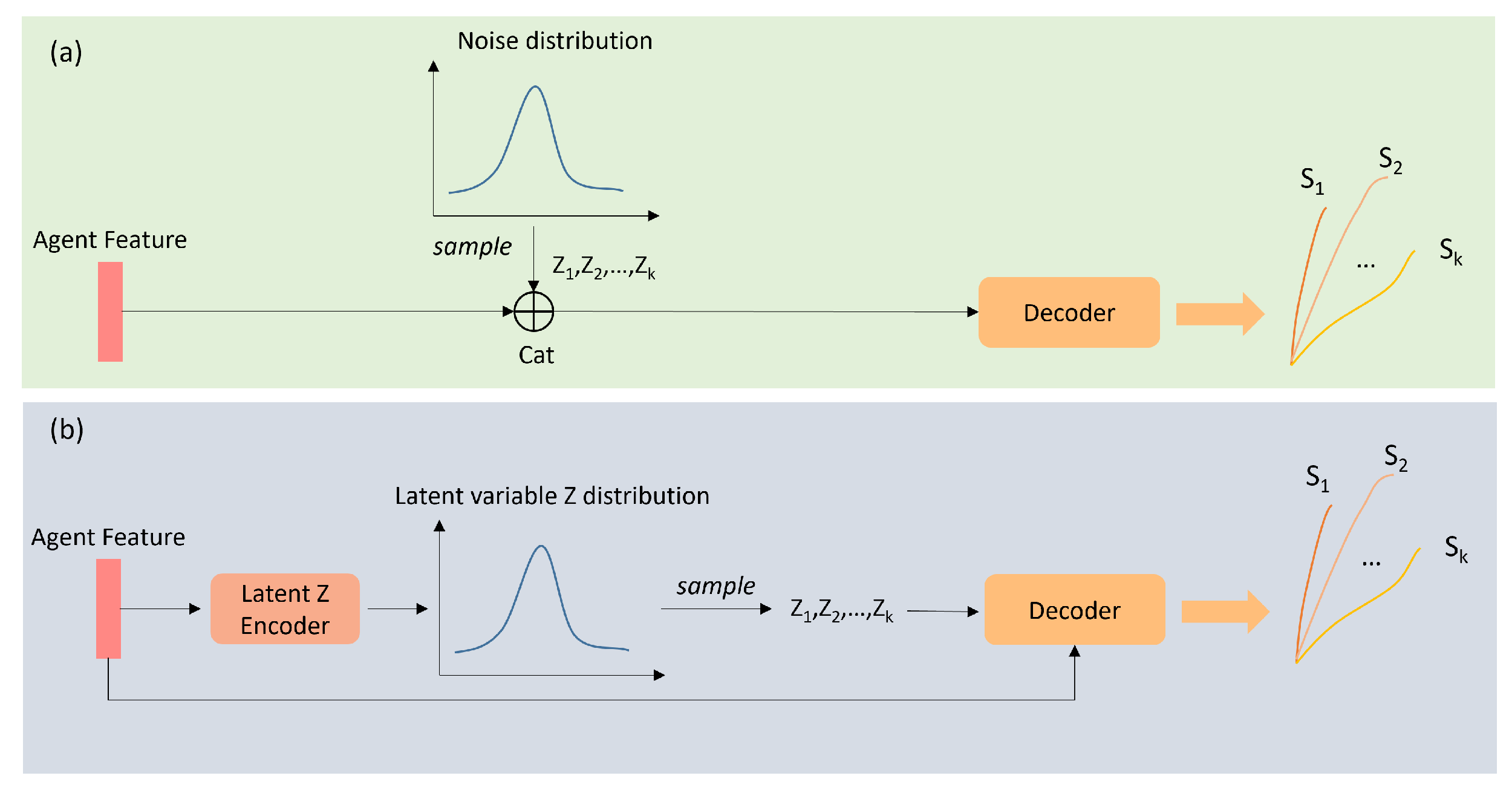
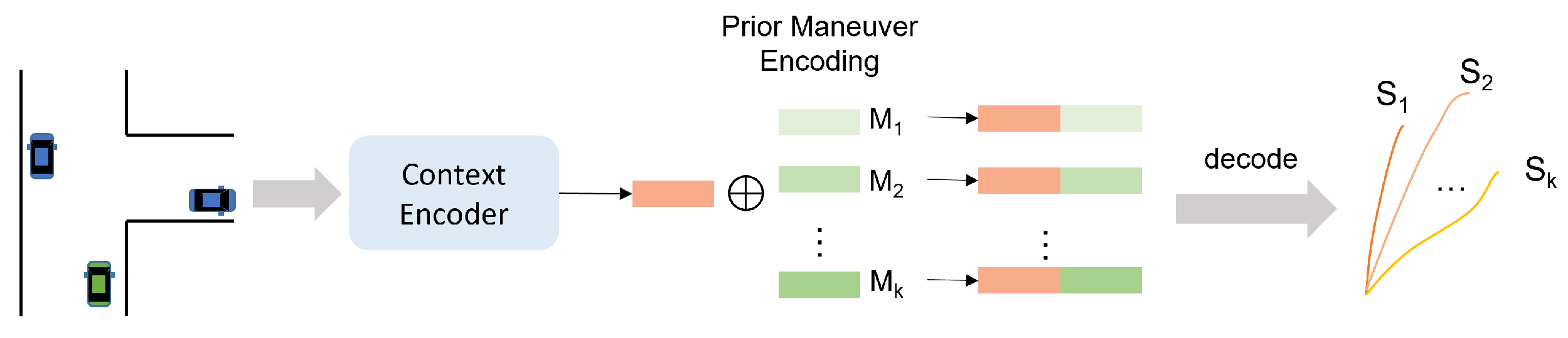

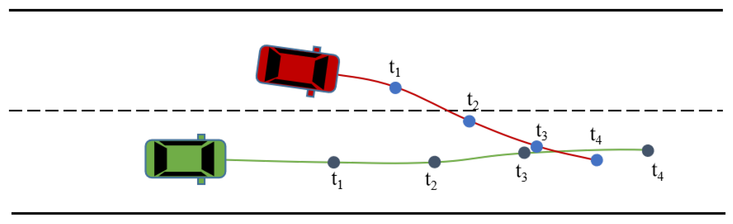
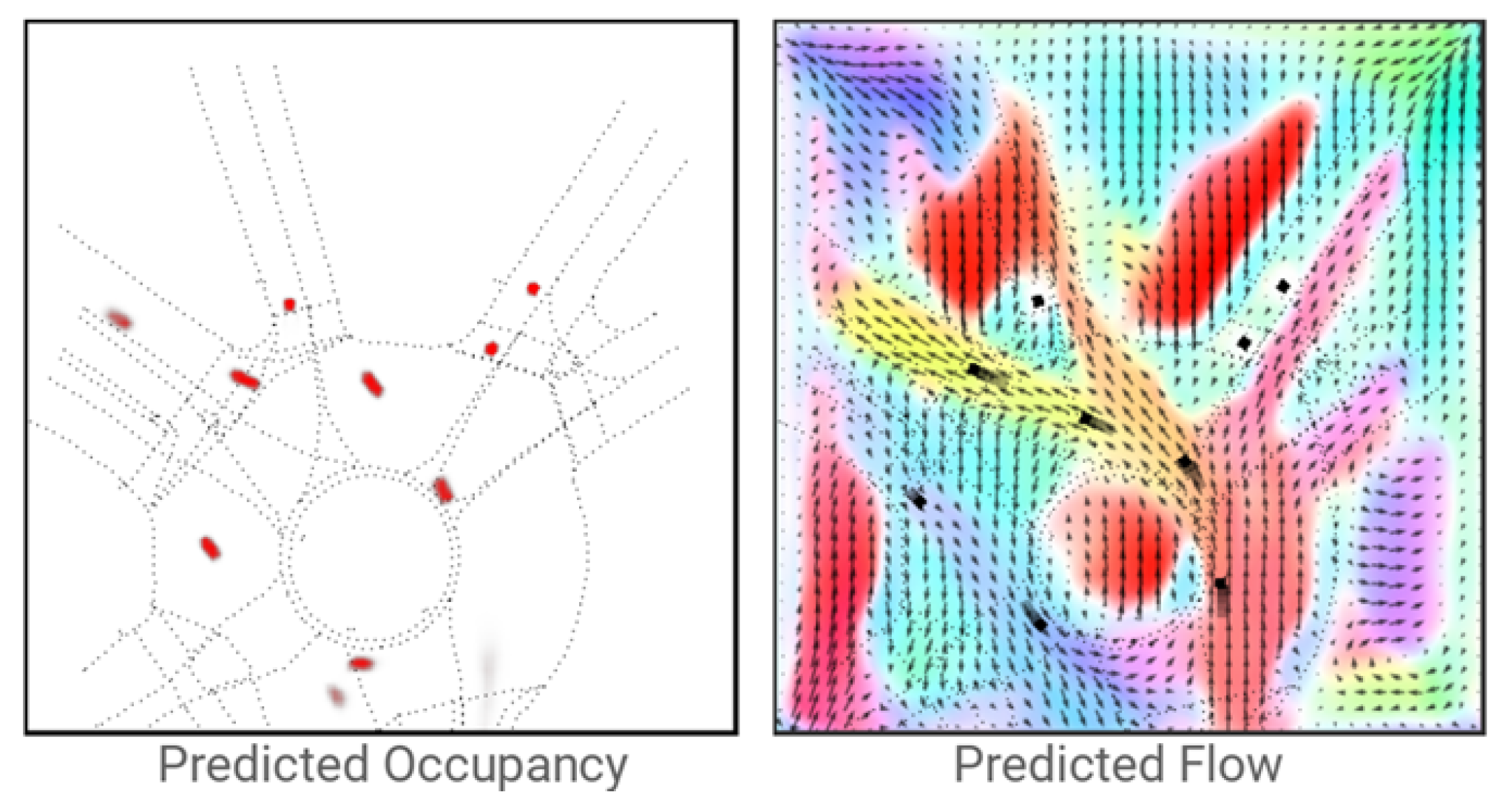
Disclaimer/Publisher’s Note: The statements, opinions and data contained in all publications are solely those of the individual author(s) and contributor(s) and not of MDPI and/or the editor(s). MDPI and/or the editor(s) disclaim responsibility for any injury to people or property resulting from any ideas, methods, instructions or products referred to in the content. |
© 2023 by the authors. Licensee MDPI, Basel, Switzerland. This article is an open access article distributed under the terms and conditions of the Creative Commons Attribution (CC BY) license (https://creativecommons.org/licenses/by/4.0/).