Abstract
Load forecasting has significant implications on optimizing the operation of air conditioning systems for industrial mushroom houses and energy saving. This research paper presents a novel approach for short-term load forecasting in mushroom houses, which face challenges in accurately modeling cold and heat loads due to the complex interplay of various factors, including climatic conditions, mushroom growth, and equipment operation. The proposed method combines empirical wavelet transform (EWT), hybrid autoregressive integrated moving average (ARIMA), convolutional neural network (CNN), and bi-directional long short-term memory (BiLSTM) with an attention mechanism (CNN-BiLSTM-Attention) to address these challenges. The first step of this method was to select input features via the Boruta algorithm. Then, the EWT method was used to decompose the load data of mushroom houses into four modal components. Subsequently, the Lempel–Ziv method was introduced to classify the modal components into high-frequency and low-frequency classes. CNN-BiLSTM-Attention and ARIMA prediction models were constructed for these two classes, respectively. Finally, the predictions from both classes were combined and reconstructed to obtain the final load forecasting value. The experimental results show that the Boruta algorithm selects key influential feature factors effectively. Compared to the Spearman and Pearson correlation coefficient methods, the mean absolute error (MAE) of the prediction results is reduced by 14.72% and 3.75%, respectively. Compared to the ensemble empirical mode decomposition (EEMD) method, the EWT method can reduce the decomposition reconstruction error by an order of magnitude of , effectively improving the accuracy of the prediction model. The proposed model in this paper exhibits significant advantages in prediction performance compared to the single neural network model, with the MAE, root mean square error (RMSE), and mean absolute percentage error (MAPE) of the prediction results reduced by 31.06%, 26.52%, and 39.27%, respectively.
1. Introduction
According to statistics, energy costs account for 20% to 30% of the total production costs in the industrialized production of edible mushrooms [1]. Among those costs, the air conditioning systems used to regulate the temperature in mushroom houses account for approximately 40% of the total energy cost [2]. It is expected that with the increasing proportion of industrialized production in the edible mushroom industry in China [3], the energy consumption will continue to rise. Therefore, efficient energy saving and sustainable mushroom house buildings are the direction for industry development. Researchers have proposed improvements from energy-saving and environmentally friendly enclosure structures, green energy utilization, high-efficiency air conditioning equipment, etc. Among them, intelligent control methods are one of the highly valuable and widely applicable sustainable measures for reducing energy consumption [4]. However, uncertainties, such as weather and human factors, result in significant randomness in mushroom house energy consumption. Therefore, accurate load forecasting for mushroom houses is crucial for decision making and control of air conditioning systems.
The air conditioning load forecasting methods can be mainly divided into white-box models, grey-box models, and black-box models based on their forecasting principles [5]. White-box models are difficult to establish due to the challenges in modeling accuracy. These models involve a significant quantity of parameters, such as the thermal capacitance and thermal conductivity of various components. Additionally, the thermal parameters of mushroom substrates must be considered, for which it is difficult to obtain precise measurements. Simple grey-box models like the RC model are widely used in model predictive control (MPC). Their advantage lies in the ability to identify parameters with limited data and their reliability compared to black-box models, thanks to the constraints imposed by physical rules. However, as the available data increase, these models face performance limitations [6]. Research has shown that MPC methods using black-box models can achieve energy savings of 8.4%, higher than the energy savings of 7.4% for white-box models and 7.2% for grey-box models [7].
With the development of Internet of Things (IoT) technology, the cost of acquiring a large amount of real-time data has been significantly reduced. In this context, data-driven prediction methods have gained widespread attention from scholars domestically and abroad. Data-driven prediction models can be divided into statistical models represented by autoregressive (AR) models [8], autoregressive integrated moving average (ARIMA) models [9], and machine learning models represented by support vector machines (SVMs) [10], artificial neural networks (ANNs) [11], random forests (RFs) [12], support vector regression (SVR) [13], and deep learning models represented by long- and short-term memory (LSTM), gated recurrent unit (GRU), bi-directional LSTM (BiLSTM), etc.
In machine learning, Wang et al. [14] combined ANN and ensemble methods for the short-term prediction of building loads. Compared with a single ANN model, the prediction error was reduced by 24%. Yong et al. [15] used the RF method for building energy consumption prediction, and the RF model had a 10% and 6% increase in the coefficient of determination R2 compared with backpropagation neural network–ANN (BPNN-ANN) and SVM, respectively. Ahmad et al. [16] predicted the short-term, medium-term, and long-term energy consumption of building environments using a binary decision tree (BDT), compact regression Gaussian process model (CRGPM), and other methods. Dai et al. [17] improved the prediction method of SVM by optimizing it using an improved particle swarm optimization algorithm (PSO). The results showed that the mean absolute percentage error (MAPE) of the SVM prediction with an improved PSO optimization algorithm was 0.0412%, which was better than that of minimal redundancy maximal relevance–genetic algorithm–SVM (mRMR-GA-SVM), BPNN, and mRMR-BPNN, which were 0.0493%, 0.0447%, and 0.0438%, respectively. This indicates that optimizing the parameters in the prediction model through optimization algorithms can significantly improve the model’s prediction accuracy.
In deep learning, Olu-Ajayi et al. [18] compared nine algorithms, including RF, SVM, and linear regression, for predicting annual average energy consumption. They found that the deep neural network (DNN) achieved an R2 of 0.95 and a root mean square error (RMSE) of 1.16 kWh/m2, outperforming other models. Zhou et al. [19] predicted air conditioning electricity consumption using LSTM and BPNN. The results showed that compared to BPNN, LSTM reduced the MAPE of daily electricity consumption by 49% and the MAPE of hourly electricity consumption by 36.61%. Bohara et al. [20] applied BiLSTM for short-term load forecasting in residential buildings. The results showed that compared to the LSTM model, BiLSTM reduced the RMSE by 5.06%. As an improved network of LSTM, BiLSTM can handle more complex long-term sequences, extract information from both directions in the sequence, and better capture bidirectional temporal features.
To further improve the prediction accuracy, some researchers have proposed combining different algorithm models [21]. For example, Song et al. [22] proposed a combination model based on a hybrid convolutional neural network (CNN) and LSTM for predicting hourly loads in heating substations. In this model, CNN effectively extracted spatial feature matrices of the load and influencing factors, while LSTM captured the temporal features of the load. The results showed that compared to SVM, random forest regression (RFR), multilayer perceptron (MLP), and gradient-boosting regression (GBR), the RMSE of load prediction at the heating substations decreased by 0.235 GJ, 0.244 GJ, 0.237 GJ, and 0.236 GJ, respectively. The attention mechanism, which simulates the human brain’s resource allocation, has been widely applied in time-series forecasting due to its ability to enhance the weights of key influencing factors. Chitalia et al. [23] studied the attention model of recurrent neural networks (RNNs) in buildings, such as laboratories, offices, and schools. The model’s predictive performance improved by 45% compared to ARIMA, RNN, and CNN. Wan et al. [24] combined CNN, LSTM, and attention mechanism for power prediction in two units. Compared to LSTM and CNN-LSTM models, the CNN-LSTM-attention model achieved higher prediction accuracy by 1.815 MW and 1.57 MW, and 0.066 MW and 0.026 MW, respectively, outperforming single models and models without an attention mechanism. He et al. [25] proposed a hybrid prediction model combining CNN, GRU, and an attention mechanism. The results showed that compared to LSTM, the RMSE of the prediction results decreased by 1.38%, and the R2 improved by 1.49%.
Combination models can effectively improve the prediction accuracy compared to single models. However, relying solely on the performance of algorithms has limited effectiveness in improving prediction accuracy. Load data show characteristics, such as volatility, dynamics, and complexity, including trends, seasonality, noise, etc. [26]. In particular, this applies to ultra-short-term load forecasting, which refers to load forecasting within one hour [27]. Very-short-term load forecasting (VSTLF) is beneficial for optimizing the operation of energy systems [28]. The speed and accuracy of VSTLF results determine the performance of MPC for energy-saving control, and they are the prerequisite for mining energy-saving potential [29], while traditional prediction models struggle to accurately capture the inherent features in the raw data.
To solve such problems, various decomposition methods with time-series data have been proposed [30], such as wavelet transform (WT), empirical mode decomposition (EMD), ensemble empirical mode decomposition (EEMD), etc. Wang et al. [31] used WT to decompose photovoltaic power data and established deep convolutional neural networks (DCNNs) for each item of decomposed data, combined with quantile regression (QR) for prediction. The reconstructed results outperformed BPNN, SVM, etc., with an average improvement of 52.25% in RMSE and 56.64% in mean absolute error (MAE) compared to other models. Gao et al. [32] used EMD to decompose the original load data, selected decomposition sequences highly correlated with the original load through Pearson correlation analysis, and combined them with the original data sequence as inputs to the GRU network for short-term load forecasting. Compared to single models, such as GRU, SVR, RF, as well as EMD-GRU, EMD-SVR, and EMD-RF models, the proposed method achieved the best performance in terms of RMSE (1484.17 kWh) and MAPE (3.08%) for July forecasting in the M1 dataset. Mounir et al. [33] proposed a method that combines EMD and BiLSTM to achieve more accurate load forecasting. By decomposing the information on multiple time scales using EMD and capturing short-term and long-term information in each component using BiLSTM, the EMD-BiLSTM model reduced the MAE by 0.07 and the MAPE by 0.14% compared to the BiLSTM model. The introduction of EMD effectively captures complex temporal and spectral features in the data, improving the prediction accuracy. However, EMD decomposition may suffer from mode mixing and endpoint effects. To address this, He et al. [34] proposed a short-term wind power prediction method based on EEMD and the least absolute shrinkage and selection operator–quantile regression neural network (LASSO-QRNN). Compared to LASSO-QRNN without EEMD, it achieved a 60.96% reduction in MAE. However, the EEMD algorithm, which solves the mode-mixing problem by adding white noise, also introduces reconstruction errors, affecting the prediction accuracy. The EEMD decomposition algorithm, due to the multiple additions of white noise and multiple EMD decompositions, increases the computational complexity and reduces efficiency. None of the above methods analyze the characteristics of each component after decomposition to select suitable methods for better prediction.
Empirical wavelet transform (EWT), proposed by Gilles in 2013 [35], is an adaptive method that can select frequency bands, overcome mode mixing, and reduce computational complexity. It has promising applications. The accuracy of the prediction model can be effectively improved by analyzing the different characteristics of the decomposed load data and establishing the most suitable prediction model based on these characteristics [36,37].
In summary, deep learning neural network methods have been widely studied and have shown good application results in commercial buildings and power distribution. However, mushroom cultivation facilities in edible fungus factories differ from commercial buildings. The internal mushroom substrate density is high, and the indoor thermal hysteresis is significant. Moreover, the target temperature indoors needs to be changed, synchronizing with the growth cycle of the mushrooms. This article proposes a prediction method for rapidly changing the cooling and heating loads in mushroom cultivation facilities based on EWT decomposition. Firstly, the EWT method is used to decompose the load into multiple intrinsic mode functions. Then, the Lempel–Ziv algorithm is utilized to classify the modal components. The components are then reconstructed into high-frequency and low-frequency parts. Finally, the CNN-BiLSTM-attention model and the ARIMA model are used separately to predict the load. The proposed load prediction method is validated and compared with commonly used prediction methods using actual data from a mushroom factory, demonstrating its effectiveness in load prediction.
2. Materials and Methods
2.1. Data Source
The experimental site was located in a factory where the edible fungus hypsizygus marmoreus is produced, in Tongzhou District, Beijing. The length, width, and height of the experimental mushroom house were 14 m, 8 m, and 5 m, respectively. The ground of the mushroom house was formed of hardened concrete, and the surrounding walls and roof enclosures of the mushroom house were polyurethane steel plates in sandwich color with a thickness of approximately 100 mm. The mushroom house had control equipment such as fixed-frequency air conditioners, fresh air fans, exhaust fans, and humidifiers.
In order to obtain relevant data affecting the load of the mushroom house, the air temperature and humidity inside and outside the mushroom house were continuously measured using HOBO U23-001A (Onset Computer Corporation, Bourne, MA, USA), (accuracy: ±0.2 °C, ±2.5%). The working status of the air conditioner was checked and monitored via an HOBO CTV-C (Onset Computer Corporation), (accuracy: ±5 A) current collector, and the sampling intervals were set to 1 min. The fresh air velocity was measured using a Delta HD2903T wind speed sensor (Delta OHM S.r.l., Padua, Italy) (accuracy: ±3%); the CO2 concentration was measured using a Vaisala’s GMP252 sensor (Vaisala Oyj, Vantaa, Finland); the solar radiation was measured using Kipp and Zonen’s SMP3 sensor (Royal Kipp & Zonen BV, Amsterdam, The Netherland); the wall heat flux was measured using a Hukseflux HFP01 heat flux sensor (Hukseflux Thermal Sensors B.V., Amersfoort, Holland), which was connected to Campbell’s CR1000X data collector (Campbell Scientific, Inc., Logan, UT, USA) for continuous recording, and the sampling interval was 1 min.
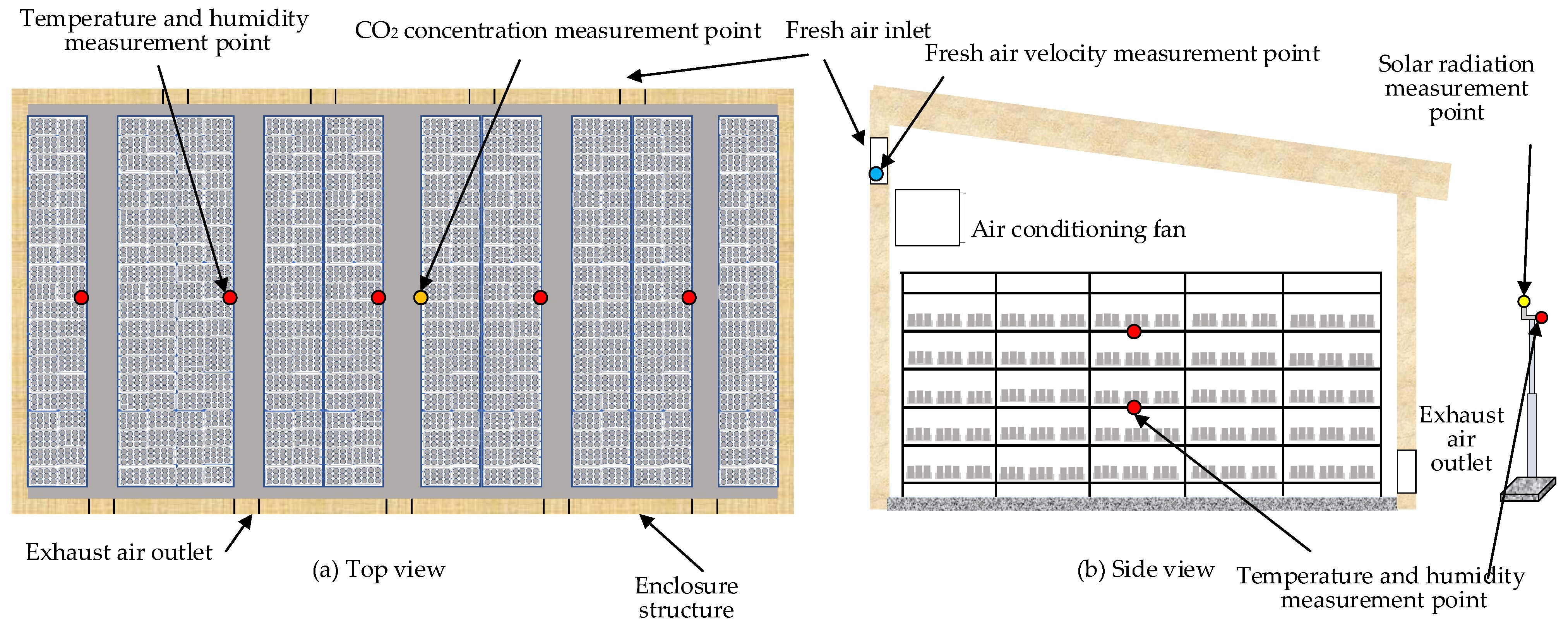
The deployment of the mushroom house measuring equipment is shown in Figure 1. The temperature and humidity sensors were evenly arranged in the middle of the mushroom house with five measurement points in the east–west direction; two layers were arranged at equal distances in the vertical direction of the cultivation shelf, with a total of ten sensors; the wind speed sensor was installed at the air inlet of the fresh air pipeline; the CO2 sensor was arranged in the center of the house; the outdoor air temperature, humidity, and solar radiation sensors were attached to a pole at a distance of 5 m from the mushroom house, with a height of 2 m. Data were collected from 11 July 2022 to 15 September 2022, totaling 729,300 data.
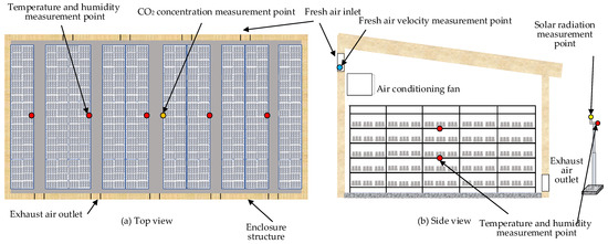
Figure 1.
Arrangement of measuring points in the mushroom house: (a) top view of the experimental mushroom chamber; (b) side view of the chamber.
2.2. Data Processing
Data processing includes three parts: outlier handling, feature filtering, and normalization, as shown in Figure 2.
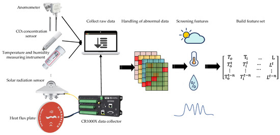
Figure 2.
Data processing.
The acquired data are graded as missing and abnormal due to the equipment itself or transmission, which affects the accuracy of the prediction model. For missing data, the front and rear data of the missing position are used to fill the gaps through linear interpolation, and the calculation method is shown in Equation (1); for abnormal data, the mean method is used for smoothing and filtering, and the calculation method is shown in Equation (2):
where is the missing data at time ; is the original data at time ; is the original data at time :
where is abnormal data; , are adjacent to the valid data.
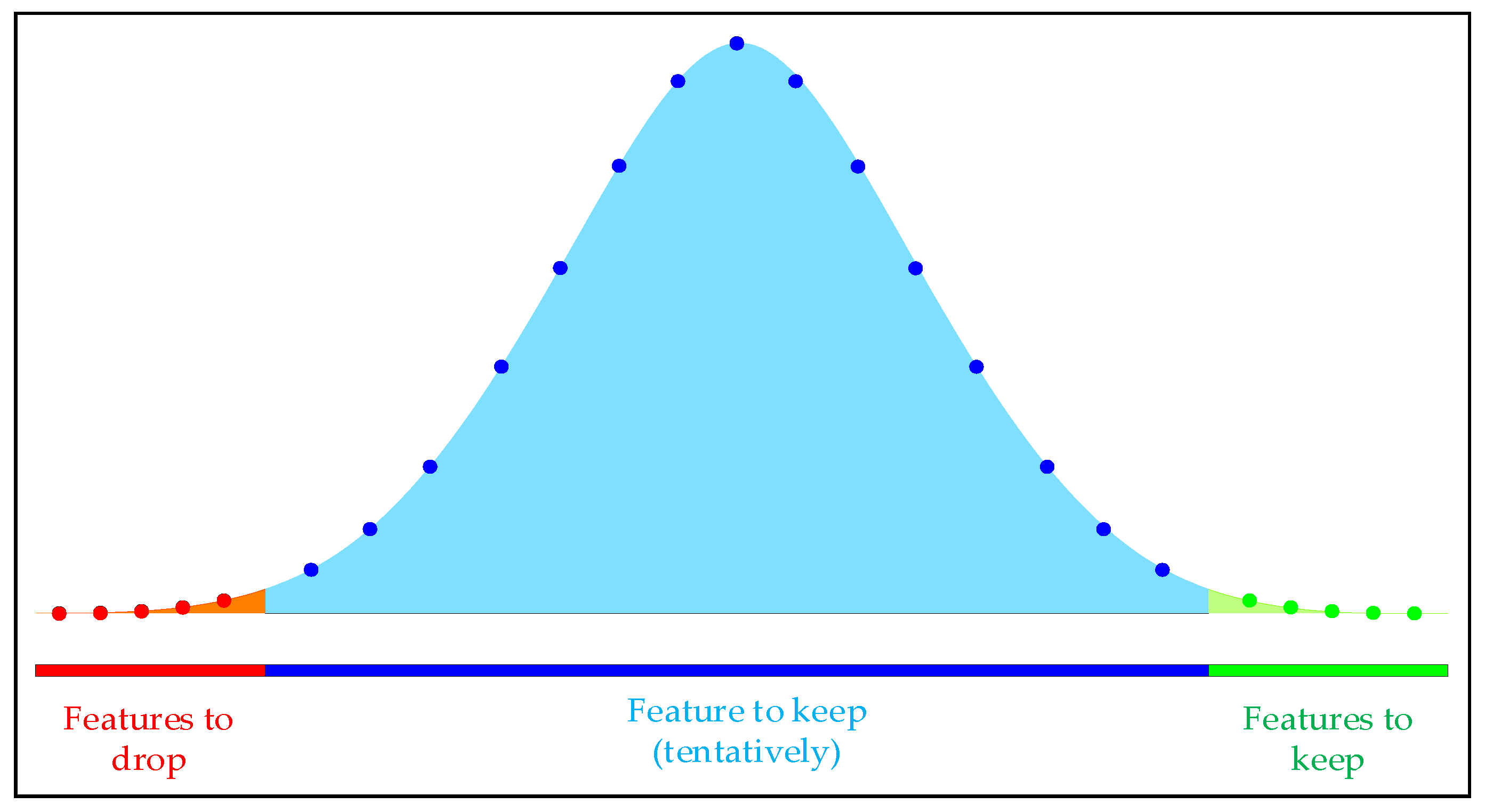
In order to improve the efficiency of model prediction, the Boruta algorithm is used to filter out key input features and construct a feature set for model training. The Boruta algorithm calculates the binomial distribution of feature selection probability through multiple iterations, as shown in Figure 3.
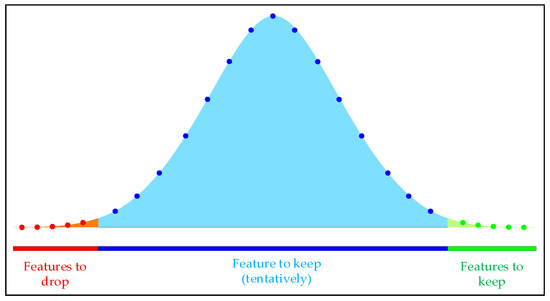
Figure 3.
Multiple experimental binomial distribution.
The red area represents the rejection region, where features falling within this area are eliminated during iteration. The blue area indicates the uncertain region, where features falling within this area remain pending throughout the iterative process and require further determination based on the selection threshold and feature importance. The green area represents the acceptance area, where features falling within this area are directly retained.
In order to eliminate the influence of the load parameters of the mushroom house on the training of the neural network prediction model due to the difference between the dimensions, it is necessary to normalize all factors, and the calculation method is shown in Equation (3):
where is the maximum value; is the minimum value; and is the normalized value.
2.3. Model Experimental Environment
The computer configuration of the experimental platform is as follows: equipped with AMD Ryzen (TM) 7 5800H CPU (Advanced Micro Devices, Inc., Santa Clara, CA, USA), NVIDIA GeForce GTX 1650 4G GPU (NVIDIA Corporation, Santa Clara, CA, USA), 16 GB of memory, and 64-bit Windows 10 operating system. The software uses Keras-2.9 as a deep learning tool, Tensorflow-gpu-2.3 as a deep learning framework, the programming language is Python, the Python version is 3.7, and the integrated development environment is Visual Studio Code.
2.4. Model Prediction Evaluation Indicators
In order to quantitatively evaluate the effect and accuracy of the model’s prediction, this paper uses RMSE, MAE, MAPE, and R2 as indicators to measure the prediction accuracy. The calculation methods of RMSE, MAE, MAPE, and R2 are shown in Equations (4)–(7):
where is the actual values; is the predicted values; is the mean of the actual value; and is the total amount of data.
2.5. Process Design
The model prediction process proposed in this article is shown in Figure 4; the specific steps are as follows:
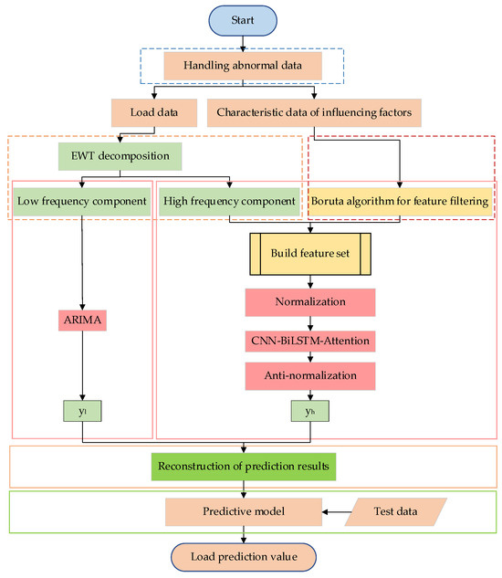
Figure 4.
Model prediction flow.
- Exception data processing: Missing and abnormal values in the collected data were processed using interpolation and smoothing filter methods, respectively, to obtain a complete dataset;
- Load data decomposition: The EWT method was used to decompose the load of the mushroom house into modal components of different scales. The Lempel–Ziv method was then applied to classify the modal components into high-frequency and low-frequency categories, reconstructing all components into high-frequency and low-frequency feature components;
- High-frequency feature selection: The Boruta algorithm was used to determine the input features of the neural network model. An input feature set was constructed, and the dataset was divided into training, validation, and testing sets in a ratio of 7:2:1;
- Predictive model construction: For the high-frequency feature components, the dataset in Step 3 was first normalized, and then the CNN-BiLSTM-Attention model was used to predict; the high-frequency feature prediction results were obtained after inverse normalization. For the low-frequency feature components, an ARIMA prediction model was established to address the drawback of the neural network being less insensitive to linear features. Finally, the results from the high-frequency and low-frequency prediction models were combined and reconstructed to obtain the final result;
- Model prediction: Based on the test data and the prediction values from the model, model error metrics were obtained to evaluate the model’s prediction performance.
2.6. Predictive Model Structure
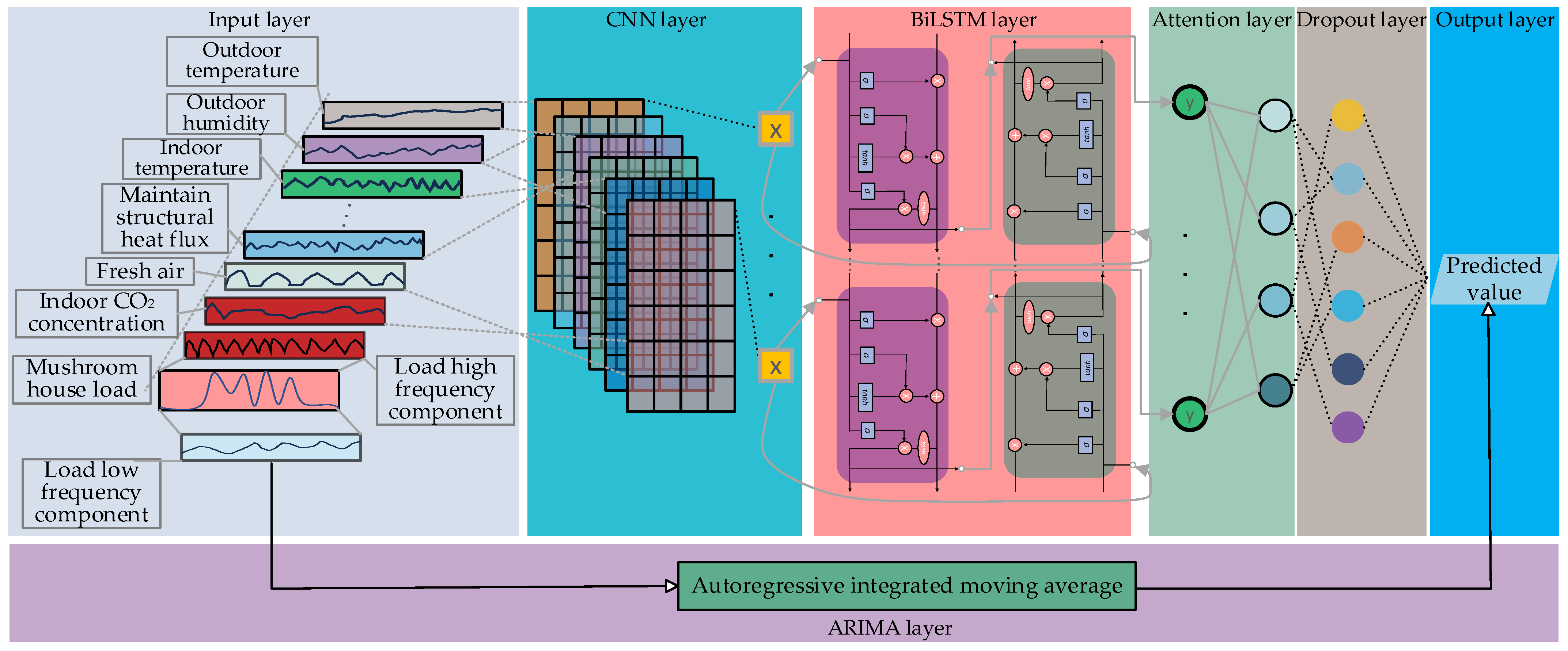
The overall structure of the hybrid ARIMA and CNN-BiLSTM-attention model proposed in this paper is shown in Figure 5.

Figure 5.
Combined model structure of ARIMA and CNN-BiLSTM-attention.
Input layer: For the high-frequency part of the load, the input features are filtered using the Boruta method to establish key feature vectors, and then the historical 4-h load data are used to predict the load changes in the next 10 min, and the input features with data dimension (24, 7) are constructed and input to the CNN layer; for the low-frequency part of the load, it is directly entered into the ARIMA model.
CNN layer: Extract the input feature matrix information by setting the two-layer CNN layer. After passing through the first layer, the data dimension becomes (24, 7, 15); through the pooling layer pooling, the data dimension is transformed into (24, 3, 15), and then input to the second layer convolution layer. The data dimension is transformed into (24, 3, 1), then a single layer Squeeze layer is added, the data dimension to (24, 3) and input to the BiLSTM layer. The above process activation functions all use the ReLU function.
BiLSTM layer: Set the BiLSTM layer as a single layer, and the activation function is Tanh. After passing through the BiLSTM layer, the data dimension becomes (24, 128).
Attention layer: Due to the different degrees of influence of various influencing factors on the load in the time series, an attention mechanism is introduced, and the calculation process is shown in Equations (8) and (9):
where, K, V, and Q represent Key, Value, and Query; the dimensions are all (24, 128); F (Q, K) represent the similarity between Query and Key and are calculated using the dot product method of Query and Key [38].
ARIMA layer: The ADF unit root method detects whether the low-frequency load part is a non-stationary sequence. After a differential transformation, it is a stationary sequence and input to the ARIMA layer. The p, d, and q are 2, 1, and 1, respectively.
Output layer: Add the dropout layer before the output layer to inactivate the neurons (the inactivation rate is 0.1) to prevent overfitting of the high-frequency part. After inactivation, the data dimension is (32), and then through reconnecting to a fully connected layer and obtaining the high-frequency load prediction result , the low-frequency load prediction result is obtained through the ARIAM layer. Subsequently, the two results are combined to obtain the final load prediction value.
3. Results
3.1. Analysis of Feature Set Construction Method
The original data consist of nine input features and are divided into three categories: outdoor climatic factors, indoor environmental factors, and equipment working status, as shown in Table 1.

Table 1.
Characteristics of the collected data.
The Boruta algorithm was applied to screen the input features mentioned above, with 80 iterations being set for the Boruta algorithm. The iteration process is shown in Table 2. Through Boruta algorithm screening, the algorithm stopped at the 38th iteration, during which two input features were rejected and seven input features were accepted. The accepted features include outdoor temperature, outdoor humidity, heat flux, indoor temperature, indoor CO2 concentration, the fresh air volume, and air conditioning opening time.
Table 2.
Iterative process of feature screening for the Boruta algorithm.
In order to verify the performance of the Boruta method in feature selection, the constructed prediction model was used to validate the performance of the Boruta algorithm, the Pearson correlation coefficient method, and the Spearman correlation coefficient method, with the original data as the control. The results are shown in Table 3.
Table 3.
Results of different feature screening methods.
According to Table 3, the model prediction performance was best after feature screening via the Boruta algorithm. The MAE was 0.591 kW, which was reduced by 16.88%, 14.72%, and 3.75% compared to the control group, the Spearman correlation coefficient method, and the Pearson correlation coefficient method, respectively. The RMSE was 1.056 kW, which was reduced by 18.20%, 16.52%, and 13.30% compared to the control group, the Spearman correlation coefficient method, and the Pearson correlation coefficient method, respectively. The MAPE was 5.68%, which was reduced by 16.10%, 12.74%, and 5.80% compared to the control group, the Spearman correlation analysis, and the Pearson correlation analysis, respectively. This was because the Boruta algorithm rejected indoor humidity and solar radiation, the Spearman correlation coefficient method (discriminant coefficient ≥ 0.2) removed indoor humidity, and the Pearson correlation coefficient method (discriminant coefficient ≥ 0.2) screened out indoor humidity, solar radiation, and indoor CO2 concentration. Moreover, the solar radiation data were distorted due to tree shading, and the building heat flux more accurately reflected the impact of solar radiation on the load of the mushroom house. The CO2 concentration reflected the heat production of mushrooms during non-ventilation periods, and its removal in the Pearson correlation coefficient method contradicted physical rules [39,40]. Additionally, the Boruta algorithm had a training time that was 2 s shorter than that of the Spearman and the Pearson correlation coefficient methods. Therefore, the Boruta algorithm identified the optimal input feature set and improved the computational efficiency of the prediction model.
3.2. Analysis of EWT Decomposition and Reconstruction Results of Load Data
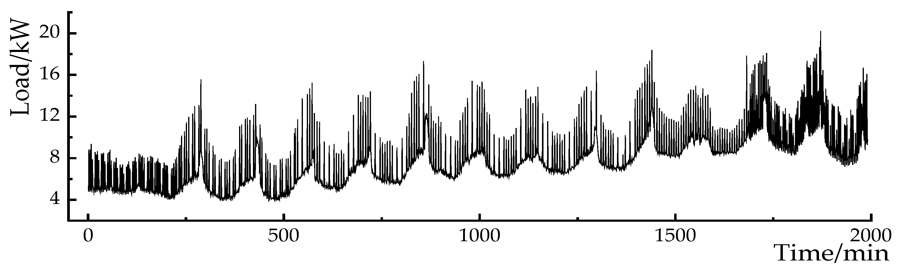
In order to effectively separate the information mixed in the original data, the EWT method is used to decompose the mushroom house load data into different scale components. The mushroom house load data are shown in Figure 6. The decomposition is performed at scales of 3, 4, 5, and 6, and the absolute reconstruction errors at each scale are shown in Table 4. When the decomposition scale is set to 4, the reconstruction error is the smallest, and the decomposition results are shown in Figure 7.
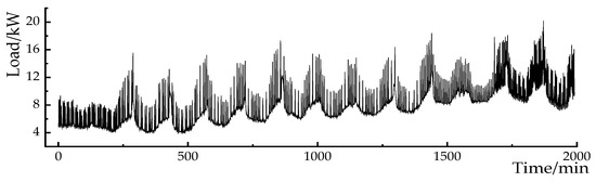
Figure 6.
Load curve of the mushroom house.
Table 4.
Sum of the absolute errors of the different decomposition components.
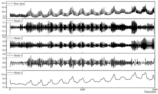
Figure 7.
Results of EWT decomposition of load data.
In order to evaluate the accuracy of the EWT algorithm and the EEMD algorithm in the load decomposition reconstruction, the reconstruction error results are shown in Figure 8. The reconstruction error of the EWT algorithm is much smaller than the reconstruction error of the EEMD algorithm. The result of the EWT reconstruction error fluctuates up and down within , and the reconstruction error of the EEMD fluctuates in a range of . The difference in reconstruction accuracy between the two algorithms is in the order of magnitude of .
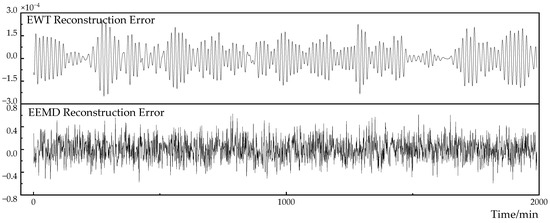
Figure 8.
Comparison of EWT and EEMD reconstruction errors.
Mounir et al. [33] used the EMD to decompose wind power data and used BiLSTM to make predictions, and the calculation amount was large. In order to improve the efficiency of the model, Yuan et al. [41] first used the EEMD algorithm to decompose the load and then used the zero-crossing rate method to determine each decomposition component. They reconstructed the load into high- and low-frequency components according to the determination results, which effectively improved the calculation efficiency of the model. However, the zero-crossing rate method only uses the number of zero-crossing axes as the criterion, which is susceptible to background noise interference and leads to misjudgment. This paper uses the Lempel–Ziv algorithm as the classification standard for eigenmode components. For high-frequency features, the complexity is higher due to repeated fluctuations in the short term; on the contrary, low-frequency features have a lower complexity due to long-term trend characteristics. The calculation process of the Lempel–Ziv algorithm is as follows:
- Calculate the complexity of each mode and denote it as , n = 1, …, N;
- Select the critical parameter (general value 0.8) to obtain the minimum value that satisfies the formula;
- Determine that 1 to m are the high-frequency components, and m + 1 to n are the low-frequency components.
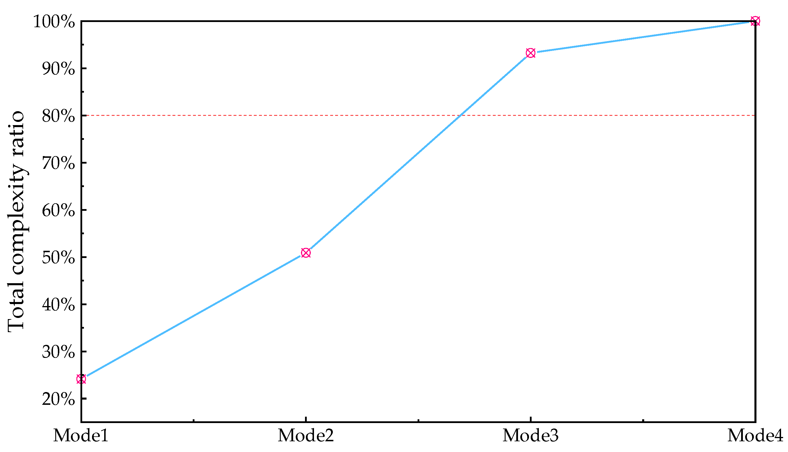
The calculation result of the cumulative complexity is shown in Figure 9.
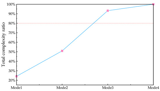
Figure 9.
Percentage of cumulative complexity for each mode.
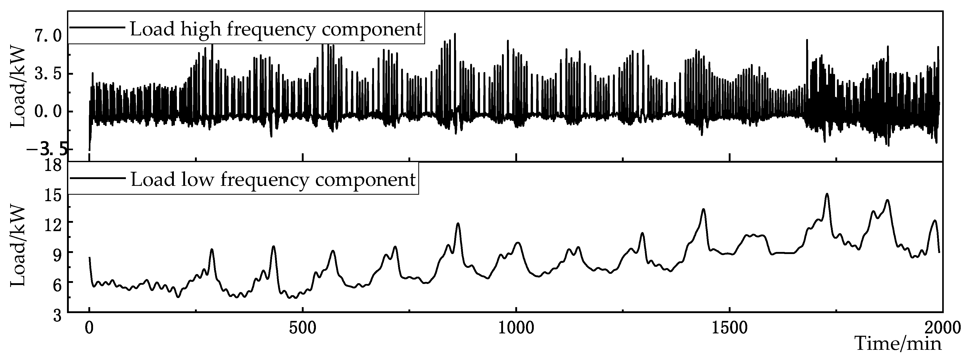
When m is 3, the proportion of cumulative complexity to total complexity exceeds the critical value. Therefore, the first- to third-mode components are selected as high-frequency feature components, and the fourth-mode component is selected as the low-frequency feature component. The mushroom house load is reconstructed according to the high and low frequencies, as shown in Figure 10.
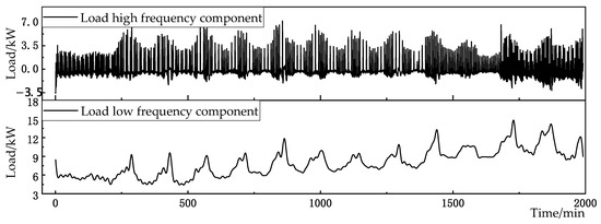
Figure 10.
EWT decomposition of load data.
3.3. Research on Neural Network Model Optimization
3.3.1. Model Hyperparameter Selection Analysis
The performance of neural network models is closely related to the setting of hyperparameters [42]. Bouktif et al. [43] optimized the LSTM hyperparameters in their prediction model using GA and PSO. This paper uses an improved non-dominant sorting genetic algorithm 2 (NSGA-II) for optimization. In order to compare the performance of PSO, GA, and NSGA-II in hyperparameter selection, the pseudocode and parameter settings for the optimization algorithm are shown in Algorithm 1 and Table 5. The number of convolutional kernels in the CNN layer and the number of neurons in the BiLSTM layer are optimized with the minimum MAE as the constraints. The optimization results and prediction errors are shown in Table 6 below.
| Algorithm 1: pseudocode for model hyperparameter optimization. | |
| Input: Convolutional kernel variable ; The variable of BiLSTM’s neurons ; The original data time series Output: The number of convolutional kernels ; The number of BiLSTM’s neurons | |
| 1 | Obtain the predicted results: = CNN-BiLSTM-Attention (,,) |
| 2 | Calculate the MAE between and label : = MAE () |
| 3 | Set parameters for NSGA-II: The number of parent population; The number of offspring population; Crossover probability; Mutation probability; Number of iterations: |
| 4 | for variable of iterations t in do |
| 5 | combine parent and offspring population: |
| 6 | F = (,,), all nondominated fronts of : F = fast-non-dominated-sort () |
| 7 | choose the first () elements of |
| 8 | use selection, crossover and mutation to create a new population create-new-pop () |
| 9 | t = t + 1 |
| 10 | Obtain and |
Table 5.
Parameterization of the NSGA-II algorithm.
Table 6.
Algorithm optimization results and model prediction errors.
As can be seen from Table 6, after using the NSGA-II algorithm to optimize the model parameters, the prediction results are significantly better than the PSO algorithm and the GA algorithm. The MAE of the NSGA-II algorithm is 0.557 kW, which is 4.46% and 2.28% lower than the PSO algorithm and the GA algorithm, respectively; its RMSE is 0.884 kW, which is 22.46% and 8.58% lower than the PSO algorithm and the GA algorithm, respectively; its MAPE is 5.26%, which is 5.90% and 3.84% lower than the PSO algorithm and the GA algorithm, respectively. The NSGA-II algorithm has better convergence and global search capabilities than the PSO and GA algorithms due to the introduction of population non-dominated sorting and diversity maintenance mechanisms, thereby improving the prediction accuracy.
Based on the above optimization results, the detailed parameters in the model are shown in Table 7.
Table 7.
Parameter settings of hybrid model.
3.3.2. Loss Function Optimization Strategy
Deep learning neural networks use mean squared error (MSE) as the default loss function, and the formula is shown in Equation (10):
where is the Frobenius norm; is the predicted sequence; is the actual sequence; and n is the total amount of data. It is susceptible to interference from discrete point data in the gradient direction update, resulting in poor model robustness. The MAE loss function maintains a constant gradient throughout the entire training process, enhancing the model’s resistance to noise interference and addressing the issue of gradient explosion during training [44]. The formula is shown in Equation (11):
where is the 1 norm. This method is prone to oscillations at the minimum value, making it difficult to converge. In order to solve the above problems, this paper adopts the segmented function as the loss function for the model, and the formula is shown in Equation (12):
The model’s prediction performance under different loss functions is shown in Table 8. By using a segmented function as the loss function for model training, with the same dataset for parameter training and prediction, the resulting MAE of the final prediction result is 0.497 kW. Compared to using MAE and MSE as the loss functions, the error is reduced by 4.05% and 10.77%, respectively, for MAE and reduced by 11.69% and 6.95%, respectively, for RMSE. The MAPE error is 4.64%, which is reduced by 9.02% and 11.795%, respectively, when compared to using MAE and MSE as the loss functions.
Table 8.
Comparison of prediction errors with different types of loss functions.
The segmented loss function combines the advantages of using MSE and MAE as loss functions. When is small, it utilizes the characteristic of the loss gradient decreasing with decreasing error to converge accurately to the minimum value and prevent oscillation near the minimum value. When is large, it uniformly descends with a fixed gradient, reducing the interference of data noise on the convergence direction of the gradient.
3.4. Comparative Analysis and Research
In order to further verify the advantages of the constructed model in load prediction, LSTM [19], GRU [32], BiLSTM [20], EMD-BiLSTM [33], CNN-LSTM [22], CNN-BiLSTM, CNN-BiLSTM-attention, and the model constructed in this article will be compared and analyzed.
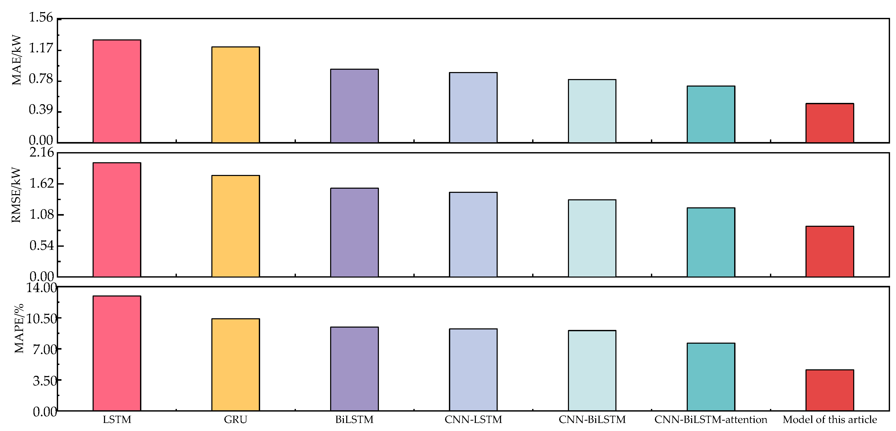
In the experimental process, the data source, pre-processing, and feature set construction methods for the above method are all the same. To avoid the influence of hyperparameters on the model in the neural network, the NSGA-II method was used to optimize it with the minimum MAE as the target. The prediction error of each model is shown in Figure 11, and the coefficient of determination R2 for the predicted results of each model is shown in Figure 12. In Figure 12, the load is divided into two categories: low and high. The low load represents the mushroom house load when the fresh air system is not activated; meanwhile, the high load represents the mushroom house load when the fresh air system is activated. The proposed model in this paper not only performs well under low-load conditions without a fresh air supply but also has better prediction capabilities for high-load conditions caused by the sudden increase in load due to the activation of the fresh air system.
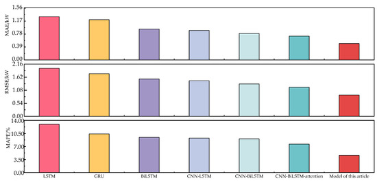
Figure 11.
Comparison of errors in prediction results between single and hybrid models.
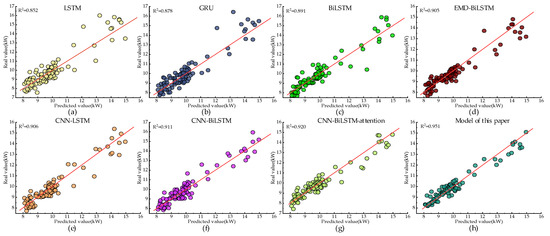
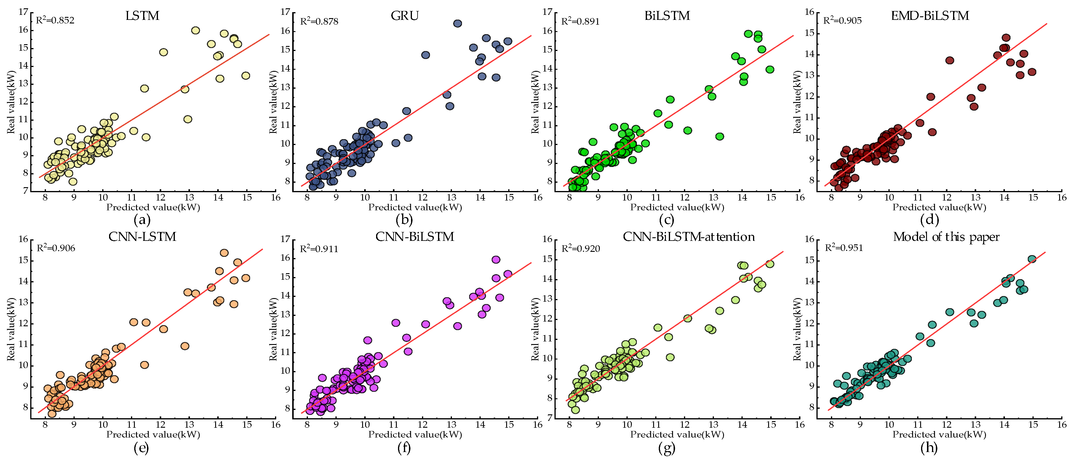
Figure 12.
The determinant coefficient R2 of the prediction results of each model: (a) The determination coefficient R2 for LSTM model’s prediction results; (b) The determination coefficient R2 for GRU model’s prediction results; (c) The determination coefficient R2 for BiLSTM model’s prediction results; (d) The determination coefficient R2 for EMD-BiLSTM model’s prediction results; (e) The determination coefficient R2 for CNN-LSTM model’s prediction results; (f) The determination coefficient R2 for CNN-BiLSTM model’s prediction results; (g) The determination coefficient R2 for CNN-BiLSTM-attention model’s prediction results; (h) The determination coefficient R2 for model of this paper’s prediction results.
Furthermore, considering Figure 11 and Figure 12a–c, it can be observed that compared to the LSTM model, the BiLSTM model decreased the MAE, RMSE, and MAPE by 28.53%, 22.35%, and 26.92%, respectively, while the R2 value increased by 4.58%. Compared to the GRU model, the BiLSTM model decreased the MAE, RMSE, and MAPE by 23.36%, 12.53%, and 8.84%, respectively, and the R2 was better than GRU’s obtained figure of 0.878. This indicates that the introduction of BiLSTM, which can extract information bidirectionally from the sequence, significantly improved the predictive accuracy of the model.
From Figure 11 and Figure 12a,c,e,f, it can be observed that compared to the LSTM model, the CNN-LSTM model decreased the MAE, RMSE, and MAPE by 31.83%, 25.92%, and 28.59%, respectively, and the R2 value of CNN-LSTM increased by 6.34%. Compared to the BiLSTM model, the CNN-BiLSTM model decreased the MAE, RMSE, and MAPE by 14.06%, 13.09%, and 4.29%, respectively, along with a 2.24% increase in R2. This is because the convolution layer can better extract local information features, thereby improving the model’s prediction accuracy.
According to Figure 11 and Figure 12f,g, it can be observed that compared to the CNN-BiLSTM model, the CNN-BiLSTM-attention model shows a decrease of 9.99% in MAE, 10.29% in RMSE, and 15.58% in MAPE, while the R2 value of CNN-BiLSTM-attention increases by 0.989%. This indicates that introducing the attention mechanism can effectively highlight important feature weights and improve the prediction accuracy.
From Figure 11 and Figure 12c,d, it can be observed that compared to BiLSTM, the EMD-BiLSTM model shows a decrease of 3.11%, 1.88%, and 1.67% in MAE, RMSE, and MAPE, respectively. Additionally, the R2 of EMD-BiLSTM is improved by 1.57%. This indicates that the model can better capture the inherent feature information in the load and improve prediction accuracy by introducing load decomposition.
From Figure 11 and Figure 12g,h, it can be observed that compared to CNN-BiLSTM-attention, the proposed hybrid ARIMA and CNN-BiLSTM-attention prediction model based on EWT decomposition decreased the MAE, RMSE, and MAPE by 31.06%, 26.52%, and 39.27%, respectively, and the R2 is 0.951, better than all other comparative models. This shows that using EWT decomposition can effectively separate the feature information in the mushroom house load, and selecting the ARIMA model and the CNN-BiLSTM-attention model for high- and low-frequency components, respectively, can effectively improve the prediction accuracy.
4. Conclusions
- (1)
- Regarding the selection of input features for prediction models, the Boruta algorithm was proposed. Compared to the control group, the Spearman correlation coefficient method, and the Pearson correlation coefficient method, the MAE of the prediction results was reduced by 16.88%, 14.72%, and 3.75%, respectively, while the RMSE was reduced by 18.20%, 16.52%, and 13.30%, respectively, and the MAPE was reduced by 16.10%, 12.74%, and 5.80%, respectively. Moreover, after using the Boruta algorithm to select features, the training time of the model was reduced by 2 s compared to methods such as Spearman.
- (2)
- The mushroom house load data were decomposed into four modal components using the EWT method, the Lempel–Ziv method was introduced to divide the modal components into high-frequency and low-frequency categories, and, finally, the same types of components were reconstructed. The experiment showed that compared to the EEMD method, the reconstruction error of the EWT method decreased from to , significantly improving the reconstruction accuracy.
- (3)
- For the high-frequency and low-frequency components of the mushroom house load, CNN-BiLSTM-attention and ARIMA prediction models were constructed, respectively. The results showed that compared to the model without feature decomposition, the MAE, RMSE, and MAP decreased by 31.06%, 26.52%, and 39.27%, respectively.
- (4)
- The NSGA-II method was used to optimize the hyperparameters of the model. Compared to the PSO and GA optimization algorithms, the MAE of the model’s prediction results decreased by 4.46% and 2.28%, respectively. The RMSE decreased by 22.46% and 8.58%, respectively, and the MAPE decreased by 5.90% and 3.84%, respectively. Regarding the loss function of the model, a segmented loss function was used during the model training process. Compared to using MSE or MAE as the loss function, the MAE of the model’s prediction results decreased by 4.05% and 10.77%, respectively. The RMSE decreased by 11.69% and 6.95%, respectively, and the MAPE decreased by 9.02% and 11.80%, respectively.
- (5)
- The proposed hybrid ARIMA and CNN-BiLSTM-attention prediction model based on EWT decomposition can provide technical support for the accurate prediction of mushroom house load in industrialized cultivation. However, further improvements should be made by leveraging technologies, such as online sensors and data cloud platforms, to ensure the continuous optimization of the model.
Author Contributions
Conceptualization, M.W.; data curation, H.Z.; methodology, M.W. and H.Z.; writing—original draft, H.Z.; writing—review and editing, M.W., W.Z. and X.Z. All authors have read and agreed to the published version of the manuscript.
Funding
The APC was funded by the National Edible Mushroom Industry Technology System (CARS-20), Beijing Edible Mushroom Innovation Team (BAIC03-2023).
Institutional Review Board Statement
Not applicable.
Informed Consent Statement
Not applicable.
Data Availability Statement
Not applicable.
Conflicts of Interest
The authors declare no conflict of interest.
References
- Guan, D.; Hu, Q. Energy-saving analysis on industrial production of edible mushrooms. Edible Fungi 2010, 32, 1–3. [Google Scholar]
- Shi, H.; Chen, Q. Building energy management decision-making in the real world: A comparative study of HVAC cooling strategies. J. Build. Eng. 2021, 33, 101869. [Google Scholar] [CrossRef]
- Li, C.; Xu, S. Edible mushroom industry in China: Current state and perspectives. Appl. Microbiol. Biotechnol. 2022, 106, 3949–3955. [Google Scholar] [CrossRef] [PubMed]
- Wang, L.; Lee, E.W.M.; Yuen, R.K.K.; Feng, W. Cooling load forecasting-based predictive optimisation for chiller plants. Energy Build. 2019, 198, 261–274. [Google Scholar] [CrossRef]
- Gassar, A.A.A.; Cha, S.H. Energy prediction techniques for large-scale buildings towards a sustainable built environment: A review. Energy Build. 2020, 224, 110238. [Google Scholar] [CrossRef]
- Afram, A.; Janabi-Sharifi, F. Black-box modeling of residential HVAC system and comparison of gray-box and black-box modeling methods. Energy Build. 2015, 94, 121–149. [Google Scholar] [CrossRef]
- Buttitta, G.; Jones, C.N.; Finn, D.P. Evaluation of advanced control strategies of electric thermal storage systems in residential building stock. Util. Policy 2021, 69, 101178. [Google Scholar] [CrossRef]
- Arora, S.; Taylor, J.W. Rule-based autoregressive moving average models for forecasting load on special days: A case study for France. Eur. J. Oper. Res. 2018, 266, 259–268. [Google Scholar] [CrossRef]
- Rotib, H.; Nappu, M.B.; Tahir, Z.; Arief, A.; Shiddiq, M. Electric Load Forecasting for Internet of Things Smart Home Using Hybrid PCA and ARIMA Algorithm. Int. J. Electr. Electron. Eng. Telecommun. 2021, 10, 425–430. [Google Scholar] [CrossRef]
- Shao, M.; Wang, X.; Bu, Z.; Chen, X.; Wang, Y. Prediction of energy consumption in hotel buildings via support vector machines. Sustain. Cities Soc. 2020, 57, 102128. [Google Scholar] [CrossRef]
- Hu, J.; Zheng, W.; Zhang, S.; Li, H.; Liu, Z.; Zhang, G.; Yang, X. Thermal load prediction and operation optimization of office building with a zone-level artificial neural network and rule-based control. Appl. Energy 2021, 300, 117429. [Google Scholar] [CrossRef]
- Wang, Z.; Wang, Y.; Zeng, R.; Srinivasan, R.S.; Ahrentzen, S. Random Forest based hourly building energy prediction. Energy Build. 2018, 171, 11–25. [Google Scholar] [CrossRef]
- Zhong, H.; Wang, J.; Jia, H.; Mu, Y.; Lv, S. Vector field-based support vector regression for building energy consumption prediction. Appl. Energy 2019, 242, 403–414. [Google Scholar] [CrossRef]
- Wang, L.; Lee, E.W.M.; Yuen, R.K.K. Novel dynamic forecasting model for building cooling loads combining an artificial neural network and an ensemble approach. Appl. Energy 2018, 228, 1740–1753. [Google Scholar] [CrossRef]
- Liu, Y.; Chen, H.; Zhang, L.; Feng, Z. Enhancing building energy efficiency using a random forest model: A hybrid prediction approach. Energy Rep. 2021, 7, 5003–5012. [Google Scholar] [CrossRef]
- Ahmad, T.; Chen, H.; Huang, R.; Yabin, G.; Wang, J.; Shair, J.; Azeem Akram, H.M.; Hassnain Mohsan, S.A.; Kazim, M. Supervised based machine learning models for short, medium and long-term energy prediction in distinct building environment. Energy 2018, 158, 17–32. [Google Scholar] [CrossRef]
- Dai, Y.; Zhao, P. A hybrid load forecasting model based on support vector machine with intelligent methods for feature selection and parameter optimization. Appl. Energy 2020, 279, 115332. [Google Scholar] [CrossRef]
- Olu-Ajayi, R.; Alaka, H.; Sulaimon, I.; Sunmola, F.; Ajayi, S. Building energy consumption prediction for residential buildings using deep learning and other machine learning techniques. J. Build. Eng. 2022, 45, 103406. [Google Scholar] [CrossRef]
- Zhou, C.; Fang, Z.; Xu, X.; Zhang, X.; Ding, Y.; Jiang, X.; Ji, Y. Using long short-term memory networks to predict energy consumption of air-conditioning systems. Sustain. Cities Soc. 2020, 55, 102000. [Google Scholar] [CrossRef]
- Bohara, B.; Fernandez, R.I.; Gollapudi, V.; Li, X. Short-Term Aggregated Residential Load Forecasting using BiLSTM and CNN-BiLSTM. In Proceedings of the 2022 International Conference on Innovation and Intelligence for Informatics, Computing, and Technologies (3ICT), Sakheer, Bahrain, 20–21 November 2022; pp. 37–43. [Google Scholar]
- Zhang, C.; Li, J.; Zhao, Y.; Li, T.; Chen, Q.; Zhang, X. A hybrid deep learning-based method for short-term building energy load prediction combined with an interpretation process. Energy Build. 2020, 225, 110301. [Google Scholar] [CrossRef]
- Song, J.; Zhang, L.; Xue, G.; Ma, Y.; Gao, S.; Jiang, Q. Predicting hourly heating load in a district heating system based on a hybrid CNN-LSTM model. Energy Build. 2021, 243, 110998. [Google Scholar] [CrossRef]
- Chitalia, G.; Pipattanasomporn, M.; Garg, V.; Rahman, S. Robust short-term electrical load forecasting framework for commercial buildings using deep recurrent neural networks. Appl. Energy 2020, 278, 115410. [Google Scholar] [CrossRef]
- Wan, A.; Chang, Q.; Al-Bukhaiti, K.; He, J. Short-term power load forecasting for combined heat and power using CNN-LSTM enhanced by attention mechanism. Energy 2023, 282, 128274. [Google Scholar] [CrossRef]
- He, Z.; Lin, R.; Wu, B.; Zhao, X.; Zou, H. Pre-Attention Mechanism and Convolutional Neural Network Based Multivariate Load Prediction for Demand Response. Energies 2023, 16, 3446. [Google Scholar] [CrossRef]
- Somu, N.; MR, G.R.; Ramamritham, K. A deep learning framework for building energy consumption forecast. Renew. Sustain. Energy Rev. 2021, 137, 110591. [Google Scholar] [CrossRef]
- Fang, L.; He, B. A deep learning framework using multi-feature fusion recurrent neural networks for energy consumption forecasting. Appl. Energy 2023, 348, 121563. [Google Scholar] [CrossRef]
- Zhang, C.; Zhao, Y.; Fan, C.; Li, T.; Zhang, X.; Li, J. A generic prediction interval estimation method for quantifying the uncertainties in ultra-short-term building cooling load prediction. Appl. Therm. Eng. 2020, 173, 115261. [Google Scholar] [CrossRef]
- Ding, Y.; Zhang, Q.; Yuan, T. Research on short-term and ultra-short-term cooling load prediction models for office buildings. Energy Build. 2017, 154, 254–267. [Google Scholar] [CrossRef]
- Li, Y.; Zhu, N.; Hou, Y. Comparison of empirical modal decomposition class techniques applied in noise cancellation for building heating consumption prediction based on time-frequency analysis. Energy Build. 2023, 284, 112853. [Google Scholar] [CrossRef]
- Wang, H.; Yi, H.; Peng, J.; Wang, G.; Liu, Y.; Jiang, H.; Liu, W. Deterministic and probabilistic forecasting of photovoltaic power based on deep convolutional neural network. Energy Convers. Manag. 2017, 153, 409–422. [Google Scholar] [CrossRef]
- Gao, X.; Li, X.; Zhao, B.; Ji, W.; Jing, X.; He, Y. Short-Term Electricity Load Forecasting Model Based on EMD-GRU with Feature Selection. Energies 2019, 12, 1140. [Google Scholar] [CrossRef]
- Mounir, N.; Ouadi, H.; Jrhilifa, I. Short-term electric load forecasting using an EMD-BI-LSTM approach for smart grid energy management system. Energy Build. 2023, 288, 113022. [Google Scholar] [CrossRef]
- He, Y.; Wang, Y. Short-term wind power prediction based on EEMD–LASSO–QRNN model. Appl. Soft Comput. 2021, 105, 107288. [Google Scholar] [CrossRef]
- Gilles, J. Empirical Wavelet Transform. IEEE Trans. Signal Process. 2013, 61, 3999–4010. [Google Scholar] [CrossRef]
- Zhang, X.; Kuenzel, S.; Colombo, N.; Watkins, C. Hybrid Short-term Load Forecasting Method Based on Empirical Wavelet Transform and Bidirectional Long Short-term Memory Neural Networks. J. Mod. Power Syst. Clean Energy 2022, 10, 1216–1228. [Google Scholar] [CrossRef]
- Karijadi, I.; Chou, S.-Y. A hybrid RF-LSTM based on CEEMDAN for improving the accuracy of building energy consumption prediction. Energy Build. 2022, 259, 111908. [Google Scholar] [CrossRef]
- Chaudhari, S.; Mithal, V.; Polatkan, G.; Ramanath, R. An Attentive Survey of Attention Models. ACM Trans. Intell. Syst. Technol. 2021, 12, 1–32. [Google Scholar] [CrossRef]
- Kapalo, P.; Voznyak, O.; Zhelykh, V.; Klymenko, H. Determination of the Air Volume Flow in a Classroom Based on Measurements of Carbon Dioxide Concentration. In Proceedings of EcoComfort 2022; Lecture Notes in Civil Engineering, 290 LNCE; Springer: Cham, Switzerland, 2023; pp. 101–110. [Google Scholar]
- Kapalo, P.; Sulewska, M.; Adamski, M. Examining the Interdependence of the Various Parameters of Indoor Air. In Proceedings of EcoComfort 2020; Lecture Notes in Civil Engineering, 100 LNCE; Springer: Cham, Switzerland, 2021; pp. 150–157. [Google Scholar]
- Yuan, J.; Wang, L.; Qiu, Y.; Wang, J.; Zhang, H.; Liao, Y. Short-term electric load forecasting based on improved Extreme Learning Machine Mode. Energy Rep. 2021, 7, 1563–1573. [Google Scholar] [CrossRef]
- He, K.; Sun, J. Convolutional neural networks at constrained time cost. In Proceedings of the 2015 IEEE Conference on Computer Vision and Pattern Recognition (CVPR), Boston, MA, USA, 7–12 June 2015; pp. 5353–5360. [Google Scholar]
- Bouktif, S.; Fiaz, A.; Ouni, A.; Serhani, M.A. Multi-Sequence LSTM-RNN Deep Learning and Metaheuristics for Electric Load Forecasting. Energies 2020, 13, 391. [Google Scholar] [CrossRef]
- Rengasamy, D.; Jafari, M.; Rothwell, B.; Chen, X.; Figueredo, G.P. Deep Learning with Dynamically Weighted Loss Function for Sensor-Based Prognostics and Health Management. Sensors 2020, 20, 723. [Google Scholar] [CrossRef]


Disclaimer/Publisher’s Note: The statements, opinions and data contained in all publications are solely those of the individual author(s) and contributor(s) and not of MDPI and/or the editor(s). MDPI and/or the editor(s) disclaim responsibility for any injury to people or property resulting from any ideas, methods, instructions or products referred to in the content. |
© 2023 by the authors. Licensee MDPI, Basel, Switzerland. This article is an open access article distributed under the terms and conditions of the Creative Commons Attribution (CC BY) license (https://creativecommons.org/licenses/by/4.0/).