
Infiltration Efficiency Index for GIS Analysis Using Very-High-Spatial-Resolution Data

 ,
,  ,
,  ,
,  ,
,  ,
,  and
and 
Abstract
:
1. Introduction
2. Materials and Methods
2.1. Study Area
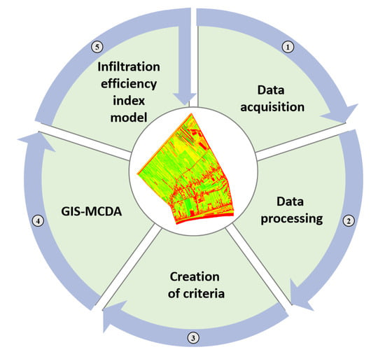
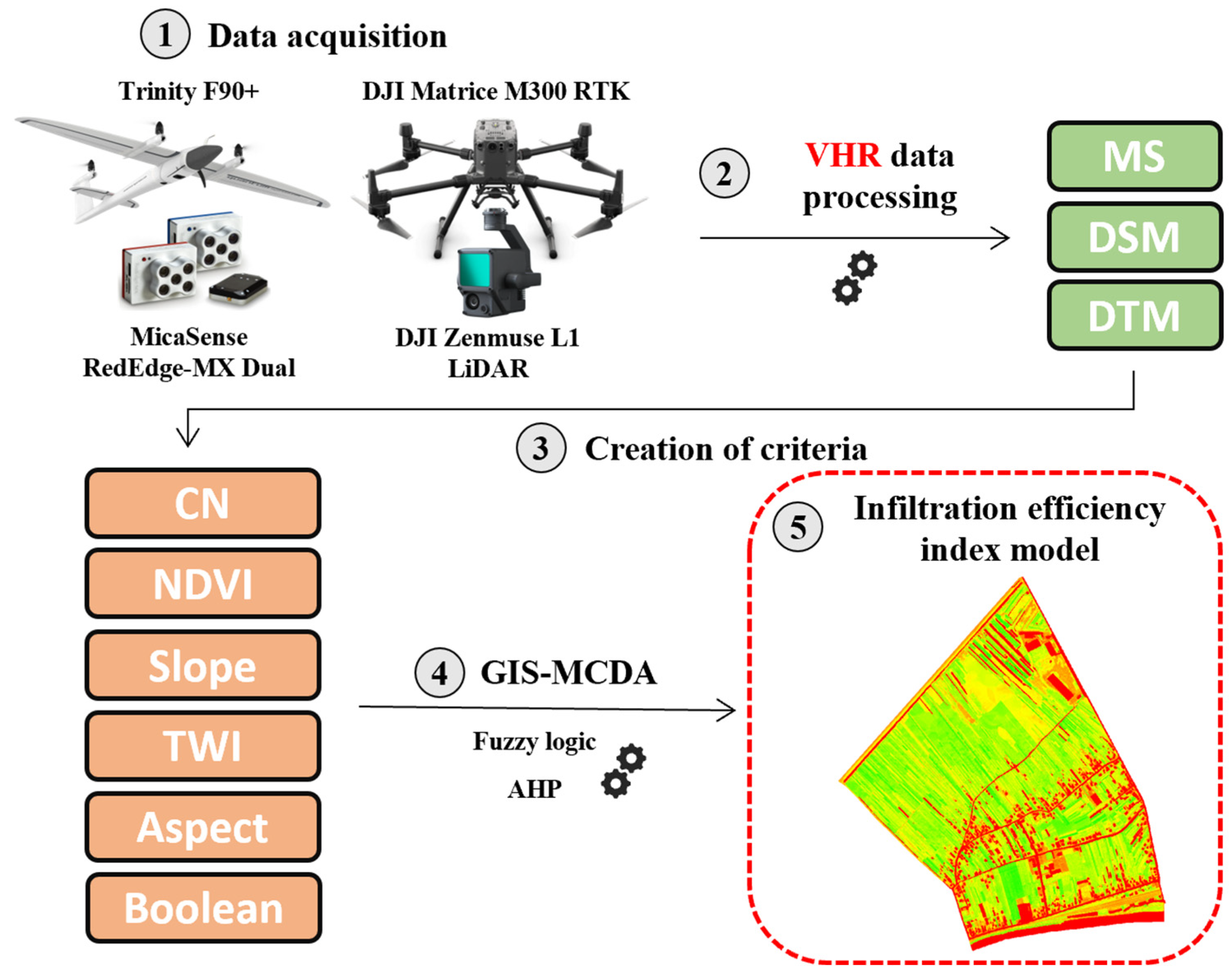
2.2. The Research Methodology
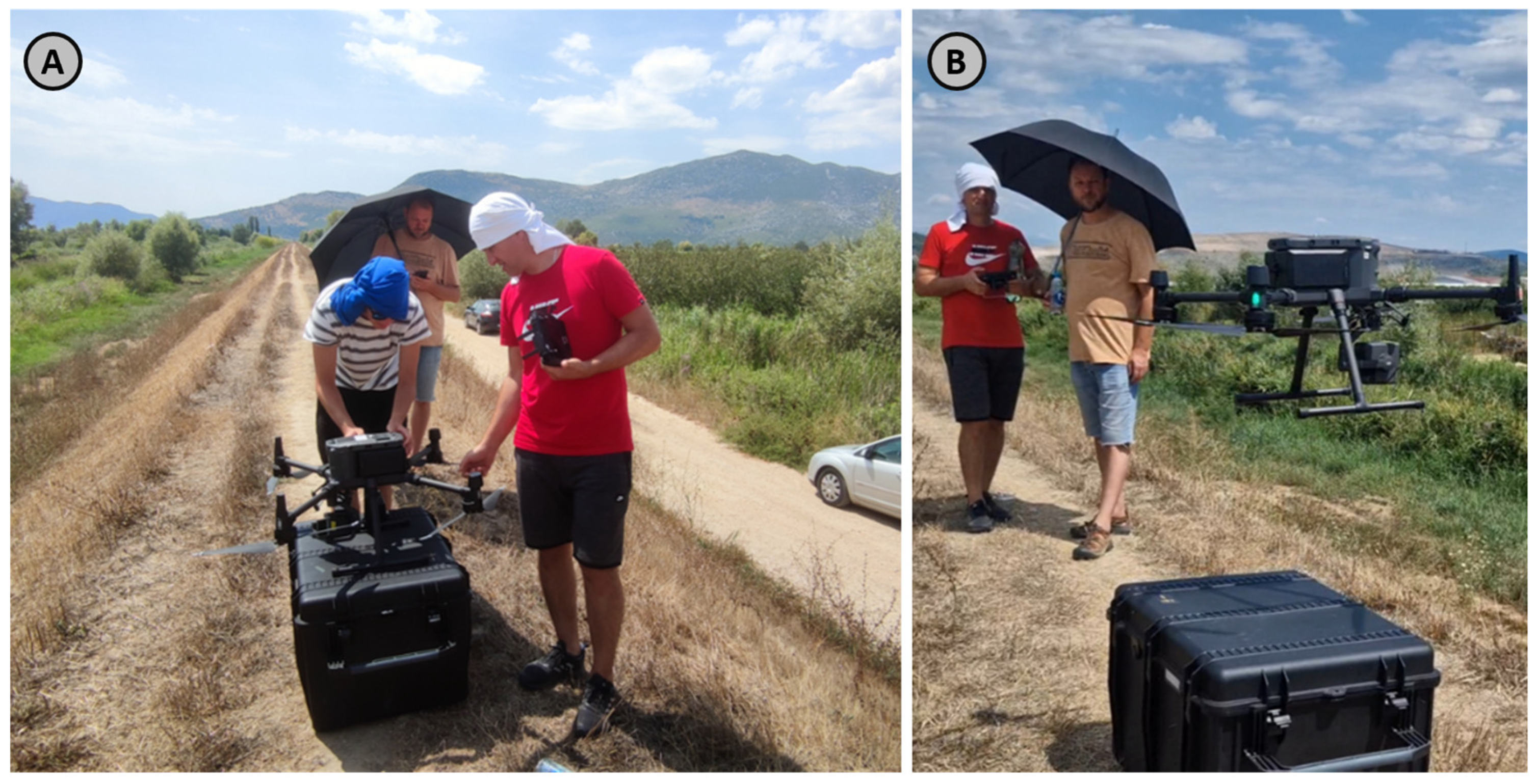
2.3. Data Acquisition
2.3.1. UAV Multispectral Survey
2.3.2. UAV LiDAR Survey
2.4. Data Processing
2.4.1. UAVMS Data Processing
2.4.2. LiDAR Data Processing
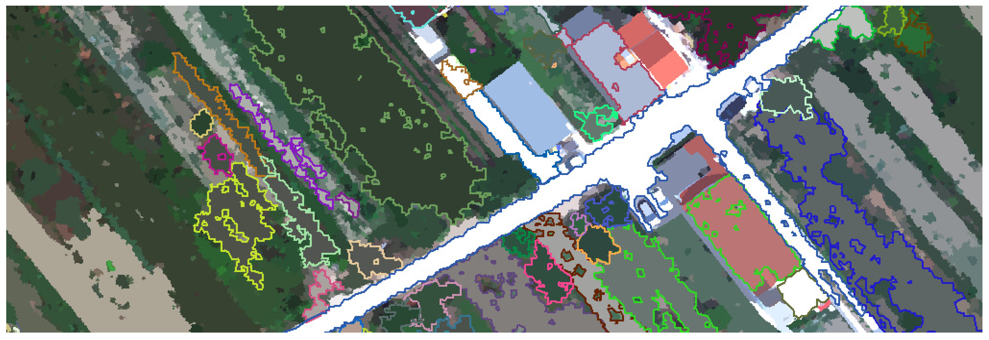
2.5. Creation of Very-High-Resolution Models/Criteria
2.5.1. CN and IS
2.5.2. Normalized Difference Vegetation Index (NDVI)
2.5.3. Slope
2.5.4. Topographic Wetness Index (TWI)
2.5.5. Slope Orientation (Aspect)
2.6. GIS-MCDA
3. Results and Discussion
3.1. Acquired VHR Data
3.2. Derived VHR Models
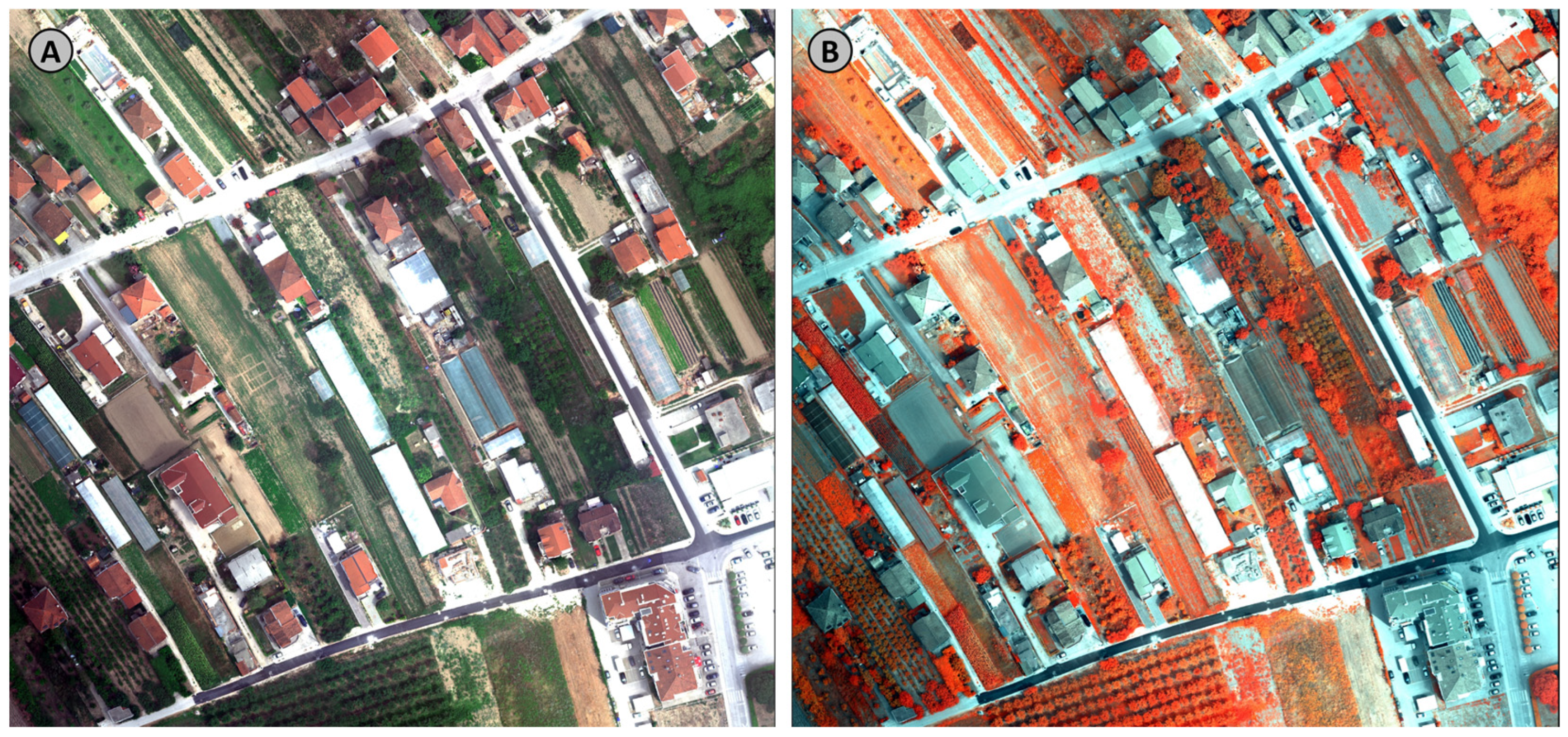
3.2.1. UAVMS
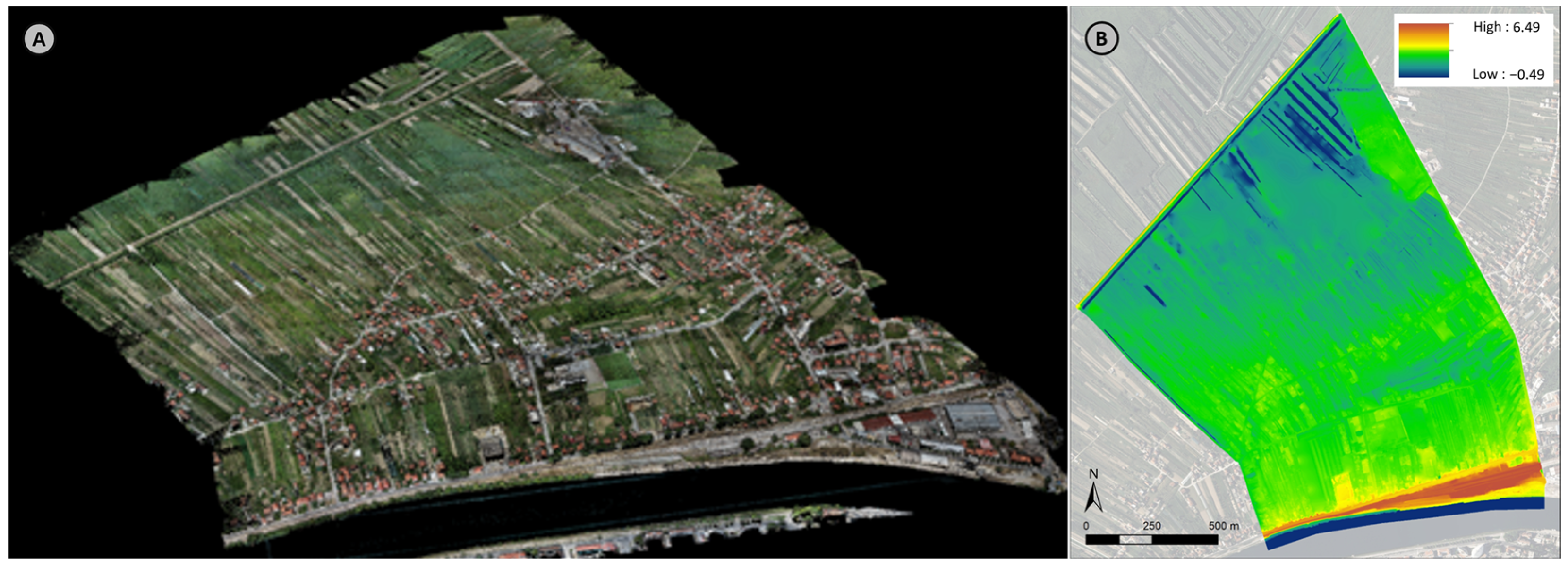
3.2.2. DSM and DTM
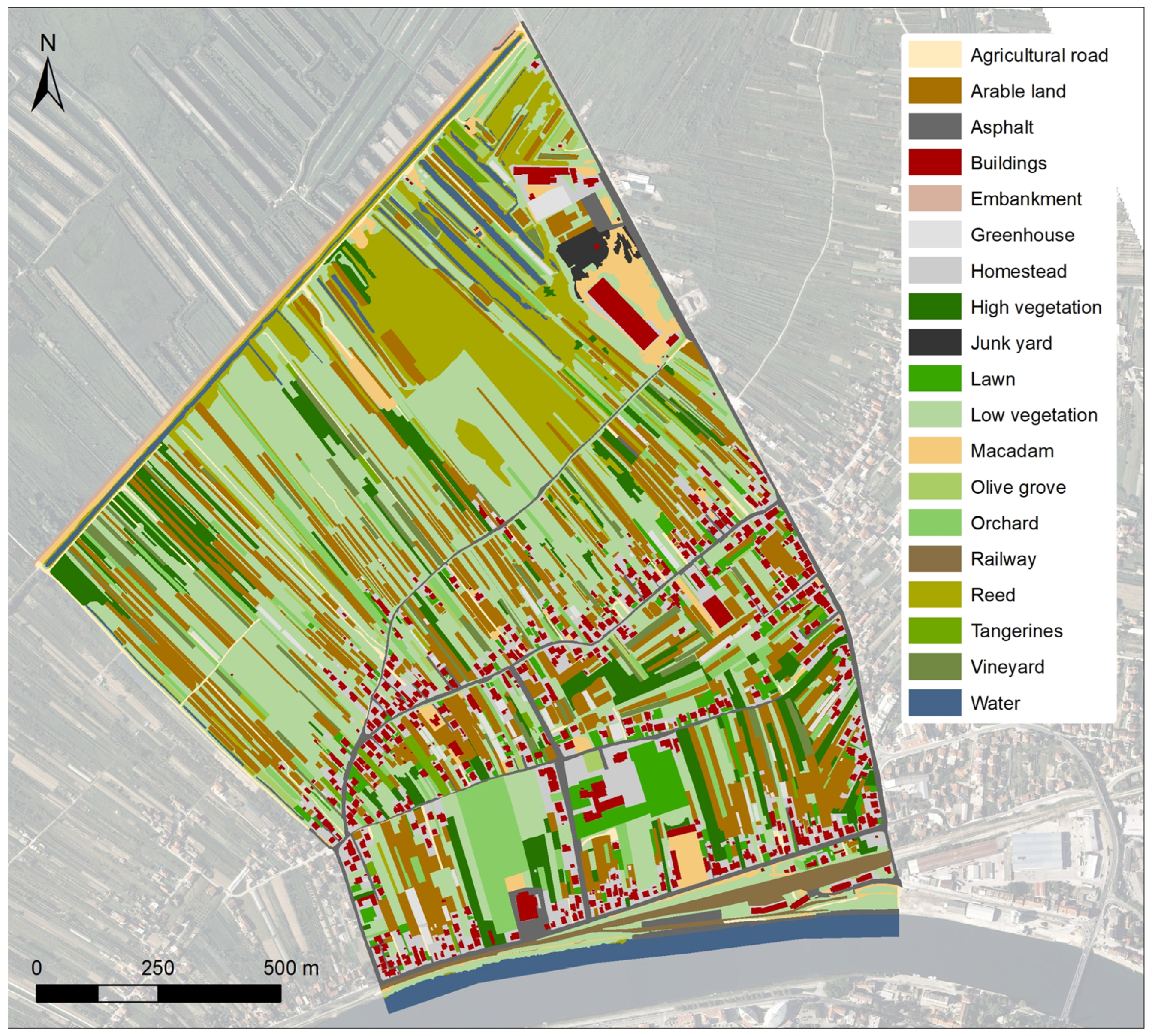
3.2.3. LULC, CN, and IS
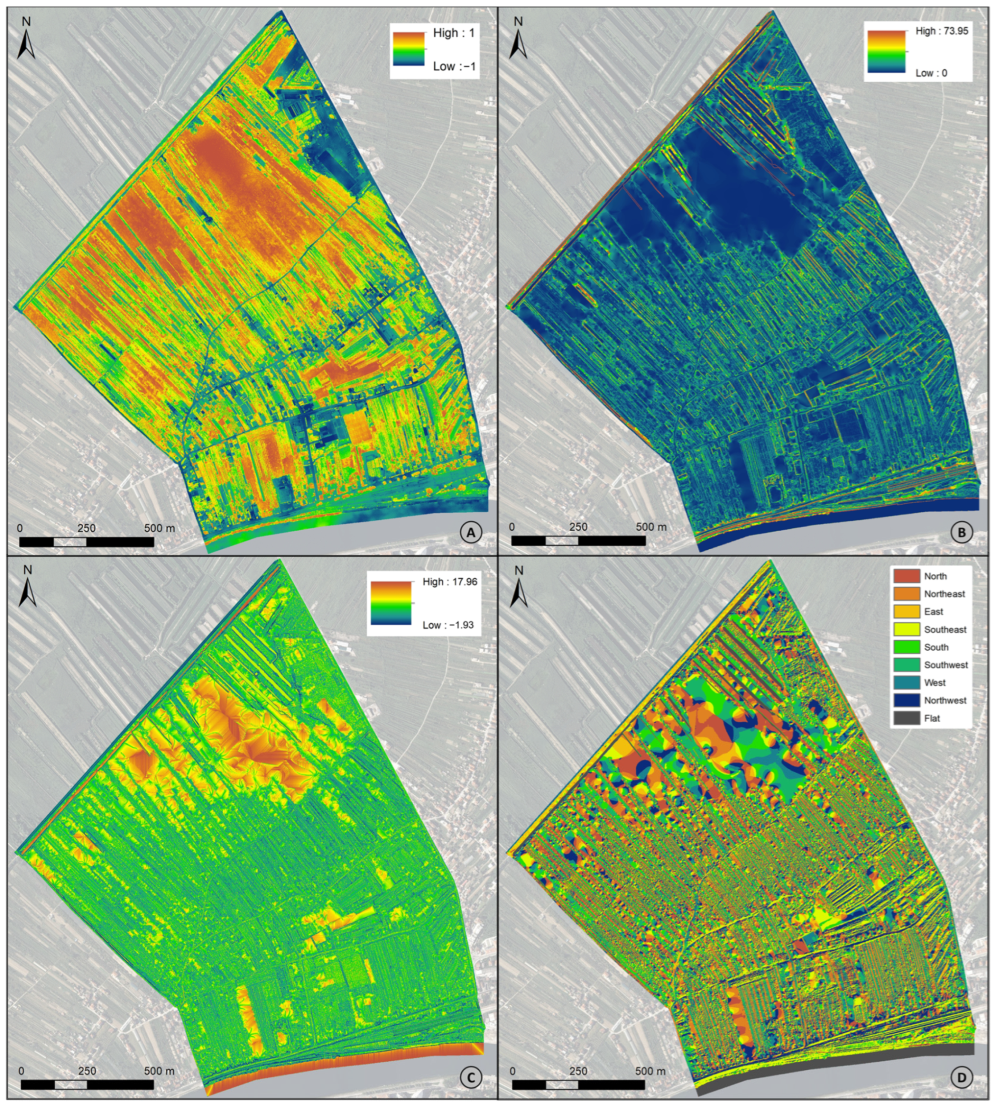
3.2.4. The NDVI
3.2.5. Slope
3.2.6. The TWI
3.2.7. Aspect Model
3.3. GIS-MCDA
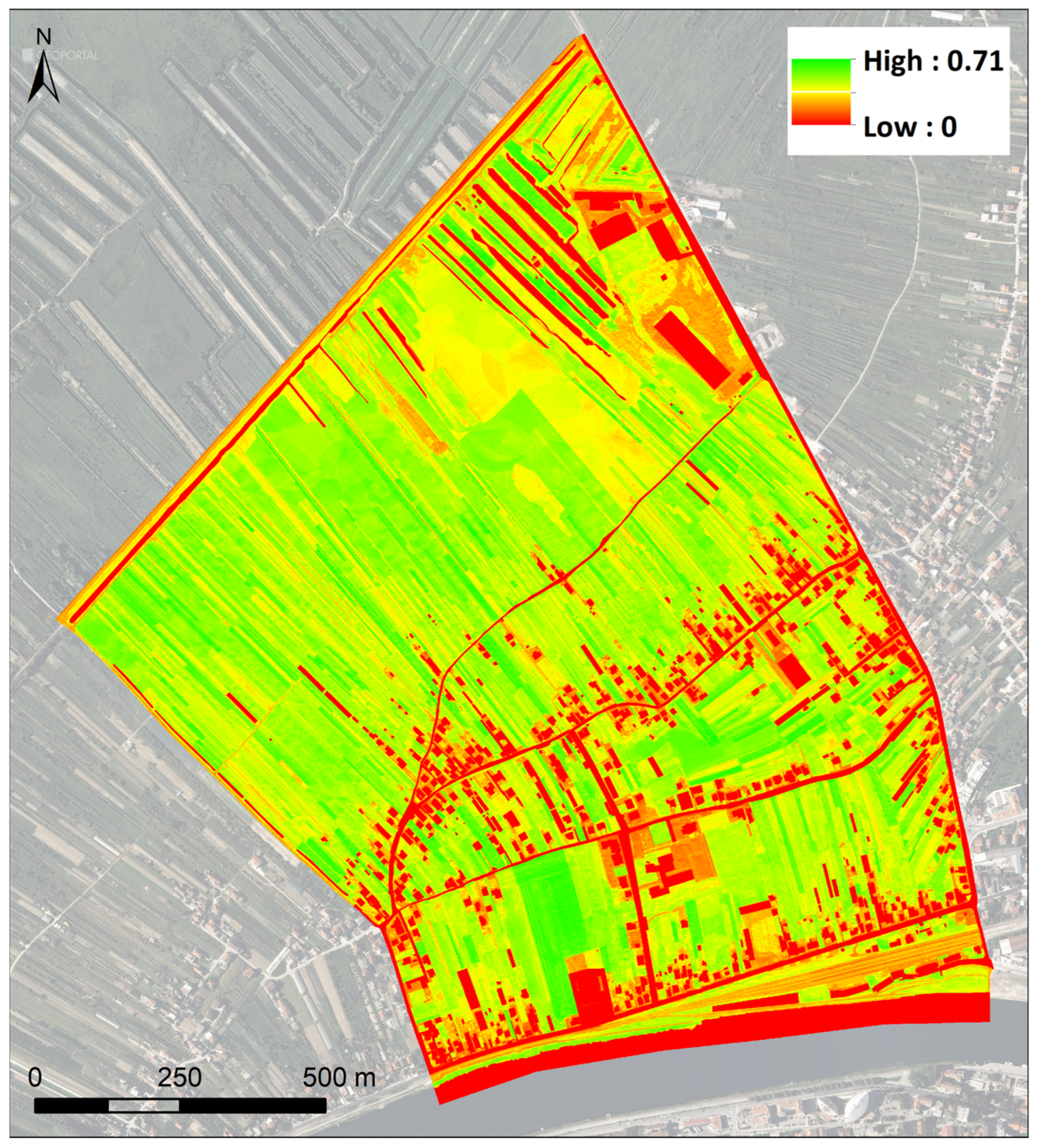
Infiltration Efficiency Index Model
4. Conclusions
Author Contributions
Funding
Data Availability Statement
Conflicts of Interest
References
- Arnold, C.L.; Gibbons, C.J. Impervious Surface Coverage: The Emergence of a Key Environmental Indicator. J. Am. Plan. Assoc. 1996, 62, 243–258. [Google Scholar] [CrossRef]
- Weng, Q. Remote Sensing of Impervious Surfaces in the Urban Areas: Requirements, Methods, and Trends. Remote Sens. Environ. 2012, 117, 34–49. [Google Scholar] [CrossRef]
- Hallegatte, S.; Green, C.; Nicholls, R.J.; Corfee-Morlot, J. Future Flood Losses in Major Coastal Cities. Nat. Clim. Chang. 2013, 3, 802–806. [Google Scholar] [CrossRef]
- Duan, C.; Zhang, J.; Chen, Y.; Lang, Q.; Zhang, Y.; Wu, C.; Zhang, Z. Comprehensive Risk Assessment of Urban Waterlogging Disaster Based on MCDA-GIS Integration: The Case Study of Changchun, China. Remote Sens. 2022, 14, 3101. [Google Scholar] [CrossRef]
- Yu, H.; Zhao, Y.; Fu, Y.; Li, L. Spatiotemporal Variance Assessment of Urban Rainstorm Waterlogging Affected by Impervious Surface Expansion: A Case Study of Guangzhou, China. Sustainability 2018, 10, 3761. [Google Scholar] [CrossRef]
- Sohn, W.; Kim, J.-H.; Li, M.-H.; Brown, R.D.; Jaber, F.H. How Does Increasing Impervious Surfaces Affect Urban Flooding in Response to Climate Variability? Ecol. Indic. 2020, 118, 106774. [Google Scholar] [CrossRef]
- Doerr, S.H.; Shakesby, R.A.; Walsh, R.P.D. Soil Water Repellency: Its Causes, Characteristics and Hydro-Geomorphological Significance. Earth-Sci. Rev. 2000, 51, 33–65. [Google Scholar] [CrossRef]
- Brun, S.E.; Band, L.E. Simulating Runoff Behavior in an Urbanizing Watershed. Comput. Environ. Urban Syst. 2000, 24, 5–22. [Google Scholar] [CrossRef]
- Fu, Y.; Liu, K.; Shen, Z.; Deng, J.; Gan, M.; Liu, X.; Lu, D.; Wang, K. Mapping Impervious Surfaces in Town–Rural Transition Belts Using China’s GF-2 Imagery and Object-Based Deep CNNs. Remote Sens. 2019, 11, 280. [Google Scholar] [CrossRef]
- Ellis, J.B. Sustainable Surface Water Management and Green Infrastructure in UK Urban Catchment Planning. J. Environ. Plan. Manag. 2013, 56, 24–41. [Google Scholar] [CrossRef]
- Wu, C. Quantifying High-resolution Impervious Surfaces Using Spectral Mixture Analysis. Int. J. Remote Sens. 2009, 30, 2915–2932. [Google Scholar] [CrossRef]
- Shuster, W.D.; Bonta, J.; Thurston, H.; Warnemuende, E.; Smith, D.R. Impacts of Impervious Surface on Watershed Hydrology: A Review. Urban Water J. 2005, 2, 263–275. [Google Scholar] [CrossRef]
- Dietz, M.E.; Clausen, J.C. Stormwater Runoff and Export Changes with Development in a Traditional and Low Impact Subdivision. J. Environ. Manag. 2008, 87, 560–566. [Google Scholar] [CrossRef]
- Liu, Z.; Wang, Y.; Li, Z.; Peng, J. Impervious Surface Impact on Water Quality in the Process of Rapid Urbanization in Shenzhen, China. Environ. Earth Sci. 2013, 68, 2365–2373. [Google Scholar] [CrossRef]
- Kim, H.; Jeong, H.; Jeon, J.; Bae, S. The Impact of Impervious Surface on Water Quality and Its Threshold in Korea. Water 2016, 8, 111. [Google Scholar] [CrossRef]
- Feng, B.; Zhang, Y.; Bourke, R. Urbanization Impacts on Flood Risks Based on Urban Growth Data and Coupled Flood Models. Nat. Hazards 2021, 106, 613–627. [Google Scholar] [CrossRef]
- Deng, C.; Wu, C. BCI: A Biophysical Composition Index for Remote Sensing of Urban Environments. Remote Sens. Environ. 2012, 127, 247–259. [Google Scholar] [CrossRef]
- Liu, C.; Shao, Z.; Chen, M.; Luo, H. MNDISI: A Multi-Source Composition Index for Impervious Surface Area Estimation at the Individual City Scale. Remote Sens. Lett. 2013, 4, 803–812. [Google Scholar] [CrossRef]
- Sun, G.; Chen, X.; Jia, X.; Yao, Y.; Wang, Z. Combinational Build-Up Index (CBI) for Effective Impervious Surface Mapping in Urban Areas. IEEE J. Sel. Top. Appl. Earth Obs. Remote Sens. 2016, 9, 2081–2092. [Google Scholar] [CrossRef]
- Wu, C. Normalized Spectral Mixture Analysis for Monitoring Urban Composition Using ETM+ Imagery. Remote Sens. Environ. 2004, 93, 480–492. [Google Scholar] [CrossRef]
- Herold, M.; Roberts, D.A.; Gardner, M.E.; Dennison, P.E. Spectrometry for Urban Area Remote Sensing—Development and Analysis of a Spectral Library from 350 to 2400 Nm. Remote Sens. Environ. 2004, 91, 304–319. [Google Scholar] [CrossRef]
- Yang, J.; He, Y. Automated Mapping of Impervious Surfaces in Urban and Suburban Areas: Linear Spectral Unmixing of High Spatial Resolution Imagery. Int. J. Appl. Earth Obs. Geoinf. 2017, 54, 53–64. [Google Scholar] [CrossRef]
- Okujeni, A.; van der Linden, S.; Tits, L.; Somers, B.; Hostert, P. Support Vector Regression and Synthetically Mixed Training Data for Quantifying Urban Land Cover. Remote Sens. Environ. 2013, 137, 184–197. [Google Scholar] [CrossRef]
- Ou, J.; Liu, X.; Liu, P.; Liu, X. Evaluation of Luojia 1-01 Nighttime Light Imagery for Impervious Surface Detection: A Comparison with NPP-VIIRS Nighttime Light Data. Int. J. Appl. Earth Obs. Geoinf. 2019, 81, 1–12. [Google Scholar] [CrossRef]
- Sun, Z. Estimating Urban Impervious Surfaces from Landsat-5 TM Imagery Using Multilayer Perceptron Neural Network and Support Vector Machine. J. Appl. Remote Sens. 2011, 5, 053501. [Google Scholar] [CrossRef]
- Okujeni, A.; Canters, F.; Cooper, S.D.; Degerickx, J.; Heiden, U.; Hostert, P.; Priem, F.; Roberts, D.A.; Somers, B.; van der Linden, S. Generalizing Machine Learning Regression Models Using Multi-Site Spectral Libraries for Mapping Vegetation-Impervious-Soil Fractions across Multiple Cities. Remote Sens. Environ. 2018, 216, 482–496. [Google Scholar] [CrossRef]
- Zhang, L.; Zhang, M.; Yao, Y. Mapping Seasonal Impervious Surface Dynamics in Wuhan Urban Agglomeration, China from 2000 to 2016. Int. J. Appl. Earth Obs. Geoinf. 2018, 70, 51–61. [Google Scholar] [CrossRef]
- The European Environment. State and Outlook 2020: Knowledge for Transition to a Sustainable Europe—European Environment Agency. Available online: https://www.eea.europa.eu/soer/2020 (accessed on 5 June 2023).
- Vysna, V.; Maes, J.; Petersen, J.-E.; La Notte, A.; Vallecillo, S.; Aizpurua, N.; Ivits, E.; Teller, A. Accounting for Ecosystems and Their Services in the European Union (INCA): Final Report from Phase II of the INCA Project Aiming to Develop a Pilot for an Integrated System of Ecosystem Accounts for the EU: 2021 Edition; Publications Office of the European Union: Luxembourg, 2020; ISBN 978-92-76-17401-1. [Google Scholar]
- Strand, G.-H. Accuracy of the Copernicus High-Resolution Layer Imperviousness Density (HRL IMD) Assessed by Point Sampling within Pixels. Remote Sens. 2022, 14, 3589. [Google Scholar] [CrossRef]
- Krvavica, N.; Šiljeg, A.; Horvat, B.; Panđa, L. Pluvial Flash Flood Hazard and Risk Mapping in Croatia: Case Study in the Gospić Catchment. Sustainability 2023, 15, 1197. [Google Scholar] [CrossRef]
- Imperviousness—Copernicus Land Monitoring Service. Available online: https://land.copernicus.eu/pan-european/high-resolution-layers/imperviousness (accessed on 30 April 2023).
- Mangala, O.S.; Toppo, P.; Ghoshal, S. Study of Infiltration Capacity of Different Soils. Int. J. Trend Res. Dev. 2016, 3, 388–390. [Google Scholar]
- Horton, R.E. An Approach Toward a Physical Interpretation of Infiltration-Capacity. Soil Sci. Soc. Am. J. 1941, 5, 399–417. [Google Scholar] [CrossRef]
- Yimer, F.; Messing, I.; Ledin, S.; Abdelkadir, A. Effects of Different Land Use Types on Infiltration Capacity in a Catchment in the Highlands of Ethiopia. Soil Use Manag. 2008, 24, 344–349. [Google Scholar] [CrossRef]
- Sun, D.; Yang, H.; Guan, D.; Yang, M.; Wu, J.; Yuan, F.; Jin, C.; Wang, A.; Zhang, Y. The Effects of Land Use Change on Soil Infiltration Capacity in China: A Meta-Analysis. Sci. Total Environ. 2018, 626, 1394–1401. [Google Scholar] [CrossRef]
- USDA. Chapter 9: Hydrological Soil-Cover Complexes. In USDA National Engineering Handbook; USDA: Washington, DC, USA, 2004. Available online: https://directives.sc.egov.usda.gov/viewerfs.aspx?hid=21422 (accessed on 9 May 2023).
- Hong, Y.; Adler, R.F. Estimation of Global SCS Curve Numbers Using Satellite Remote Sensing and Geospatial Data. Int. J. Remote Sens. 2008, 29, 471–477. [Google Scholar] [CrossRef]
- Hoeft, C.C. Incorporating Updated Runoff Curve Number Technology into NRCS Directives. In Watershed Management 2020: A Clear Vision of Watershed Management; ASCE: Reston, VA, USA, 2020; pp. 78–87. [Google Scholar] [CrossRef]
- Akan, A.O. Horton Infiltration Equation Revisited. J. Irrig. Drain. Eng. 1992, 118, 828–830. [Google Scholar] [CrossRef]
- Rawls, W.J.; Brakensiek, D.L.; Miller, N. Green-ampt Infiltration Parameters from Soils Data. J. Hydraul. Eng. 1983, 109, 62–70. [Google Scholar] [CrossRef]
- Dahak, A.; Boutaghane, H.; Merabtene, T. Parameter Estimation and Assessment of Infiltration Models for Madjez Ressoul Catchment, Algeria. Water 2022, 14, 1185. [Google Scholar] [CrossRef]
- Miyata, S.; Gomi, T.; Sidle, R.C.; Onda, Y.; Yamamoto, K.; Nonoda, T.; Hiraoka, M.; Kosugi, K. Evaluation of Spatial Patterns of Infiltration Capacity on Storm Runoff in a Forested Watershed: Utilizing of LiDAR Data in a Distributed Runoff Model. In Proceedings of the American Geophysical Union Fall Meeting, San Francisco, CA, USA, 15–19 December 2008. [Google Scholar]
- Langhans, C.; Govers, G.; Diels, J.; Leys, A.; Clymans, W.; den Putte, A.V.; Valckx, J. Experimental Rainfall–Runoff Data: Reconsidering the Concept of Infiltration Capacity. J. Hydrol. 2011, 399, 255–262. [Google Scholar] [CrossRef]
- Nuottimäki, K.; Jarva, J. A Qualitative Approach for Identifying Areas Prone to Urban Floods with the Support of LiDAR. GFF 2015, 137, 373–382. [Google Scholar] [CrossRef]
- McGuire, L.A.; Rengers, F.K.; Kean, J.W.; Staley, D.M.; Mirus, B.B. Incorporating Spatially Heterogeneous Infiltration Capacity into Hydrologic Models with Applications for Simulating Post-Wildfire Debris Flow Initiation. Hydrol. Process. 2018, 32, 1173–1187. [Google Scholar] [CrossRef]
- Miyata, S.; Gomi, T.; Sidle, R.C.; Hiraoka, M.; Onda, Y.; Yamamoto, K.; Nonoda, T. Assessing Spatially Distributed Infiltration Capacity to Evaluate Storm Runoff in Forested Catchments: Implications for Hydrological Connectivity. Sci. Total Environ. 2019, 669, 148–159. [Google Scholar] [CrossRef]
- Roca, D.; Armesto, J.; Lagüela, S.; Díaz-Vilariño, L. Lidar-Equipped Uav for Building Information Modelling. Int. Arch. Photogramm. Remote Sens. Spat. Inf. Sci. 2014, XL-5, 523–527. [Google Scholar] [CrossRef]
- Luo, H.; Wang, L.; Wu, C.; Zhang, L. An Improved Method for Impervious Surface Mapping Incorporating LiDAR Data and High-Resolution Imagery at Different Acquisition Times. Remote Sens. 2018, 10, 1349. [Google Scholar] [CrossRef]
- Baby, S.N.; Arrowsmith, C.; Liu, G.-J.; Mitchell, D.; Al-Ansari, N.; Abbas, N. Finding Areas at Risk from Floods in a Downpour Using the Lidar-Based Elevation Model. J. Civ. Eng. Archit. 2021, 15, 1–16. Available online: https://www.researchgate.net/publication/349098888_Finding_Areas_at_Risk_from_Floods_in_a_Downpour_Using_the_Lidar-Based_Elevation_Model (accessed on 30 May 2023).
- Chapa, F.; Hariharan, S.; Hack, J. A New Approach to High-Resolution Urban Land Use Classification Using Open Access Software and True Color Satellite Images. Sustainability 2019, 11, 5266. [Google Scholar] [CrossRef]
- Qu, L.; Chen, Z.; Li, M.; Zhi, J.; Wang, H. Accuracy Improvements to Pixel-Based and Object-Based Lulc Classification with Auxiliary Datasets from Google Earth Engine. Remote Sens. 2021, 13, 453. [Google Scholar] [CrossRef]
- Khosravi, K.; Pham, B.T.; Chapi, K.; Shirzadi, A.; Shahabi, H.; Revhaug, I.; Prakash, I.; Tien Bui, D. A Comparative Assessment of Decision Trees Algorithms for Flash Flood Susceptibility Modeling at Haraz Watershed, Northern Iran. Sci. Total Environ. 2018, 627, 744–755. [Google Scholar] [CrossRef]
- Khosravi, K.; Shahabi, H.; Pham, B.T.; Adamowski, J.; Shirzadi, A.; Pradhan, B.; Dou, J.; Ly, H.-B.; Gróf, G.; Ho, H.L.; et al. A Comparative Assessment of Flood Susceptibility Modeling Using Multi-Criteria Decision-Making Analysis and Machine Learning Methods. J. Hydrol. 2019, 573, 311–323. [Google Scholar] [CrossRef]
- Wang, Y.; Hong, H.; Chen, W.; Li, S.; Pamučar, D.; Gigović, L.; Drobnjak, S.; Tien Bui, D.; Duan, H. A Hybrid GIS Multi-Criteria Decision-Making Method for Flood Susceptibility Mapping at Shangyou, China. Remote Sens. 2019, 11, 62. [Google Scholar] [CrossRef]
- Gudiyangada Nachappa, T.; Tavakkoli Piralilou, S.; Gholamnia, K.; Ghorbanzadeh, O.; Rahmati, O.; Blaschke, T. Flood Susceptibility Mapping with Machine Learning, Multi-Criteria Decision Analysis and Ensemble Using Dempster Shafer Theory. J. Hydrol. 2020, 590, 125275. [Google Scholar] [CrossRef]
- Birch, G.F.; Fazeli, M.S.; Matthai, C. Efficiency of an infiltration basin in removing contaminants from urban stormwater. Env. Monit Assess 2005, 101, 23–38. [Google Scholar] [CrossRef]
- Widomski, M.K.; Sobczuk, H.; Olszta, W. Sand-Filled Drainage Ditches for Erosion Control: Effects on Infiltration Efficiency. Soil Sci. Soc. Am. J. 2010, 74, 213–220. [Google Scholar] [CrossRef]
- De Carlo, L.; Caputo, M.C.; Masciale, R.; Vurro, M.; Portoghese, I. Monitoring the Drainage Efficiency of Infiltration Trenches in Fractured and Karstified Limestone via Time-Lapse Hydrogeophysical Approach. Water 2020, 12, 2009. [Google Scholar] [CrossRef]
- Archer, N.A.L.; Bell, R.A.; Butcher, A.S.; Bricker, S.H. Infiltration Efficiency and Subsurface Water Processes of a Sustainable Drainage System and Consequences to Flood Management. J. Flood Risk Manag. 2020, 13, e12629. [Google Scholar] [CrossRef]
- Državni Zavod Za Statistiku. Popis ‘21. Available online: https://popis2021.hr/ (accessed on 30 March 2022).
- Docs&Tools—STREAM—Italia-Croatia. Available online: https://programming14-20.italy-croatia.eu/web/stream/docs-and-tools (accessed on 23 October 2023).
- Galić, J. Regionalizacija Donjoneretvanske Delte. Naše More Znan. Časopis Za More I Pomor. 2011, 58, 39–46. [Google Scholar]
- Šiljković, Ž.; Glamuzina, M. Mogućnost Uvođenja Eko–Poljoprivrede u Deltu Neretve. Soc. Ekol. Časopis Za Ekološku Misao I Sociol. Istraživanja Okoline 1999, 8, 183–191. [Google Scholar]
- DHMZ Croatian Meteorological and Hydrological Service. Climate Atlas of Croatia 1961–1990, 1971–2000; DHMZ: Zagreb, Croatia, 2008; Available online: https://klima.hr/razno/publikacije/klimatski_atlas_hrvatske.pdf (accessed on 30 May 2023).
- Discover Trinity F90+. The Unbeatable Mapping Drone. Available online: https://quantum-systems.com/trinity-f90/ (accessed on 30 May 2023).
- Comparison of MicaSense Cameras. Available online: https://support.micasense.com/hc/en-us/articles/1500007828482-Comparison-of-MicaSense-Cameras (accessed on 30 May 2023).
- Maté-González, M.Á.; Di Pietra, V.; Piras, M. Evaluation of Different LiDAR Technologies for the Documentation of Forgotten Cultural Heritage under Forest Environments. Sensors 2022, 22, 6314. [Google Scholar] [CrossRef]
- Alphonse, A.B.; Wawrzyniak, T.; Osuch, M.; Hanselmann, N. Applying UAV-Based Remote Sensing Observation Products in High Arctic Catchments in SW Spitsbergen. Remote Sens. 2023, 15, 934. [Google Scholar] [CrossRef]
- Mitka, B.; Klapa, P.; Pióro, P. Acquisition and Processing Data from UAVs in the Process of Generating 3D Models for Solar Potential Analysis. Remote Sens. 2023, 15, 1498. [Google Scholar] [CrossRef]
- Zenmuse L1. UAV Load Gimbal Camera—DJI Enterprise. Available online: https://enterprise.dji.com/photo (accessed on 16 May 2023).
- Dearden, R.A.; Marchant, A.; Royse, K. Development of a Suitability Map for Infiltration Sustainable Drainage Systems (SuDS). Env. Earth Sci. 2013, 70, 2587–2602. [Google Scholar] [CrossRef]
- Blaschke, T. Object Based Image Analysis for Remote Sensing. ISPRS J. Photogramm. Remote Sens. 2010, 65, 2–16. [Google Scholar] [CrossRef]
- MacFaden, S.W.; O’Neil-Dunne, J.P.M.; Royar, A.R.; Lu, J.W.T.; Rundle, A.G. High-Resolution Tree Canopy Mapping for New York City Using LIDAR and Object-Based Image Analysis. J. Appl. Remote Sens. 2012, 6, 063567. [Google Scholar] [CrossRef]
- Hay, G.J.; Castilla, G. Geographic Object-Based Image Analysis (GEOBIA): A New Name for a New Discipline. In Object-Based Image Analysis: Spatial Concepts for Knowledge-Driven Remote Sensing Applications; Blaschke, T., Lang, S., Hay, G.J., Eds.; Lecture Notes in Geoinformation and Cartography; Springer: Berlin/Heidelberg, Germany, 2008; pp. 75–89. ISBN 978-3-540-77058-9. [Google Scholar]
- Lang, S. Object-Based Image Analysis for Remote Sensing Applications: Modeling Reality—Dealing with Complexity. In Object-Based Image Analysis; Springer: Berlin/Heidelberg, Germany, 2008; Available online: https://link.springer.com/book/10.1007/978-3-540-77058-9 (accessed on 12 April 2023).
- Comaniciu, D.; Meer, P. Mean Shift: A Robust Approach toward Feature Space Analysis. IEEE Trans. Pattern Anal. Mach. Intell. 2002, 24, 603–619. [Google Scholar] [CrossRef]
- Millard, K.; Richardson, M. On the Importance of Training Data Sample Selection in Random Forest Image Classification: A Case Study in Peatland Ecosystem Mapping. Remote Sens. 2015, 7, 8489–8515. [Google Scholar] [CrossRef]
- Ye, S.; Pontius, R.G.; Rakshit, R. A Review of Accuracy Assessment for Object-Based Image Analysis: From per-Pixel to per-Polygon Approaches. ISPRS J. Photogramm. Remote Sens. 2018, 141, 137–147. [Google Scholar] [CrossRef]
- Dixon, B.; Candade, N. Multispectral Landuse Classification Using Neural Networks and Support Vector Machines: One or the Other, or Both? Int. J. Remote Sens. 2008, 29, 1185–1206. [Google Scholar] [CrossRef]
- Gibril, M.B.A.; Bakar, S.A.; Yao, K.; Idrees, M.O.; Pradhan, B. Fusion of RADARSAT-2 and Multispectral Optical Remote Sensing Data for LULC Extraction in a Tropical Agricultural Area. Geocarto Int. 2017, 32, 735–748. [Google Scholar] [CrossRef]
- Fragou, S.; Kalogeropoulos, K.; Stathopoulos, N.; Louka, P.; Srivastava, P.K.; Karpouzas, S.; Kalivas, D.P.; Petropoulos, G.P. Quantifying Land Cover Changes in a Mediterranean Environment Using Landsat TM and Support Vector Machines. Forests 2020, 11, 750. [Google Scholar] [CrossRef]
- Oo, T.K.; Arunrat, N.; Sereenonchai, S.; Ussawarujikulchai, A.; Chareonwong, U.; Nutmagul, W. Comparing Four Machine Learning Algorithms for Land Cover Classification in Gold Mining: A Case Study of Kyaukpahto Gold Mine, Northern Myanmar. Sustainability 2022, 14, 10754. [Google Scholar] [CrossRef]
- Train Support Vector Machine Classifier (Spatial Analyst)—ArcMap | Documentation. Available online: https://desktop.arcgis.com/en/arcmap/latest/tools/spatial-analyst-toolbox/train-support-vector-machine-classifier.htm (accessed on 17 August 2023).
- Congalton, R.G. A Review of Assessing the Accuracy of Classifications of Remotely Sensed Data. Remote Sens. Environ. 1991, 37, 35–46. [Google Scholar] [CrossRef]
- Liu, C.; Frazier, P.; Kumar, L. Comparative Assessment of the Measures of Thematic Classification Accuracy. Remote Sens. Environ. 2007, 107, 606–616. [Google Scholar] [CrossRef]
- Thompson, W.D.; Walter, S.D. A Reappraisal of the Kappa Coefficient. J. Clin. Epidemiol. 1988, 41, 949–958. [Google Scholar] [CrossRef]
- Rigby, A.S. Statistical Methods in Epidemiology. v. Towards an Understanding of the Kappa Coefficient. Disabil. Rehabil. 2000, 22, 339–344. [Google Scholar] [CrossRef] [PubMed]
- Koukoulas, S.; Blackburn, G.A. Mapping Individual Tree Location, Height and Species in Broadleaved Deciduous Forest Using Airborne LIDAR and Multi-spectral Remotely Sensed Data. Int. J. Remote Sens. 2005, 26, 431–455. [Google Scholar] [CrossRef]
- Šiljeg, A.; Panđa, L.; Domazetović, F.; Marić, I.; Gašparović, M.; Borisov, M.; Milošević, R. Comparative Assessment of Pixel and Object-Based Approaches for Mapping of Olive Tree Crowns Based on UAV Multispectral Imagery. Remote Sens. 2022, 14, 757. [Google Scholar] [CrossRef]
- Kou, X.; Han, D.; Cao, Y.; Shang, H.; Li, H.; Zhang, X.; Yang, M. Acid Mine Drainage Discrimination Using Very High Resolution Imagery Obtained by Unmanned Aerial Vehicle in a Stone Coal Mining Area. Water 2023, 15, 1613. [Google Scholar] [CrossRef]
- Park, G.; Park, K.; Song, B.; Lee, H. Analyzing Impact of Types of UAV-Derived Images on the Object-Based Classification of Land Cover in an Urban Area. Drones 2022, 6, 71. [Google Scholar] [CrossRef]
- Jozdani, S.E.; Johnson, B.A.; Chen, D. Comparing Deep Neural Networks, Ensemble Classifiers, and Support Vector Machine Algorithms for Object-Based Urban Land Use/Land Cover Classification. Remote Sens. 2019, 11, 1713. [Google Scholar] [CrossRef]
- Lu, D.; Weng, Q. A Survey of Image Classification Methods and Techniques for Improving Classification Performance. Int. J. Remote Sens. 2007, 28, 823–870. [Google Scholar] [CrossRef]
- Abdullah, A.Y.M.; Masrur, A.; Adnan, M.S.G.; Baky, M.A.A.; Hassan, Q.K.; Dewan, A. Spatio-Temporal Patterns of Land Use/Land Cover Change in the Heterogeneous Coastal Region of Bangladesh between 1990 and 2017. Remote Sens. 2019, 11, 790. [Google Scholar] [CrossRef]
- Wardlow, B.D.; Egbert, S.L. Large-Area Crop Mapping Using Time-Series MODIS 250 m NDVI Data: An Assessment for the US Central Great Plains. Remote Sens. Environ. 2008, 112, 1096–1116. [Google Scholar] [CrossRef]
- Malinverni, E.S.; Tassetti, A.N.; Mancini, A.; Zingaretti, P.; Frontoni, E.; Bernardini, A. Hybrid Object-Based Approach for Land Use/Land Cover Mapping Using High Spatial Resolution Imagery. Int. J. Geogr. Inf. Sci. 2011, 25, 1025–1043. [Google Scholar] [CrossRef]
- Rajendran, G.B.; Kumarasamy, U.M.; Zarro, C.; Divakarachari, P.B.; Ullo, S.L. Land-Use and Land-Cover Classification Using a Human Group-Based Particle Swarm Optimization Algorithm with an LSTM Classifier on Hybrid Pre-Processing Remote-Sensing Images. Remote Sens. 2020, 12, 4135. [Google Scholar] [CrossRef]
- Radočaj, D.; Jurišić, M.; Gašparović, M. The Role of Remote Sensing Data and Methods in a Modern Approach to Fertilization in Precision Agriculture. Remote Sens. 2022, 14, 778. [Google Scholar] [CrossRef]
- Vidaček, Ž.; Bogunović, M.; Husnjak, S.; Sraka, M.; Bensa, A. Hydropedological Map of the Republic of Croatia. Agric. Conspec. Sci. 2008, 73, 67–74. [Google Scholar]
- Gitelson, A.A.; Kaufman, Y.J.; Merzlyak, M.N. Use of a Green Channel in Remote Sensing of Global Vegetation from EOS- MODIS. Remote Sens. Environ. 1996, 58, 289–298. [Google Scholar] [CrossRef]
- Patón, D. Normalized Difference Vegetation Index Determination in Urban Areas by Full-Spectrum Photography. Ecologies 2020, 1, 22–35. [Google Scholar] [CrossRef]
- Huang, S.; Tang, L.; Hupy, J.P.; Wang, Y.; Shao, G. A Commentary Review on the Use of Normalized Difference Vegetation Index (NDVI) in the Era of Popular Remote Sensing. J. For. Res. 2021, 32, 1–6, Erratum in J. For. Res. 2021, 32, 2719. [Google Scholar] [CrossRef]
- Braun, M.; Herold, M. Mapping Imperviousness Using NDVI and Linear Spectral Unmixing of ASTER Data in the Cologne-Bonn Region (Germany). In Proceedings of the Remote Sensing for Environmental Monitoring, GIS Applications, and Geology III, Barcelona, Spain, 8–12 September 2003; SPIE: Paris, France, 2004; Volume 5239, pp. 274–284. [Google Scholar]
- Zhang, Y.; Odeh, I.O.; Han, C. Bi-Temporal Characterization of Land Surface Temperature in Relation to Impervious Surface Area, NDVI and NDBI, Using a Sub-Pixel Image Analysis. Int. J. Appl. Earth Obs. Geoinf. 2009, 11, 256–264. [Google Scholar] [CrossRef]
- Knight, J.; Voth, M. Mapping Impervious Cover Using Multi-Temporal MODIS NDVI Data. IEEE J. Sel. Top. Appl. Earth Obs. Remote Sens. 2010, 4, 303–309. [Google Scholar] [CrossRef]
- Guo, W.; Lu, D.; Wu, Y.; Zhang, J. Mapping Impervious Surface Distribution with Integration of SNNP VIIRS-DNB and MODIS NDVI Data. Remote Sens. 2015, 7, 12459–12477. [Google Scholar] [CrossRef]
- Guo, W.; Lu, D.; Kuang, W. Improving Fractional Impervious Surface Mapping Performance through Combination of DMSP-OLS and MODIS NDVI Data. Remote Sens. 2017, 9, 375. [Google Scholar] [CrossRef]
- Rouse, J.W.; Haas, R.H.; Schell, J.A.; Deering, D.W. Monitoring Vegetation Systems in the Great Plains with ERTS. NASA Spec. Publ. 1974, 351, 309. [Google Scholar]
- Morbidelli, R.; Saltalippi, C.; Flammini, A.; Govindaraju, R.S. Role of Slope on Infiltration: A Review. J. Hydrol. 2018, 557, 878–886. [Google Scholar] [CrossRef]
- Yu, H.; Zhao, Y.; Fu, Y. Optimization of Impervious Surface Space Layout for Prevention of Urban Rainstorm Waterlogging: A Case Study of Guangzhou, China. Int. J. Environ. Res. Public Health 2019, 16, 3613. [Google Scholar] [CrossRef]
- Sytsma, A.; Bell, C.; Eisenstein, W.; Hogue, T.; Kondolf, G.M. A Geospatial Approach for Estimating Hydrological Connectivity of Impervious Surfaces. J. Hydrol. 2020, 591, 125545. [Google Scholar] [CrossRef]
- Meierdiercks, K.L.; Kolozsvary, M.B.; Rhoads, K.P.; Golden, M.; McCloskey, N.F. The Role of Land Surface versus Drainage Network Characteristics in Controlling Water Quality and Quantity in a Small Urban Watershed. Hydrol. Process. 2017, 31, 4384–4397. [Google Scholar] [CrossRef]
- Sugianto, S.; Deli, A.; Miswar, E.; Rusdi, M.; Irham, M. The Effect of Land Use and Land Cover Changes on Flood Occurrence in Teunom Watershed, Aceh Jaya. Land 2022, 11, 1271. [Google Scholar] [CrossRef]
- Różycka, M.; Migoń, P.; Michniewicz, A. Topographic Wetness Index and Terrain Ruggedness Index in Geomorphic Characterisation of Landslide Terrains, on Examples from the Sudetes, SW Poland. Z. Für Geomorphol. Suppl. Issues 2016, 61, 61–80. [Google Scholar] [CrossRef]
- Raduła, M.W.; Szymura, T.H.; Szymura, M. Topographic Wetness Index Explains Soil Moisture Better than Bioindication with Ellenberg’s Indicator Values—ScienceDirect. Available online: https://www.sciencedirect.com/science/article/abs/pii/S1470160X17306350 (accessed on 30 May 2023).
- Jaynes, D.B. Temperature Variations Effect on Field-Measured Infiltration. Soil Sci. Soc. Am. J. 1990, 54, 305–312. [Google Scholar] [CrossRef]
- Braga, A.; Horst, M.; Traver, R.G. Temperature Effects on the Infiltration Rate through an Infiltration Basin BMP. J. Irrig. Drain. Eng. 2007, 133, 593–601. [Google Scholar] [CrossRef]
- Malczewski, J.; Rinner, C. (Eds.) Introduction to GIS-MCDA. In Multicriteria Decision Analysis in Geographic Information Science; Advances in Geographic Information Science; Springer: Berlin/Heidelberg, Germany, 2015; pp. 23–54. ISBN 978-3-540-74757-4. [Google Scholar]
- Fuzzy Membership (Spatial Analyst)—ArcMap | Documentation. Available online: https://desktop.arcgis.com/en/arcmap/latest/tools/spatial-analyst-toolbox/fuzzy-membership.htm (accessed on 25 February 2023).
- Pamučar, D.; Stević, Ž.; Sremac, S. A New Model for Determining Weight Coefficients of Criteria in MCDM Models: Full Consistency Method (FUCOM). Symmetry 2018, 10, 393. [Google Scholar] [CrossRef]
- Németh, B.; Molnár, A.; Bozóki, S.; Wijaya, K.; Inotai, A.; Campbell, J.D.; Kaló, Z. Comparison of Weighting Methods Used in Multicriteria Decision Analysis Frameworks in Healthcare with Focus on Low- and Middle-Income Countries. J. Comp. Eff. Res. 2019, 8, 195–204. [Google Scholar] [CrossRef] [PubMed]
- Ishizaka, A.; Labib, A. Review of the Main Developments in the Analytic Hierarchy Process. Expert Syst. Appl. 2011, 38, 14336–14345. [Google Scholar] [CrossRef]
- Sałabun, W.; Ziemba, P.; Wątróbski, J. The Rank Reversals Paradox in Management Decisions: The Comparison of the AHP and COMET Methods. In Proceedings of the Intelligent Decision Technologies 2016, Puerto de la Cruz, Spain, 15–17 June 2016; Czarnowski, I., Caballero, A.M., Howlett, R.J., Jain, L.C., Eds.; Springer International Publishing: Cham, Switzerland, 2016; pp. 181–191. [Google Scholar]
- Domazetović, F.; Šiljeg, A.; Lončar, N.; Marić, I. GIS Automated Multicriteria Analysis (GAMA) Method for Susceptibility Modelling. MethodsX 2019, 6, 2553–2561. [Google Scholar] [CrossRef]
- Shawky, M.; Hassan, Q.K. Geospatial Modeling Based-Multi-Criteria Decision-Making for Flash Flood Susceptibility Zonation in an Arid Area. Remote Sens. 2023, 15, 2561. [Google Scholar] [CrossRef]
- Saaty, T.L. What Is the Analytic Hierarchy Process? In Mathematical Models for Decision Support; Mitra, G., Greenberg, H.J., Lootsma, F.A., Rijkaert, M.J., Zimmermann, H.J., Eds.; Springer: Berlin/Heidelberg, Germany, 1988; pp. 109–121. [Google Scholar]
- Solano, F.; Di Fazio, S.; Modica, G. A Methodology Based on GEOBIA and WorldView-3 Imagery to Derive Vegetation Indices at Tree Crown Detail in Olive Orchards. Int. J. Appl. Earth Obs. Geoinf. 2019, 83, 101912. [Google Scholar] [CrossRef]
- Panđa, L.; Milošević, R.; Šiljeg, S.; Domazetović, F.; Marić, I.; Šiljeg, A. Comparison of GEOBIA classification algorithms based on Worldview-3 imagery in the extraction of coastal coniferous forest. Šumar. List Online 2021, 145, 535–544. [Google Scholar] [CrossRef]
- Šiljeg, A.; Marinović, R.; Domazetović, F.; Jurišić, M.; Marić, I.; Panđa, L.; Radocaj, D.; Milošević, R. GEOBIA and Vegetation Indices in Extracting Olive Tree Canopies Based on Very High-Resolution UAV Multispectral Imagery. Appl. Sci. 2023, 13, 739. [Google Scholar] [CrossRef]
- Manandhar, R.; Odeh, I.O.A.; Ancev, T. Improving the Accuracy of Land Use and Land Cover Classification of Landsat Data Using Post-Classification Enhancement. Remote Sens. 2009, 1, 330–344. [Google Scholar] [CrossRef]
- Ardila, J.P.; Tolpekin, V.A.; Bijker, W.; Stein, A. Markov-Random-Field-Based Super-Resolution Mapping for Identification of Urban Trees in VHR Images. ISPRS J. Photogramm. Remote Sens. 2011, 66, 762–775. [Google Scholar] [CrossRef]
- Dihkan, M.; Guneroglu, N.; Karsli, F.; Guneroglu, A. Remote Sensing of Tea Plantations Using an SVM Classifier and Pattern-Based Accuracy Assessment Technique. Int. J. Remote Sens. 2013, 34, 8549–8565. [Google Scholar] [CrossRef]
- Panđa, L. Imperviousness Density Mapping Based on GIS-MCDA and High-Resolution Worldview-2 Imagery. In Proceedings of the 9th International Conference on Geographical Information Systems Theory, Applications and Management (GISTAM 2023), Lisbon, Portugal, 25–27 April 2023; p. 229. Available online: https://www.scitepress.org/Link.aspx?doi=10.5220/0011988200003473 (accessed on 25 February 2023).
- Dong, X.; Meng, Z.; Wang, Y.; Zhang, Y.; Sun, H.; Wang, Q. Monitoring Spatiotemporal Changes of Impervious Surfaces in Beijing City Using Random Forest Algorithm and Textural Features. Remote Sens. 2021, 13, 153. [Google Scholar] [CrossRef]
- Shrestha, B.; Stephen, H.; Ahmad, S. Impervious Surfaces Mapping at City Scale by Fusion of Radar and Optical Data through a Random Forest Classifier. Remote Sens. 2021, 13, 3040. [Google Scholar] [CrossRef]
- Shrestha, B.; Ahmad, S.; Stephen, H. Fusion of Sentinel-1 and Sentinel-2 Data in Mapping the Impervious Surfaces at City Scale. Environ. Monit. Assess. 2021, 193, 556. [Google Scholar] [CrossRef] [PubMed]
- Lin, J.; Zhang, W.; Wen, Y.; Qiu, S. Evaluating the Association between Morphological Characteristics of Urban Land and Pluvial Floods Using Machine Learning Methods. Sustain. Cities Soc. 2023, 99, 104891. [Google Scholar] [CrossRef]
- Slonecker, E.T.; Jennings, D.B.; Garofalo, D. Remote Sensing of Impervious Surfaces: A Review. Remote Sens. Rev. 2001, 20, 227–255. [Google Scholar] [CrossRef]
- Baldinelli, G.; Bonafoni, S.; Anniballe, R.; Presciutti, A.; Gioli, B.; Magliulo, V. Spaceborne Detection of Roof and Impervious Surface Albedo: Potentialities and Comparison with Airborne Thermography Measurements. Sol. Energy 2015, 113, 281–294. [Google Scholar] [CrossRef]
- Lee, K.; Lee, W.H. Temperature Accuracy Analysis by Land Cover According to the Angle of the Thermal Infrared Imaging Camera for Unmanned Aerial Vehicles. ISPRS Int. J. Geo-Inf. 2022, 11, 204. [Google Scholar] [CrossRef]
- Lee, S.; Moon, H.; Choi, Y.; Yoon, D.K. Analyzing Thermal Characteristics of Urban Streets Using a Thermal Imaging Camera: A Case Study on Commercial Streets in Seoul, Korea. Sustainability 2018, 10, 519. [Google Scholar] [CrossRef]
- Cho, H. Effects of Road Components and Roadside Vegetation on Temperature Reduction in Seoul Considering Air, Wet-Bulb Globe, and Surface Temperatures. Sustainability 2022, 14, 16663. [Google Scholar] [CrossRef]
- Morabito, M.; Crisci, A.; Guerri, G.; Messeri, A.; Congedo, L.; Munafò, M. Surface Urban Heat Islands in Italian Metropolitan Cities: Tree Cover and Impervious Surface Influences. Sci. Total Environ. 2021, 751, 142334. [Google Scholar] [CrossRef] [PubMed]


| Sensor type | Multispectral (MS) |
| Spectral bands | coastal blue (444 nm), blue (475 nm), green (531 nm), green (560 nm), red (650 nm), red (668 nm), red edge (705 nm), red edge (717 nm), red edge (740 nm), near-infrared (842 nm) |
| Ground sample distance | 8 cm per pixel (per band) at 120 m |
| Sensor type | LiDAR |
| System Accuracy (RMS 1σ) | Horizontal: 10 cm from 50 m Vertical: 5 cm from 50 m |
| Ranging Accuracy (RMS 1σ)2 | 3 cm from 100 m |
| Yaw Accuracy (RMS 1σ) | Real-time: 0.3°, post-processing: 0.15° |
| Pitch/Roll Accuracy (RMS 1σ) | Real-time: 0.05°, post-processing: 0.025° |
| Input Raster | UAVMS |
| Spatial resolution | 0.079 m |
| Source | MicaSense RedEdge-MX Dual MS |
| Date of acquisition | 10 August 2022 |
| Spectral detail | 19 |
| Spatial detail | 15 |
| Minimum segment size in pixels | 20 |
| Band indices | 10, 5, 3 |
| Input Raster | Segmented UAVMS |
| Spatial resolution | 0.079 m |
| Source | MicaSense RedEdge-MX Dual MS |
| Date of acquisition | 10 August 2022 |
| Additional input raster | DTM |
| Spatial resolution | 0.5 m |
| Source | DJI Zenmuse L1 LiDAR |
| Date of acquisition | 11 August 2022 |
| Max number of samples per class | 500 |
| Segment attributes | Color; mean; STD; count; compactness; rectangularity |
| Input Raster | Segmented UAVMS |
| Spatial resolution | 0.079 m |
| Source | MicaSense RedEdge-MX Dual MS |
| Date of acquisition | 10 August 2022 |
| Additional input raster | DTM |
| Spatial resolution | 0.5 m |
| Source | DJI Zenmuse L1 LiDAR |
| Date of acquisition | 11 August 2022 |
| Segment attributes | Color; mean; STD; count; compactness; rectangularity |
| LULC | CN | IS | LULC | CN | IS | LULC | CN | IS |
|---|---|---|---|---|---|---|---|---|
| Agricultural road | 80 | 1 | High vegetation | 62 | 1 | Orchard | 52 | 1 |
| Arable land | 69 | 1 | Junk yard | 69 | 1 | Railway | 80 | 1 |
| Asphalt | 98 | 0 | Lawn | 69 | 1 | Reed | 81 | 1 |
| Buildings | 90 | 0 | Low vegetation | 65 | 1 | Tangerines | 52 | 1 |
| Embankment | 80 | 1 | Macadam | 80 | 1 | Vineyard | 52 | 1 |
| Greenhouse | 90 | 0 | Olive grove | 52 | 1 | Water | 100 | 0 |
| Homestead | 85 | 1 | ||||||
| Input Raster | UAVMS |
| Spatial resolution | 0.079 m |
| Source | MicaSense RedEdge-MX Dual MS |
| Date of acquisition | 10 August 2022 |
| Spectral bands | NIR, R |
| Input Raster | DTM |
| Spatial resolution | 0.5 m |
| Source | DJI Zenmuse L1 LiDAR |
| Date of acquisition | 11 August 2022 |
| Output measurement | Degree |
| Z factor | 1 |
| Input Raster | Slope |
| Spatial resolution | 0.5 m |
| Source | DJI Zenmuse L1 LiDAR |
| Date of acquisition | 11 August 2022 |
| Catchment area | Study area raster layer |
| Spatial resolution | 0.5 m |
| Source | MicaSense RedEdge-MX Dual MS |
| Date of acquisition | 10 August 2022 |
| Area conversion | No conversion |
| Method | Standard |
| Input Raster | Slope |
| Spatial resolution | 0.5 m |
| Source | DJI Zenmuse L1 LiDAR |
| Date of acquisition | 11 August 2022 |
| CN | NDVI | SLOPE | TWI | ASPECT | Wi | |
|---|---|---|---|---|---|---|
| CN | 1 | 3 | 4 | 6 | 8 | 50.37 |
| NDVI | 0.333 | 1 | 2 | 4 | 6 | 24.26 |
| SLOPE | 0.25 | 0.5 | 1 | 2 | 4 | 13.8 |
| TWI | 0.167 | 0.25 | 0.5 | 1 | 2 | 7.31 |
| ASPECT | 0.125 | 0.167 | 0.25 | 0.5 | 1 | 4.27 |
| OA | KC | |
|---|---|---|
| SVM | 0.6687 | 0.3512 |
| MLC | 0.6152 | 0.2926 |
Disclaimer/Publisher’s Note: The statements, opinions and data contained in all publications are solely those of the individual author(s) and contributor(s) and not of MDPI and/or the editor(s). MDPI and/or the editor(s) disclaim responsibility for any injury to people or property resulting from any ideas, methods, instructions or products referred to in the content. |
© 2023 by the authors. Licensee MDPI, Basel, Switzerland. This article is an open access article distributed under the terms and conditions of the Creative Commons Attribution (CC BY) license (https://creativecommons.org/licenses/by/4.0/).
Share and Cite
Šiljeg, A.; Panđa, L.; Marinović, R.; Krvavica, N.; Domazetović, F.; Jurišić, M.; Radočaj, D. Infiltration Efficiency Index for GIS Analysis Using Very-High-Spatial-Resolution Data. Sustainability 2023, 15, 15563. https://doi.org/10.3390/su152115563
Šiljeg A, Panđa L, Marinović R, Krvavica N, Domazetović F, Jurišić M, Radočaj D. Infiltration Efficiency Index for GIS Analysis Using Very-High-Spatial-Resolution Data. Sustainability. 2023; 15(21):15563. https://doi.org/10.3390/su152115563
Chicago/Turabian StyleŠiljeg, Ante, Lovre Panđa, Rajko Marinović, Nino Krvavica, Fran Domazetović, Mladen Jurišić, and Dorijan Radočaj. 2023. "Infiltration Efficiency Index for GIS Analysis Using Very-High-Spatial-Resolution Data" Sustainability 15, no. 21: 15563. https://doi.org/10.3390/su152115563
APA StyleŠiljeg, A., Panđa, L., Marinović, R., Krvavica, N., Domazetović, F., Jurišić, M., & Radočaj, D. (2023). Infiltration Efficiency Index for GIS Analysis Using Very-High-Spatial-Resolution Data. Sustainability, 15(21), 15563. https://doi.org/10.3390/su152115563