Abstract
The objective of our study is to estimate the contamination concentrations in the Permian Basin, US. A total of 481 observation samples were chosen within the following study areas: Andrews, Martin, Midland, Ector, Crane, and Upton Counties. The Dockum, Pecos Valley, Edwards-Trinity Plateau, and Ogallala aquifers were evaluated for inorganic contaminants. Level reports for parameters such as Arsenic (As), Nitrate (NO3−), Fluoride (F), Chloride (Cl), total dissolved solids (TDS), and Uranium (U) were provided by the Texas Water Development Board (TWDB) analyzed with other counties. We demonstrated the average level in each county with different time periods: 1992–2005 and 2006–2019. Our results were compared with the Environmental Protection Agency (EPA) standards and concluded the safety of water consumption in the study areas. We concluded that inorganic pollutants resulted mainly from human impacts such as agriculture, fertilizers, and energy developments. This research offers significant information about inorganic pollutants and brackish aquifers in the Permian Basin, US, contributing to our understanding of how groundwater resources respond to contaminations in dry regions. With freshwater becoming scarcer in arid climates such as the Permian Basin, US, it is important to ensure successful water management in these dry and arid locations.
1. Introduction
Water is an important resource for human life on Earth. About 70% of the Earth’s surface is covered in water, but only around 3% of that water is fresh [1]. Groundwater accounts for nearly 60% of the sixteen million acre-feet of water used in Texas. Groundwater originates from rainfall; as the rainwater falls, it seeps into the ground. The water is stored in permeable rock formations known as aquifers. While it is considered a renewable source, there is limited natural recharge to the aquifers in arid regions like the Permian Basin in the US. The population heavily relies on this diminishing natural resource. Also, with the population expanding due to increased job opportunities in the oil field, the demand for water resources has increased. Thus, it is now more important than ever to ensure the necessary actions to keep water resources clean.
The Safe Water Drinking Act (SWDA) was founded to ensure that groundwater quality standards are met by developing water quality regulations at municipal treatment facilities. The Environmental Protection Agency (EPA) is the organization that enforces these groundwater quality standards. Contaminants enter an aquifer via various ways, including mining, land development, industrialization, runoff, and agricultural pesticides. The EPA is responsible for determining whether a contaminant poses a risk to groundwater quality or not, and if it does pose a risk, the EPA needs to set a max contaminant level (MCL) for the contaminant. Inorganic contaminants such as Arsenic (As), Chloride (Cl), Fluoride (F), Nitrate (NO3−), total dissolved solids (TDS), and Uranium (U) were measured and evaluated in this study.
There have been a number of studies on understanding water quality and contaminations in Texas [2,3,4]. In previous studies, Hopkins focused on water quality in the Ogallala Aquifer, where high concentrations of arsenic, fluoride, and nitrate were found in the aquifer [2]. In Howell’s study, the research compares water quality in the Ogallala and Dockum Aquifer, concluding that the water in the Dockum Aquifer is softer but has a higher TDS concentration than the Ogallala [3]. On the other hand, Strause conducted a study on Texas groundwater quality, determining that Nitrate, Chloride, Fluoride, and TDS are the main contaminants found in excess from wells [4].
Other studies have been conducted to evaluate anthropogenic influences on groundwater quality, such as oil and gas production [5,6]. Fontenot led a study on the evaluation of water quality near natural gas extraction sites, concluding that when compared to historical concentrations, inorganic contaminants such as arsenic and selenium were much higher from active extraction sites than others and, in most cases, exceeded the MCL [5]. In addition, Hudak conducted a study on oil development and water quality in the Edwards-Trinity Plateau aquifer, one of the major aquifers that were looked at in this study. The research concluded that oilfield brine from production has an undeniable effect on the Edwards-Trinity Plateau aquifer [6].
The purpose of our research is to evaluate current water quality in the northern part of the Permian Basin, West Texas, specifically Andrews, Martin, Ector, Midland, Crane, and Upton Counties. Also, this research aims to provide temporal changes in groundwater quality, including arsenic, uranium, nitrate, chloride, fluoride, and TDS from 1992 to 2019. Our study contributes to the understanding of the water quality response in the Permian Basin, US. Therefore, the research will offer significant information on water quality, aiding in decision-making and developing future water resource management strategies.
2. Study Area
The research area is located in the northern part of the Permian Basin, West Texas, extending within six counties: Andrews, Martin, Midland, Ector, Crane, and Upton. For this study, we focused on the Edwards-Trinity plateau, Ogallala, Dockum Aquifers, and Pecos Valley located across the research area. The counties have an area of 5059.2 square kilometers of land, 20.67 square kilometers of water, a population of 370,221, and a population growth of 1.9%. The land cover of our study area mainly consists of grass, bush, barren lands, and rocky grounds, with developed areas and crops. Our study area is semi-arid, and temperatures commonly range from below freezing to over 40° Celsius. The annual precipitation ranges from 13 to 18 inches, mostly during the spring and fall seasons. The rate of evaporation is much bigger than the rate of rainfall, leading to these dry and arid conditions.
Figure 1 shows the map of the study area with county names, well locations, and aquifer types. The region’s groundwater originates from three major and one minor aquifer: Edwards-Trinity Plateau (major), Ogallala (major), Pecos Valley (major), and Dockum (minor). The Edwards-Trinity Plateau is a main aquifer that extends to Midland and Upton counties and is composed of Triassic-, Cretaceous-, and Paleozoic-age sediments [7,8,9]. It consists of dolomite and limestone from the Edwards group and sands from the Trinity group, and has a thickness of 243.84 m. The Ogallala Aquifer is one of the major aquifers in the United States. It is composed of Tertiary-age sediments and consists of gravel, sand, silt, and clay, and the formation overlies Permian, Triassic, Jurassic, and Cretaceous strata [2,9,10]. The aquifer extends across Andrews and Martin counties and has a thickness of 243.84 m. The Pecos Valley aquifer is a main aquifer that extends across Crane and Andrews County. It is composed of Tertiary- and Quaternary-age alluvium up to 457 m thick [8,9]. The highest well of groundwater is at 1600 feet within the Dockum aquifer. The Ogallala aquifer has its lowest well at a depth of 70 feet. The average recharge of the aquifer is measured to be 30,000 acre-feet per year and primarily occurs via the infiltration of precipitation. The Permian Basin is currently experiencing the biggest rate of depletion, which is monitored as 100 feet. Average values for hydraulic characteristics are 365 and 0.074 square ft in a day for transmissivity and coefficient, respectively.
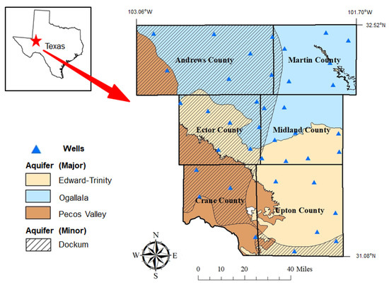
Figure 1.
The map of our study area showing county names, well locations, and aquifer types.
The alluvium overlies older Permian, Triassic- and Cretaceous- age rocks. It mostly consists of unconsolidated or poorly cemented clay, sand, gravel, and caliche. The Dockum Aquifer is a minor aquifer that extends across Crane, Andrews, and Ector County. The composition included Triassic-age sediments from the Dockum group and is 610 m thick [9,10,11]. The formations of the Dockum group are the Cooper Canyon, Santa Rosa, Tecovas, and Trujillo Formations. It consists of alternating sandstones and shales, with layers of silt and mudstone. Our study area is geologically situated on the shelf margin between the Delaware Basin and the Central Basin Platform [10,11]. The Permian Basin is characterized by a diverse range of complex formations. The Avalon, Bone Spring, Canyon, Clear Fork, Devonian, Ellenberger, San Andres, Spraberry, Wolfcamp, and Yeso are all part of the Permian Basin. The Permian basin is filled with sedimentary rocks and sediments ranging from Cambrian to Quaternary. This study area is characterized by oil and natural gas production depths ranging from a few hundred feet to five miles below the surface.
3. Data and Methods
The water data used in this study was collected from the Texas Water Development Board (TWDB) and the United States Geological Survey (USGS), which are open and public databases provided by U.S. government agencies. All counties annually examine the quality of the water supplies and inform the results to the public. For this research, we utilized reports generated from the following counties: Andrews, Martin, Midland, Ector, Crane, and Upton. The reports provide yearly average levels of water pollution parameters: Arsenic (As), Uranium (U), Nitrate (NO3−), Chloride (Cl), Fluoride (F), and total dissolved solids (TDS). The TDS is the mass of leftover materials after the evaporation. We obtained all historically available data from TWDB-USGS within the study area and verified the water wells locations based on their latitude and longitude coordinates. The Safe Water Drinking Act (SWDA) was implemented to ensure the safety of drinking water for everyone in the US. The EPA is responsible for establishing the maximum contaminant levels (MCLs) for drinking water quality and supervising water consumers who adhere to these guidelines. The Texas Commission of Environmental Quality (TCEQ) also implements standards to ensure water quality protection.
The parameters utilized for this research include Arsenic (As), Uranium (U), Nitrate (NO3−), Fluoride (F), Chloride (Cl), and TDS. The selected parameters in our study are necessary to present a long-term dataset with a condensed observation of the hydrological network [12]. Additionally, if you consume Arsenic (As), Uranium (U), and Nitrate (NO3−) at high concentrations, there could be some serious health issues that come with it [12,13,14,15,16]. Arsenic (As), Uranium (U), and Nitrate (NO3−) are classified as primary MCL, while Fluoride (F), Chloride (Cl), and TDS are considered secondary MCL. Primary MCLs are mandatory to follow, and the particular reason for circumstance is that the contaminants are proven to be the most detrimental to human health. While secondary MCLs are implemented mainly for aesthetic reasons, such as cloudy appearance or colors in the water, they affect the taste and smell of the water as well [17]. Secondary MCLs are not mandatory to follow and are only voluntarily tested because they do not pose a serious health risk. Nevertheless, even if the water is safe to drink, people may not want to drink cloudy, colored, or poor-tasting water. We collected all historically available data in the study area and checked the groundwater quality parameters from the Texas Water Development Board (TWDB), which is an open database provided by the US government. To understand the historical distribution of groundwater quality, we need long-term data with a relatively dense observation network for the groundwater parameters. Because of its relatively long-term data and availability of groundwater quality, we selected these parameters to evaluate the presence of inorganic and brackish contaminants in the Permian Basin, Texas. In terms of organic carbon matters, alkalinity, and pH, we found many missing historical data from TWDB.
For comparing the historical variations in water quality, data from 1992 to 2005 was correlated with data from 2006 to 2019. The values from Table 1 come from the TWDB and USGS reports, and the values from Table 2 and Table 3 are the contaminant averages calculated from each county. The report had many of the significant wells verified, and the selected data was collected from wells that were verified throughout the observation periods. A total of 481 observation samples (from thirty-seven wells) were obtained for this research. Reports were analyzed in Edwards-Trinity, Ogallala, Pecos Valley, and Dockum Aquifer from 1992 to 2005 and 2006 to 2019. Ector was the only county without any data from 1992 to 2005. Tables and figures were created by calculating the average of the aquifer contamination levels of each parameter throughout the years and were analyzed for temporal changes within the study area. The data was then compared to the EPA safety guidelines for each parameter, and conclusions were described about the water quality for each county.

Table 1.
Summary of selected well dataset in our study area.
Table 2.
Average pollutant levels from 1992 to 2005 (N/A: not available).
Table 3.
Average pollutant levels from 2006 to 2019 (N/A: not available).
Precipitation levels are important factors to evaluate groundwater environmental quality. For example, in our study, decreased precipitation may experience reduced recharge of aquifers, leading to lower groundwater levels. This can lead to the concentration of contaminants in the groundwater. When there is less water to dilute contaminants, their concentrations in the groundwater can increase. This effect is particularly pronounced in areas where groundwater is already contaminated with pollutants like nitrates or chloride. Additionally, the water table drops can lead to the mobilization of naturally occurring contaminants in the aquifer, such as arsenic or TDS, which may have been previously immobile in the presence of groundwater.
4. Results
4.1. Arsenic
Arsenic (As) is an element that appears naturally in sediments, soils, and rocks. It is utilized in industries such as mining, agriculture, and petroleum production. Arsenic is an extremely toxic material that is usually found in the natural world. Arsenic enters groundwater through rocks or can be introduced via activities like mining, agriculture, and industry, leading to the deposition of arsenic into water systems. It can contaminate the water via the process of hydraulic fracturing and horizontal drillings or via hydrocarbon releases. The harmful effects of arsenic on human health are serious. Exposure can cause skin damage, circulatory problems, and cancer [7]. Most of the arsenic that is found in public water systems comes from rock formations, but human activities such as agriculture and mining can deposit arsenic in groundwater [7,14]. In previous research, arsenic has been monitored at approximately 0.2 mg/L, a concentration much higher than what was observed in this research and exceeds the MCL [17,18]. Arsenic can be broadly distributed throughout the Earth’s crust, and it is highly likely to be found as arsenate/As(V) in water with a 5-oxidation state [7,14]. In situations of reduction, it is more expected to be observed as arsenite/As(III) in a 3-oxidation state [17].
Agriculture releases thousands of pounds of arsenic into the environment. Arsenic remains in the environment for a long time period [18]. Rodriguez et al. conducted a study over inorganic contaminants in the cities of Midland and Odessa, and other potential inputs for the contamination of arsenic in drinking water come from hydrocarbon releases [19]. When the hydrocarbons are released, the hydrocarbons can create a reduction in the environment, allowing for the mobilization of the contaminant. Likewise, Brown et al. [14] in 2010 led a study on the natural attenuation occurring arsenic at hydrocarbon-impacted regions where they noted that in sites with naturally occurring arsenic or an aged anthropogenic source, the background level will naturally exceed the MCL and obtaining below that remediation goal will be unachievable. The study also notes other constituents that could lead to arsenic contamination, such as agricultural activities and waste disposal. In addition, Hudak [7] conducted a study in 2010 on the arsenic, nitrate, and selenium levels in the Pecos Valley aquifer. In the study, he found that concentrations of arsenic were substantially higher in shallower wells and that the possible cause of contamination was from natural sources and agricultural activity. The dangers of consuming arsenic can increase the risk of long-term health issues; some of these health issues include circulatory disorders and various forms of bladder, kidney, and skin cancers [7,14].
When comparing this study to the other studies, the arsenic levels are still high enough for concern. Figure 2 demonstrates the average contamination levels of arsenic in each county using the data from Table 2 and Table 3. The highest levels of arsenic come from the Ogallala aquifer in Andrews and Martin Counties, where contamination levels reached 0.063 mg/L in Andrews and 0.05 mg/L in Martin (1992–2005). These contamination levels took place in northeast Martin County and northeast to southeast in Andrews County. Water quality in the area has not been improved vastly, with the average contamination levels in Martin at 0.018 mg/L and Andrews at 0.02 mg/L (1992–2005) to 0.017 mg/L in Martin and 0.016 mg/L in Andrews (2006–2019). Both of these counties still exceed the MCL for arsenic in their areas, which is set to 0.01 mg/L by the EPA [17].
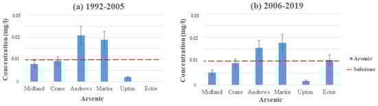
Figure 2.
Arsenic levels throughout the Permian Basin from (a) 1992–2005 and (b) 2006–2019.
4.2. Uranium
Uranium (U) naturally appears in soil, rocks, and water in the form of minerals [12,13]. In some cases, its appearance in the environment has to do with human impacts such as agriculture, mining, and petroleum production. Uranium can enter into a water body through rocks and soil that have Uranium or from mining, agricultural activities, and petroleum production. Bjørklund et al. [13] conducted a study on uranium in drinking water. The study notes that phosphate fertilization is a known source of uranium contamination in agricultural activities because of the phosphates applied to fertilizer production. According to the EPA [17], uranium is associated with hydraulic fracturing, where they state that “fracking” has changed the oil and gas profiles in terms of radioactivity produced. There was a significant positive association between uranium and nitrate, both parameters that are used in agriculture. The impacts uranium exposure has on human health have been studied extensively. Chronic exposure to uranium has a risk of long-term health effects; some of these may include cancer or kidney disease, leading to kidney inflammation and changes in urine composition, which can cause acute renal failure and death [15,16].
In the counties observed in this study, there was no available data for uranium contamination from 1992 to 2005. Uranium only appeared in the data from 2006 to 2019. Although Uranium does not exceed the EPA’s MCL in the data above, there were still a few wells in each county that did exceed the standard and are not shown in the data presented. Figure 3 displays the average contamination levels of each county for uranium using the data from Table 2 and Table 3. The highest contamination levels for Uranium also come from the Ogallala aquifer in Martin County, with levels reading 0.043 mg/L (2006–2019). These readings dramatically exceed the MCL for Uranium, which is set to 0.03 mg/L by the EPA [17]. There is no way to study temporal changes for uranium because there is no available data from (1992–2005). The reason for high contamination levels in Martin County is from manufactured fertilizers used on the land from agricultural activities.
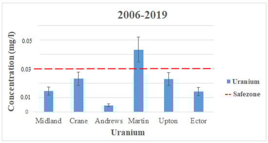
Figure 3.
Uranium levels throughout the Permian Basin from 2006–2019 (the observation period for 1992–2005 is not available from USGS).
4.3. Nitrate
Nitrate (NO3−) is a naturally occurring compound that has many human-made sources [7,16,20,21]. Nitrate forms from the nitrogen (N) element. Nitrogen (N2) gas is ~78% of the Earth’s atmospheric composition. In terms of the nitrogen cycle, nitrate is produced via the nitrification process, in which soil bacteria convert nitrogen dioxide (NO2) into ammonia (NH3). Subsequently, other soil bacteria introduced an oxygen atom to create nitrate. The process works full circle via the denitrification process under reducing conditions to convert from nitrate back to nitrogen gas. Nitrate is essential for all life and is commonly found in surface or groundwater, where it will not cause humans harm. However, high concentrations of nitrate in drinking water can lead to health issues. Nitrate is the result of human activities, including agriculture, septic systems, and farming. Children are more sensitive to high levels of nitrate than adults. After consuming groundwater with high levels of nitrate, the children can develop respiratory problems that can risk their lives. High levels of nitrate in groundwater occur from overuse of chemical fertilizers in agricultural, improper well locations [16,21]. Nelson et al. conducted a study on the assessment of environmental parameters with human activities in the Permian Basin, and Rodriguez et al. both agree that the contamination of groundwater from nitrate comes from inorganic fertilizers [12,19]. In addition, Reeves et al. [20] led a study on the chloride, dissolved solids, and nitrate concentration in the Ogallala aquifer. The research found that high nitrate contamination over 45 mg/L occurs in areas that are heavily cultivated, so to suspect that nitrogen-based fertilizers are the cause.
Figure 4 and Figure 5 represent the average contamination levels for nitrate in each county using the data from Table 2 and Table 3. The highest level of contamination comes from the Pecos Valley and Ogallala aquifers in Andrews and Martin County, with average contamination levels reading 48.8 mg/L in Martin County (1992–2005) and 40.25 mg/L in Andrews County (2006–2019). Both of these readings exceed the MCL for nitrate, which the EPA has set to 10 mg/L [17]. Martin water quality has improved a little bit, with its average contamination level at 32.4 mg/L (2006–2019), still exceeding the MCL set by the EPA. Andrews County contamination levels have become significantly worse, with the initial average level reading at 7.45 mg/L (1992–2005). In both of these counties, high concentration levels of nitrate come from inorganic nitrate fertilizers used on agricultural land [20]. Additionally, the well depth of the Ogallala is an underlying factor for contamination in these areas. As shallower wells are detected to have the highest levels of contaminants, the Ogallala aquifer is situated as low as 39 feet in depth.
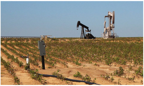
Figure 4.
Agricultural and oil field land in Ector County, the Permian Basin.
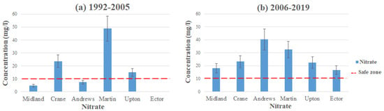
Figure 5.
Nitrate levels in Martin County from (a) 1992–2005 and (b) 2006–2019.
4.4. Fluoride
Fluoride (F) is an easily occurring material in nature. It can occur naturally in groundwater via geological compositions of soil and bedrock. However, it can also enter a water system from human activities such as industrial emissions, pesticides, and pharmaceuticals [22,23,24,25]. It is important for the maintenance of our teeth and bones. Nonetheless, there could still be a small chance of concern depending on the concentration of intake and the susceptibility of the individual [23]. Fluoride is considered a secondary MCL; therefore, it is not mandatorily enforced, but it is up to each individual county to enforce it. The highest level of fluoride concentration comes from the Edwards-Trinity and Pecos Valley aquifers in Ector County, with a concentration level of 9.31 mg/L exceeding the MCL, which is set to 4 mg/L by the EPA [17].
Figure 6 displays the average contamination levels of fluoride in each county using the data from Table 2 and Table 3. For Ector County, it was not possible to study temporal changes since it has no available data from (1992–2005). We could, however, study temporal changes for Andrews and Martin County, as they had the highest average concentration of fluoride, with Andrews reading at 2.83 mg/L and Martin at 3.3 mg/L (1992–2005), both remaining under the MCL. However, both counties had an increase in concentration (2006–2019), where Andrews average concentration levels were at 3.14 mg/L and Martin at 3.6 mg/L, yet still remaining under the MCL. The reason for the increase in concentration in both areas could be from a decrease in precipitation. Typically, regions with low levels of precipitation usually have a higher fluoride concentration compared to regions with higher levels of precipitation [18,23]. Hudak et al. [23] conducted a study in 2009 on elevated fluoride in West Texas groundwater, and they mentioned that about ~19% of fluoride concentration levels exceeded the MCL and that the levels were particularly higher in the southern part of the area. The study also states that although human activity may have an effect on fluoride levels, it is the natural sources that mainly account for the patterns monitored. However, for Ector County, Nelson et al. [12] stated that the reason for the high concentration levels is from a cement production facility located southwest in the county (Figure 7). Fluorspar is a common substance used in industrial cement [18,25]. Infiltration and runoff from these materials have led to the high concentrations detected in the area.
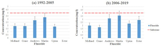
Figure 6.
Fluoride levels throughout the Permian Basin (a) 1992–2005 and (b) 2006–2019.
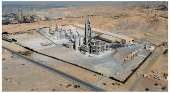
Figure 7.
Aerial images of the cement industry in our study area (from Google Earth).
4.5. Chloride
Chloride (Cl) occurs naturally and has the property of solubility in water. It exists in all natural waters, although its presence is usually at low concentrations. High levels of chloride can make water taste unpleasant, imparting a stronger salty flavor [20,26,27,28]. The high concentrations of chloride in the groundwater within our study area can be a potential hazard to the environment. The MCL for chloride in public water systems is 250 mg/L [17]. Chloride is a secondary MCL; therefore, it is not mandatorily enforced, and the standard is mainly applied for aesthetic reasons.
Figure 8 shows the average contamination levels of chloride in each county using the data from Table 2 and Table 3. The highest concentrations levels of chloride can be found in the southeastern part of Crane County, with the average concentration level reading 845.43 mg/L (1992–2005), way exceeding the MCL. Andrews and Martin follow after Crane with having the highest average concentrations, with Andrews reading at 436.4 mg/L and Martin at 472.9 mg/L (2006–2019), both exceeding the MCL. These high-level readings come from farmland development and the contamination related to cultivated crop production. Hudak [26] conducted a study in 2000 on chloride concentrations in Texas aquifers. The study concluded that high concentrations came from the mineral composition of the aquifers, seepage of saline water from other formations, and oil/gas production. Likewise, Reeves et al. conducted a study on dissolved solids and chloride concentrations in the Ogallala aquifer. The high concentrations of chloride come from a long-term vertical migration of saline water from cretaceous aquifers [20]. Additionally, Nelson et al. stated that the Ogallala and Pecos Valley aquifers’ depth in the area is not deep, allowing chloride to slip through the subsurface simply [12,20]. Between the two time intervals, it seems that the concentrations were lowered. The average level of chloride in Crane County is observed at 607.5 mg/L, Andrews at 417 mg/L, and Martin at 412 mg/L (2006–2019), but all three counties still exceed the MCL standard set by the EPA. Although chloride itself poses a small threat to human health, if ingested at abnormally high concentrations, it could cause a multitude of symptoms, including high blood pressure, fluid retention, spasms, uneven heart seizures, and rates [18]. The high concentrations in the area could be from fluids related to the oil and gas production, which are mainly composed of sodium chloride and increased TDS concentration [29].
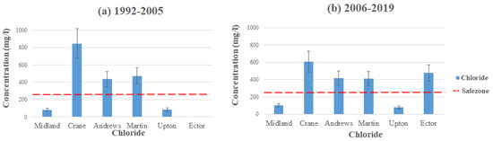
Figure 8.
Chloride levels throughout the Permian Basin from (a) 1992–2005 and (b) 2006–2019.
4.6. Total Dissolved Solids
Total dissolved solids (TDS) are the concentrations of combined inorganic salts and organic matter dissolved in water. Common inorganic salts found in groundwater include calcium, magnesium, potassium, and sodium [20,29,30,31,32]. These minerals can contaminate the groundwater from a few sources, both anthropogenic and natural activities. The increase in agricultural activities can result in high contamination levels of TDS in a given area. The harmful influences of TDS can affect taste and infrastructure, which occurs when concentration levels reach over 1000 mg/L in groundwater [33,34]. To avoid poor-tasting and cloudy water, it is advisable to keep the TDS level below 500 mg/L, which is the MCL set by the EPA [18,29].
Figure 9 displays the average contamination levels of TDS in each county using the data from Table 2 and Table 3. The highest concentration of TDS can be found in the southeastern part of Crane, with the average concentration reading 2762 mg/L (1992–2005) dramatically exceeding the MCL. Andrews and Martin follow after Crane in having the highest average concentration, with Andrews in the southern part of the county having 2351 mg/L and Martin in the northern part of the county at 1908 mg/L (1992–2005). These high concentration levels of TDS come from crop development, chemical fertilizers, and environmental changes in these areas. Elevated TDS concentration can also come from more natural causes, such as soil and rocks weathering in the subsurface [35,36,37]. However, Nelson et al. stated that the TDS levels began to rise when cropland started to develop [12,37]. The increased levels of TDS could result from the vegetation’s uptake of water, allowing soil to hold chlorides. Between the two time intervals, it seems that the concentration levels have gone down slightly, with Crane displaying 2382 mg/L, Andrews exhibiting 2307 mg/L, and Martin reducing to 1581 mg/L (2006–2019). Nonetheless, all three counties still exceed the MCL set by the EPA. TDS is considered a secondary MCL; therefore, it is not mandatory to follow and is mainly for aesthetic reasons. In addition, if consumed at abnormally high levels, it can cause nausea, lung irritation, vomiting, dizziness, etc. [38,39,40].
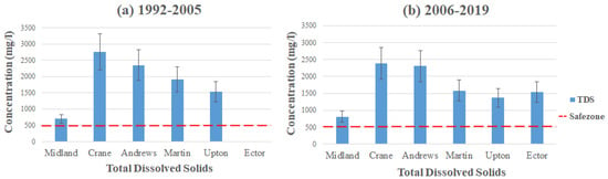
Figure 9.
Total dissolved solids level throughout the Permian Basin from (a) 1992–2005 and (b) 2006–2019.
5. Discussion
5.1. Groundwater with Population Growth
The population in the Permian Basin has significantly increased from the 1950s to 2020. In 1950, based on the US department of Commerce, the population census of Midland, Ector Crane, Upton, Martin, and Andrews County was at 83,410. However, in 2020, the population census in these counties was at 365,598, which is a 338% increase from the 1950s. The main reason for the population increase comes from oil- and gas-related opportunities in the area. With an increase in population comes an increase in human development. For example, in 1992, the total kilometers of developed land in Winkler County was at 145.3 km2, while in 2011, the developed land was at 280.4 km2, a 63% increase from 1992 [41,42]. The urbanization in these areas increases the runoff amount because of impervious areas in the developed land, leading to contamination in our aquifers [41]. The EPA’s primary groundwater regulations list all possible harmful effects from the long-term consumption of groundwater contaminants. Chloride can lead to liver issues and increases the danger of cancer. Fluoride can exist in groundwater at levels set by regulations, and continuous consumption can lead to bone disorders. TDS has no recorded human health effects, although these substances can alter the taste and visual characteristics of groundwater.
Anthropogenic activities such as oil and gas production have had a significant role in the contamination of soil because of brines and crude oil spills [43,44]. Spills could infiltrate the soil, resulting in water contamination, or alternatively, the contaminants could be emitted into the atmosphere [43]. Brines have a high TDS level of over 100,000 mg/L, and such high levels of TDS can include toxic trace components and naturally occurring radioactive substances such as uranium. With the development of drilling and hydraulic fracking, shales that were not previously feasible to drill are now recoverable. As a result, the amount of rigs in the study area increased to 500 at the end of 2011 [30,33]. Accordingly, more oil field facilities were established within the study area to account for the surge in production. This caused the land cover to change dramatically from 1992 to 2011, when the developed land’s amount expanded by ~12 km2, which is an increase of 178% [30]. Contamination of groundwater at oil and gas production sites comes from accidental discharges of drilling solutions, as well as refined and crude petroleum byproducts.
5.2. Climate Impact on Groundwater
Natural responses such as climate also play a role in the pollution of soil and groundwater. Figure 10 displays climate change within the Permian basin from 1980 to 2015. During this time, the total annual precipitation demonstrates a decreasing slope of −0.04, and the average rainfall was observed at 32.8 cm [30,33]. Based on the data displayed in Figure 10, our study area has an obvious decrease in precipitation and a significant increase in temperature, showing a shift to a more arid climate. Table 4 shows the trends in temperature and precipitation during the study period, 1980–2015. The coefficient of variation for annual total precipitation is 0.48, and the annual mean temperature is 0.04. The last value indicates that the study area had the smallest variation in annual mean temperature and exhibits a relatively even distribution. The significance test indicates statistically significant temperature trends at the 0.05 level. These results show that the study area is having a more prolonged drought, which causes an increase in soil stress. During these times of drought, fissures in the ground can form by an increase in effective stress from overlying strata, which in turn causes a migration pathway for pollutants to infiltrate groundwater [45,46].
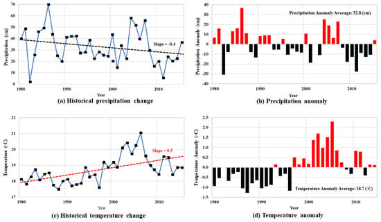
Figure 10.
Climate change in the Permian Basin during 1980-2015: (a) precipitation, (b) the anomalies, (c) temperature, and (d) the anomalies.
Table 4.
Annual climate data from 1980 to 2015.
Our results might suggest that the study area’s climate is gradually moving towards the more arid side of a semi-arid environment. As climate change continues, the growth in infiltration rates will also move ahead [31,47]. An escalation of severe drought conditions for our arid or semi-arid environments will expedite this process. The transition to drier and more drought-prone conditions changes groundwater conditions. Under drought events, vegetation dies off, leading to a decrease in ground cover, soil moisture absorption, and evapotranspiration. A shortage of precipitation reduces groundwater supplies and exacerbates the dehydration of surface soils. In conjunction with this finding, deterioration of groundwater quality was observed in the study area, suggesting the potential for further contamination in the future. Our research findings reveal that groundwater contamination within the Permian Basin results from a mix of human impacts and naturally prevailing environments. As the climate undergoes change, the impacts will become apparent in the reduction in recharge amounts. When this is coupled with anthropogenic activities, including agriculture, industry, and population developments, the deterioration of groundwater quality is accelerated.
6. Conclusions
Fresh groundwater in the Permian Basin is becoming increasingly scarce, which is why it is essential to conserve water. We collected and assessed public water contamination data from Andrews, Martin, Ector, Midland, Crane, and Upton Counties for the Dockum, Edwards-Trinity Plateau, Ogallala, and Pecos Valley aquifers from 1992 to 2019. The groundwater quality parameters looked at were arsenic, uranium, nitrate, fluoride, chloride, and total dissolved solids. We also identified temporal changes in the environments that affected water quality in the Permian Basin, Texas. When comparing the two time intervals of 1992–2005 and 2006–2019, in most cases, the contamination level was decreased but, nevertheless, still exceeded the MCL. Some factors that contribute to the contamination of these aquifers come from natural sources, aquifer depth, and anthropogenic activities such as agriculture and oil production. Based on the data collected for all aquifers, Andrews, Martin, and Crane Counties had consistently the highest contamination levels within the study area. Nitrate and total dissolved solids were the parameters that consistently exceeded the EPA’s maximum contaminant level. Human impacts such as oil spills, agriculture, and chemical fertilizers are major factors that contribute to the contaminants in the water. This research contributes to understanding the responses of groundwater quality associated with climate change (i.e., temperature increase and precipitation decrease) and human impacts (such as population growth, oil and gas developments, and urbanization). Therefore, this research can provide important information for water resources managers in making important decisions for the Permian Basin, Texas, and developing plans for the use of water resources in the future for a semi-arid and dry climate region. By combining these approaches, scientists and policymakers can gain a better understanding of how groundwater resources respond to human activities and climate change. This knowledge can inform sustainable water resource management and adaptation strategies to safeguard groundwater supplies for the future.
Collaboration between researchers, industry stakeholders, and government agencies is paramount. This multidisciplinary approach will also lead to the development of stringent regulations and best practices for industries such as oil and gas extraction, agriculture, and wastewater management. It is essential to identify the sources and pathways of contamination, as well as the specific contaminants involved. This will also provide a solid foundation for informed decision-making and targeted remediation efforts. Long-term solutions should focus on improving sustainable practices, including the adoption of remediation technologies, responsible land use, and improved water management strategies.
Author Contributions
J.H. designed the structure, developed the arguments, and contributed to the overall paper. J.L. collected detailed information about the water and calculated the contamination changes. N.R.R. analyzed the results and contributed to the overall paper. C.L. made critical revisions and contributed to the overall paper. All authors have read and agreed to the published version of the manuscript.
Funding
This research received no external funding.
Institutional Review Board Statement
Not applicable.
Informed Consent Statement
Not applicable.
Data Availability Statement
Data sharing not applicable.
Conflicts of Interest
The authors declare no conflict of interest.
References
- Bridget, S.; Robert, R.; Pei, X.; Mark, E.; Nicot, J.P.; David, Y.; Qian, Y.; Svetlana, I. Can we beneficially reuse produced water from oil and gas extraction in the U.S.? Sci. Total Environ. 2020, 717, 137085. [Google Scholar]
- Hopkins, J. Water-Quality Evaluation of the Ogallala Aquifer, Texas; Texas Water Development Board: Austin, TX, USA, 1993.
- Howell, N. Comparative Water Qualities and Blending in the Ogallala and Dockum Aquifers in Texas. Hydrology 2021, 8, 166. [Google Scholar] [CrossRef]
- Strause, J. Texas ground-water quality. US Geol. Surv. Open File Rep. 1987, 87, 0754. [Google Scholar]
- Fontenot, B.; Hunt, L.; Hildenbrand, Z.; Carlton, D.; Oka, H.; Walton, J.; Hopkins, D.; Osorio, A.; Bjorndal, B.; Hu, Q.; et al. An evaluation of water quality in private drinking water wells near natural gas extraction sites in the Barnett Shale Formation. Environ. Sci. Technol. 2013, 47, 10032–10040. [Google Scholar] [CrossRef]
- Hudak, P. Oil Production and Groundwater Quality in the Edwards-Trinity Plateau Aquifer, Texas. Sci. World J. 2003, 3, 167167. [Google Scholar] [CrossRef][Green Version]
- Hudak, P. Nitrate, arsenic and selenium concentrations in the Pecos valley aquifer, West Texas, USA. Int. J. Environ. Res. 2010, 4, 229–236. [Google Scholar]
- Hutchison, W. Edward-Trinity (Plateau), Pecos Valley and Trinity Aquifers: Nine Factor Documentation and Predictive Simulations. Groundw. Manag. Area 7 2016, 2, 1–14. [Google Scholar]
- Mace, R.; Angle, E. Aquifers of West Texas; Texas Water Development Board: Austin, TX, USA, 2001; Volume 356, pp. 1–272.
- Guru, M.; Horne, J. The Ogallala Aquifer; WIT Press: Southampton, UK, 1970; Volume 48. [Google Scholar]
- Bradley, R.; Sanjeev, K. The Dockum Aquifer in West Texas. In Aquifers of West Texas; Mace, R.E., Mullican, W.F., Angle, E.S., Eds.; Texas Water Development Board: Austin, TX, USA, 2001; p. 167174. [Google Scholar]
- Nelson, R.; Heo, J. Monitoring environmental parameters with oil and gas developments in the Permian Basin, USA. Int. J. Environ. Res. Public Health 2020, 17, 4026. [Google Scholar] [CrossRef]
- Bjørklund, G.; Semenova, Y.; Pivina, L.; Dadar, M.; Rahman, M.; Aaseth, J.; Chirumbolo, S. Uranium in drinking water: A public health threat. Arch. Toxicol. 2020, 94, 1551–1560. [Google Scholar] [CrossRef]
- Brown, R.; Patterson, K.; Zimmerman, M.; Ririe, G. Attenuation of Naturally Occurring Arsenic at Petroleum Hydrocarbon-impacted Sites. American Petroleum Institute (API). 2010. pp. 1–41. Available online: https://www.api.org/oil-and-natural-gas/environment/clean-water/ground-water/managing-arsenic-ingw (accessed on 1 June 2023).
- Cothern, C.; Lappenbusch, W. Occurrence of uranium in drinking water in the U.S. Health Phys. 1983, 45, 89–99. [Google Scholar] [CrossRef]
- Hudak, P. Associations between Dissolved Uranium, Nitrate, Calcium, Alkalinity, Iron, and Manganese Concentrations in the Edwards-Trinity Plateau Aquifer, Texas, USA. Environ. Process. 2018, 5, 441–450. [Google Scholar] [CrossRef]
- EPA (Environmental Protection Agency). Drinking Water Standard and Advisory Tables; EPA: Washington, DC, USA, 2018. Available online: https://www.epa.gov/dwstandardsregulations/2018-drinking-water-standards-and-advisory-tables (accessed on 5 July 2023).
- EPA (Environmental Protection Agency). Parameters of Water Quality—Interpretation and Standards Wellhead Protection; EPA: Washington, DC, USA, 2001. Available online: https://www.epa.ie/pubs/advice/water/quality/Water_Quality.pdf (accessed on 10 May 2023).
- Rodriguez, J.; Heo, J.; Park, J.; Lee, S.; Miranda, K. Inorganic pollutants in the water of Midland and Odessa, Permian Basin, west Texas. Air Soil Water Res. 2019, 12, 1–7. [Google Scholar] [CrossRef]
- Reeves, C., Jr.; Miller, W. Nitrate, Chloride and Dissolved Solids, Ogallala Aquifer, West Texas a. Groundwater 1978, 16, 167–173. [Google Scholar] [CrossRef]
- Wang, Y.; Ying, H.; Yin, Y.; Zheng, H.; Cui, Z. Estimating soil nitrate leaching of nitrogen fertilizer from global meta-analysis. Sci. Total Environ. 2019, 657, 96–102. [Google Scholar] [CrossRef]
- Fawell, J.; Bailey, K.; Chilton, J.; Dahi, E.; Fewtrell, L.; Magara, Y. Fluoride in Drinking Water; World Health Organization (WHO): Geneva, Switzerland, 2006. [Google Scholar]
- Hudak, P. Elevated fluoride and selenium in west Texas groundwater. Bull. Environ. Contam. Toxicol. 2009, 82, 39–42. [Google Scholar] [CrossRef] [PubMed]
- Meenakshi, R.; Maheshwari, C. Fluoride in drinking water and its removal. J. Hazard. Mater. 2006, 137, 456–463. [Google Scholar] [CrossRef]
- Qunitero, N. Examining the Use of Fluorspar in the Cement Industry. CEMEX Research Group. 2013. Available online: https://www.cemex.com (accessed on 10 April 2023).
- Hudak, P. Sulfate and chloride concentrations in Texas aquifers. Environ. Int. 2000, 26, 55–61. [Google Scholar] [CrossRef] [PubMed]
- Hudak, P. Solute distribution in the Ogallala Aquifer, Texas: Lithium, fluoride, nitrate, chloride and bromide. Carbonates Evaporites 2016, 31, 437–448. [Google Scholar] [CrossRef]
- Zhang, M.; Harrington, P. Determination of Trichloroethylene in Water by Liquid–Liquid Microextraction Assisted Solid Phase Microextraction. Chromatography 2015, 2, 66–78. [Google Scholar] [CrossRef]
- Devesa, R.; Dietrich, A. Guidance for optimizing drinking water taste by adjusting mineralization as measured by total dissolved solids (TDS). Desalination 2018, 439, 147–154. [Google Scholar] [CrossRef]
- Rodriguez, J.; Heo, J.; Kim, K. The impact of hydraulic fracturing on groundwater quality in the Permian Basin, west Texas, USA. Water 2020, 12, 796. [Google Scholar] [CrossRef]
- Haskell, D.; Heo, J.; Park, J.; Dong, C. Hydrogeochemical evaluation of groundwater quality parameters for Ogallala aquifer in the southern High Plains region, USA. Int. J. Environ. Res. Public Health 2022, 19, 8453. [Google Scholar] [CrossRef]
- Pfister, S.; Capo, R.C.; Stewart, B.W.; Macpherson, G.L.; Phan, T.T.; Gardiner, J.B.; Diehl, J.R.; Lopano, C.L.; Hakala, J.A. Geochemical and lithium isotope tracking of dissolved solid sources in Permian Basin carbonate reservoir and overlying aquifer waters at an enhanced oil recovery site, northwest Texas, USA. Appl. Geochem. 2017, 87, 122–135. [Google Scholar] [CrossRef]
- EPA (Environmental Protection Agency). Hydraulic Fracturing for Oil and Gas: Impacts from the Hydraulic Fracturing Water Cycle on Drinking Water Resources in the United States. 2016. Available online: https://cfpub.epa.gov/ncea/hfstudy/recordisplay.cfm?deid=332990 (accessed on 20 June 2023).
- Long, S. Direct and indirect challenges for water quality from the hydraulic fracturing industry. Am. Water Work. Assoc. 2014, 106, 53–57. [Google Scholar] [CrossRef]
- Mehany, M.; Kumar, S. Analyzing the feasibility of fracking in the U.S. using macro level life cycle cost analysis and assessment approaches—A foundational study. Sustain. Prod. Consum. 2019, 20, 375–388. [Google Scholar] [CrossRef]
- Meng, Q. The impact of fracking on the environment: A total environmental study paradigm. Sci. Total Environ. 2017, 580, 953–957. [Google Scholar] [CrossRef] [PubMed]
- Carls, E.; Fenn, D.; Chaffey, S. Soil contamination by oil and gas drilling and production operations in Padre Island national seashore, Texas, USA. J. Environ. Manag. 1995, 45, 273–286. [Google Scholar] [CrossRef]
- Taylor, M.; Elliott, H.; Navitsky, L. Relationship between total dissolved solids and electrical conductivity in Marcellus hydraulic fracturing fluids. Water Sci. Technol. 2018, 77, 1998–2004. [Google Scholar] [CrossRef]
- Ajemigbitse, M.; Tasker, T.; Cannon, F.; Warner, N. Influence of High Total Dissolved Solids Concentration and Ionic Composition on γ Spectroscopy Radium Measurements of Oil and Gas-Produced Water. Environ. Sci. Technol. 2019, 53, 10295–10302. [Google Scholar] [CrossRef]
- Standen, A.; Opdyke, D. Contamination Migration, Characteristics, and Responses for the Edwards–Trinity Plateau Aquifer. Aquifers Edw. Plateau Tex. Water Dev. Board 2004, 360, 211–234. [Google Scholar]
- EIA (Energy Information Administration). Annual Energy Review 2011; EIA U.S. Department of Energy: Washington, DC, USA, 2012. Available online: https://www.eia.gov/totalenergy/data/annual/pdf/aer.pdf (accessed on 15 May 2023).
- Bradley, R.; Sanjeev, K. The Dockum aquifer in the Edwards Plateau. Aquifers Edw. Plateau Tex. Water Dev. Board Rep. 2004, 360, 149–164. [Google Scholar]
- Neville, P.; Coward, R.; Watson, R.; Inglis, M.; Morain, S. The application of TM imagery and GIS data in the assessment of arid lands water and land resources in west Texas. Photogramm. Eng. Remote Sens. 2000, 66, 1373–1379. [Google Scholar]
- Amariah, F.; Matthew, S. Water, culture, and adaptation in the High Plains-Ogallala Aquifer region. J. Rural Stud. 2022, 95, 195–207. [Google Scholar]
- Dutton, A.; Raney, J. Review of data on hydrogeology and related issues in Andrews County, Texas. In Bureau of Economic Geology; The University of Texas at Austin: Austin, TX, USA, 1999; pp. 1–16. [Google Scholar]
- Thurman, E.; Bastian, K.; Mollhagen, T. Occurrence of cotton herbicides and insecticides in playa lakes of the High Plains of West Texas. Sci. Total Environ. 2000, 248, 189–200. [Google Scholar] [CrossRef] [PubMed]
- Anandhi, A.; Deepa, R.; Bhardwaj, A.; Misra, V. Temperature, Precipitation, and Agro-Hydro-Meteorological Indicator Based Scenarios for Decision Making in Ogallala Aquifer Region. Water 2023, 15, 600. [Google Scholar] [CrossRef]


Disclaimer/Publisher’s Note: The statements, opinions and data contained in all publications are solely those of the individual author(s) and contributor(s) and not of MDPI and/or the editor(s). MDPI and/or the editor(s) disclaim responsibility for any injury to people or property resulting from any ideas, methods, instructions or products referred to in the content. |
© 2023 by the authors. Licensee MDPI, Basel, Switzerland. This article is an open access article distributed under the terms and conditions of the Creative Commons Attribution (CC BY) license (https://creativecommons.org/licenses/by/4.0/).