4.3. Configuration Results
In the first tier of the optimization strategy, the IES shifts to silo operation in the face of extreme events, and the best configuration investment plan is found by enhancing the redundancy of the installed size and adjusting the supply structure of energy coupling equipment and energy supply devices.
In this paper, due to the space limitation of the environmental area, the upper limit of the scale capacity of IES energy supply and energy coupling equipment Imax is set to 4 MW. Five different scenarios are formulated based on the parameter settings and priority objectives of the tolerant hierarchical sequence method to compare and analyze:
Scenario 1: With economy as the first priority target, the tolerance parameter ε setting for the resilience index is set to be 0.6 and a Markov decision process is used to go for energy supply regulation strategies.
Scenario 2: With economy as the first priority target, the tolerance parameter ε setting for the resilience indicator is set to be 0.2 and a Markov decision process is used to go for energy supply regulation strategies.
Scenario 3: With resilience as the first priority target, the tolerance parameter ε setting for economic indicators is set to be 0.8 and a Markov decision process is used to go for energy supply regulation strategies.
Scenario 4: With resilience as the first priority target, the tolerance parameter ε setting for economic indicators is set to be 0.4 and a Markov decision process is used to go for energy supply regulation strategies.
Scenario 5: With resilience as the first priority objective, the tolerance parameter ε for the economic indicators is set to 0.4. However, the Markov decision process energy supply regulation strategy is not used.
In MATLAB 2020b, a resilient economic two-tier optimization strategy, as well as the methodology proposed in this paper, is used to obtain the initial configuration of an islanded integrated energy system. The obtained energy coupling equipment configuration options are shown in the
Table 4.
Considering the three critical loads of electricity, heat, and cold, the amount of integrated energy system loss of load at each time point is derived, the time period with more load supply loss in IES decision-making is identified to readjust the energy supply allocation planning, and the energy supply structure and the parameters such as the installed capacity of the coupled equipment, the resilience tolerance, and the key loads are adjusted by continuous feedback iteration. Economic and resiliency indicators are shown in the
Table 5 and
Table 6.
From the results in the table, it can be seen that the choice of the first objective, and the tolerance setting of the secondary objective will seriously affect the results of the configuration of the supply coupling equipment for the islanded IES, and due to the constraints of the economic indicators and the amount of lost load, the total configuration size of the five scenarios for the islanded IES will basically be close to the maximum installed scale capacity of 4 MW.
Scenarios 4 and 5, the first objective of the selection of resilience indicators and economic cost tolerance settings are also the same, so the two scenarios of the annualized investment costs and the configuration of the energy supply coupling equipment to solve the same results, the difference between the two is that Scenario 5 does not use the Markov returns to assist in decision-making to regulate the supply of energy. From the typical day data, annualized operation, and maintenance and energy costs, in Scenario 5, IES energy supply equipment scheduling process, the IES center did not receive the return value of the scheduling strategy for the future time period, and only found that the new energy generation equipment cannot meet the load requirements after the hasty dispatch to meet the demand at that time, and cannot trade-off the overall economic cost of a typical day within 24 h and resilience goals. And scenario five will be the relationship between heating, power supply, and cooling separately, not fully utilizing the coupled equipment before the synergistic effect, resulting in energy supply equipment part of the time period of the phenomenon of excess power. Energy consumption is not used by the demand side, so that the waste of resources and the economic cost, and the annualized cost of operation and maintenance of the scenario four rose by 14.87%, and the annualized cost of energy consumption rose by 17.60%, reaching CNY 124.51 thousand. Meanwhile, the energy coupling conversion equipment is not fully utilized during the typical daily peak load demand hours in summer and winter, resulting in more lost loads than Scenario IV, with the typical daily resilience index in summer and the typical daily resilience index in winter being only 0.873 and 0.784, respectively. In Scenario IV, the Markov decision-making process-assisted regulation of the supply of energy makes the overall annualized cost of the IES fall by CNY 45.21 thousand, with a decline percentage of 5.24%. The good regulation strategy, which uses energy coupling equipment to charge when load demand is low and discharges during peak load consumption to achieve the effect of peak shaving and valley filling, improves the typical daily resilience indexes by 7.33%, 7.56%, and 13.01% in spring, summer, and fall, respectively, relative to Scenario 5. The first four scenarios all use a conditioning strategy with a Markov decision process. With the increasing weight on the resilience indicator load loss, the installed size of photovoltaic and electric boilers also tends to rise, because the output curve of photovoltaic is mostly in the daytime period of a typical day, which is roughly the same trend as that of the electric load curve, and the electric boiler with the elevated investment cost, but also can quickly convert electric energy into heat, which enhances the resilience of the winter heat supply. In Scenarios 1 and 2, the installed number of gas units and fan units is significantly higher than Scenarios 3 and 4, which may be caused by the higher cost of gas units and the fan in the middle of the night. There will be a certain degree of wind abandonment phenomenon of energy supply, and both scenarios in which the battery size is only 500 kW, which will soon be filled, and cannot be very good peak shaving to fill in the valley, result in a large amount of load loss enhancement. All four scenarios are solved by investing in a set of compression chillers.
It can be seen that in Scenario 1, where economy is the first priority goal, its total cost, investment cost, and energy consumption cost are less than Scenario 2, Scenario 3, and Scenario 4, and the total cost is decreased by 6.94%, 12.04%, and 15.77%, respectively, compared to Scenarios 2, 3, and 4, but its typical day resilience indexes are basically the worst performers of all four scenarios except for a better typical day in summer due to the configuration of the compression chillers and storage tanks, and the typical day in spring, fall, and winter with a spike in heat loads are poorly performed. The IES in the upper control will control the cost in the first place, and will not purchase enough heat storage tanks such as thermal energy storage and electric boilers, and due to the cost of too many gas-fired units subject to the limitations of the natural gas pipeline supply, it cannot be sufficient to supply the IES’ required heat. In contrast, Scenario 4 basically does not consider the cost aspects of the problem. The reasonable configuration of the ratio between the supply and coupling equipment, as far as possible configuration of electric heat and cold energy storage equipment, makes full use of the synergistic relationship between the PV and the fan before a typical spring and fall day; its resilience index is 0.994, and the loss of load is only a very considerable 4.51%, although on a typical winter day there is still a 12.92% combined loss of load. The resilience metrics and economic costs associated with continuing to invest in compression chillers and storage tanks clearly do not meet the tolerance requirements of Scenario 4, and the loss of load is within an acceptable range, where the IES energy supply capacity is utilized to its fullest potential.
4.4. Operation Analysis
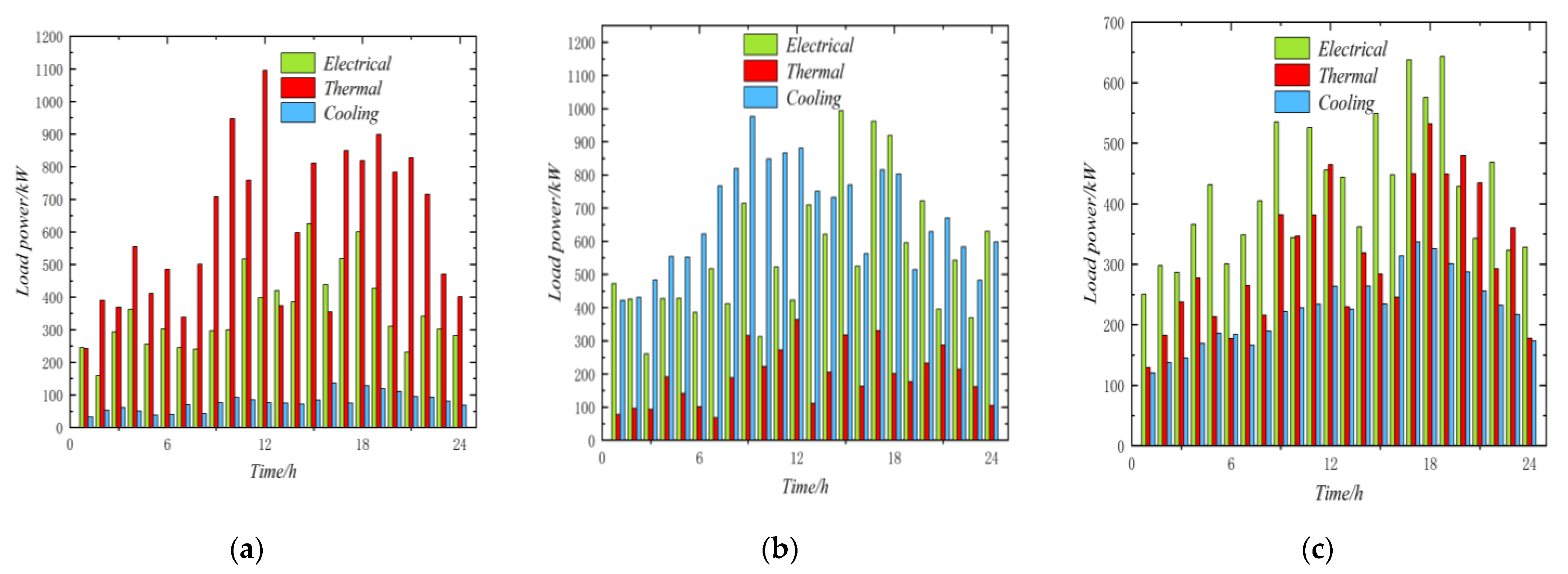
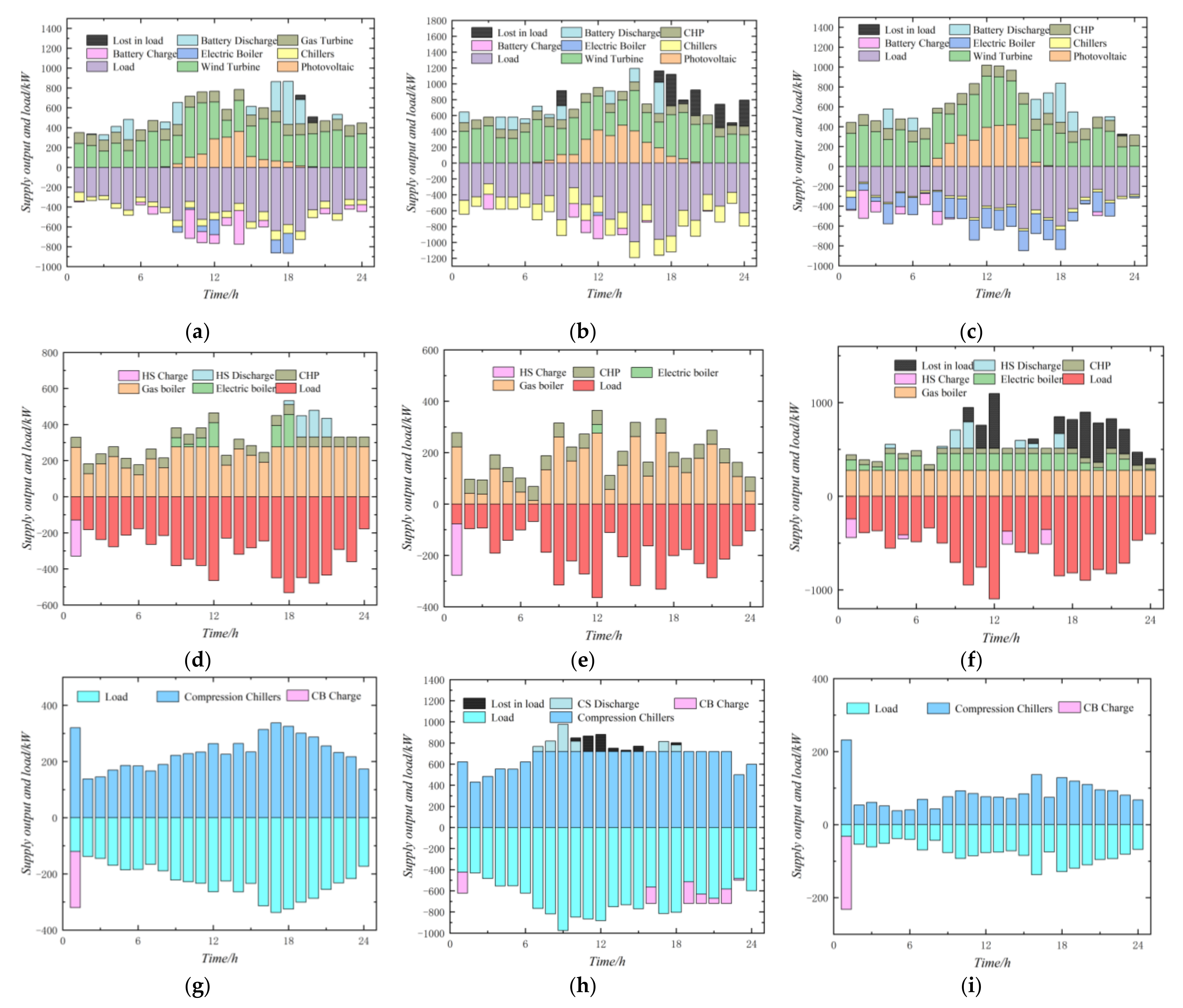
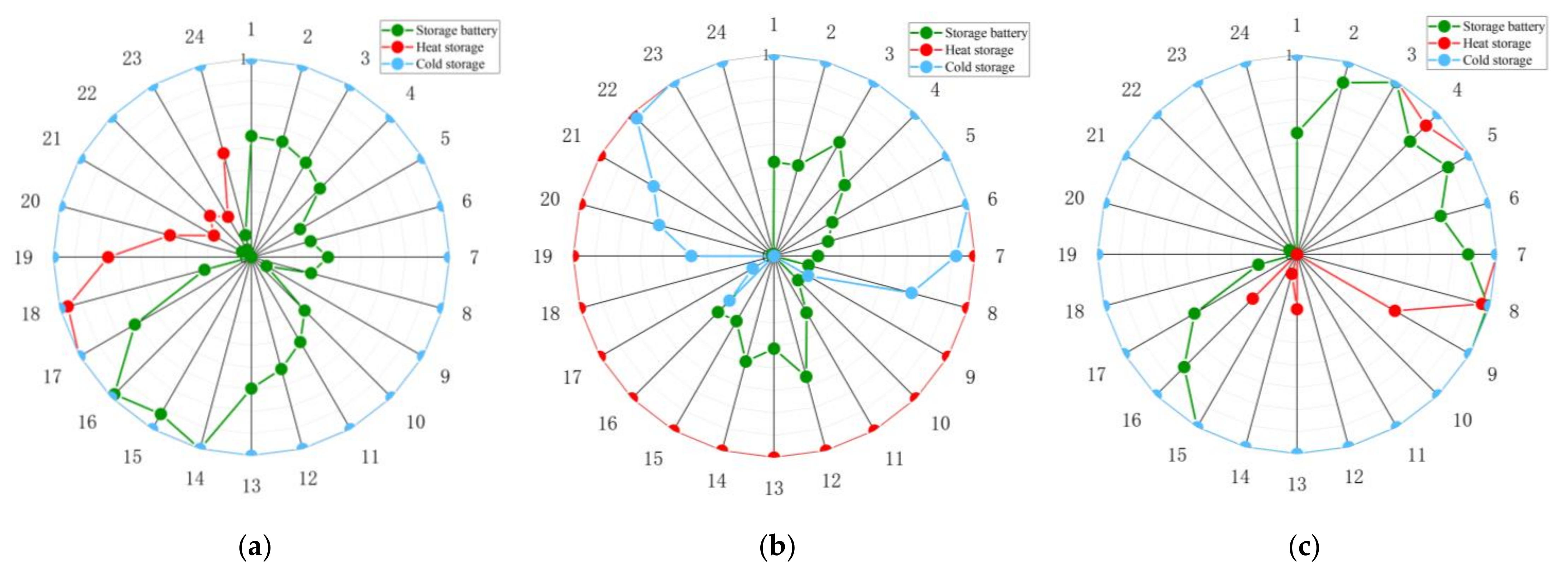
As an example, for Scenario 4, which has the greatest diversity in the types of energy-supply coupling equipment, the supply outputs and load profiles for each time period of the three typical days of the islanded integrated energy system are shown in
Figure 6 and
Figure 7 and
Table 7 and
Table 8.
On a typical day in spring and fall, the IES energy supply in the configuration of Scenario 4 is very effective, especially in the heating and cooling segments, where the IES perfectly supplies all the loads by utilizing relatively stable gas boilers, CHP units, and compression chillers. The cold storage tanks are not discharged on this typical day, and the heat storage tanks are only discharged from 19:00 to 22:00 h to balance the heat loads. In the power supply segment, the storage battery has more use; most of the time, it is involved in the IES energy supply, discharging at 4 to 6 o’clock and 14 o’clock to 19 o’clock, and recharging at 9 o’clock to 14 o’clock to maintain the battery operation, while the wind turbine, PV, and CHP as the main power supply most of the loads, and it can be seen that the wind turbine output is relatively smooth, and the trend of the PV output and the load curve have also similarities. The loss of load in the supply chain mainly comes from 19:00 to 21:00, which is a small amount of loss of load because there is almost no PV output in the IES, and the batteries have been depleted by the peak power consumption in the previous hours.
And when it comes to the simulation session on a typical summer day, the hot weather makes the demand of cold load rise sharply, and the cooling supply session is seriously challenged, the compression chillers are running at peak power from eight to 22 o’clock, and the power out of the remaining time period is higher than half of the rated maximum, and the saving cold tanks are supplying the cold by releasing from eight to ten o’clock, although the cold load is more than the maximum refrigeration capacity of the chillers, and the remaining capacity of the 500 kW storage tank was not enough to supply the cooling load until 11:00, and there was a cooling loss of 430.79 kW in the following six hours. The IES heating supply remained stable. At the height of summer, the usage of various electrical equipment rises sharply, plus the electric conversion of the compressed refrigeration machine also consumes a considerable portion of electricity, resulting in the irregularity of the IES electric load curve on a typical summer day. Although the fans, PV, and CHP units supply electricity stably, the irradiation intensity of the sun gradually becomes weaker from 17:00 to 24:00 when the sun goes down, and it is difficult for the fans and CHP units to support the full electric load, and the lost load totaled 4639.52 kW.
With lower temperatures in winter, the IES does not have much problem in both cooling and power supply on a typical day in winter, the loss of load in both power and cooling segments is zero with the synergistic effect of the multiple energy supply units and the energy coupling equipment. While facing a large number of lost loads from heat loads, due to the weighting of the IES economic indicators in addition to the resilience indicators in the process of solving the multi-objective using the tolerant hierarchical sequence method, it is taken into account that the lost loads only occur on typical winter days that only account for about a quarter of the year. Therefore, the installed capacity of the heating equipment includes only 300 lW gas boilers and 200 kW electric boilers, and the energy storage equipment has only 500 kW capacity, although the battery is charged and discharged by the Markov decision process to calm the heat load, the lack of the installed size allows the IES typical day in the morning and most of the evening to generate a large number of lost loads, and if you want to reduce the generation of lost loads, you can be in the tolerance setting parameter settings for appropriate cost reduction.


