Short- and Medium-Term Electricity Consumption Forecasting Using Prophet and GRU

Abstract

Electricity consumption forecasting plays a crucial role in improving energy efficiency, ensuring stable power supply, reducing energy costs, optimizing facility management, and promoting environmental conservation. Accurate predictions help optimize energy system operations, reduce energy wastage, cut costs, and decrease carbon emissions. Consequently, the research on electricity consumption forecasting algorithms is thriving. However, to overcome challenges like data imbalances, data quality issues, seasonal variations, and event handling, recent forecasting models employ various approaches, including probability and statistics, machine learning, and deep learning. This study proposes a short- and medium-term electricity consumption prediction algorithm by combining the GRU model suitable for long-term forecasting and the Prophet model suitable for seasonality and event handling. (1) The preprocessed data propose the Prophet model in the first step for seasonality and event handling prediction. (2) In the second step, seven multivariate data are experimented with using GRU. Specifically, the seven multivariate data consist of six meteorological data and the residuals between the predicted data from the proposed Prophet model in Step 1 and the observed data. These are utilized to predict electricity consumption at 15 min intervals. (3) Electricity consumption is predicted for short-term (2 days and 7 days) and medium-term (15 days and 30 days) scenarios. The proposed approach outperforms both the Prophet and GRU models, reducing prediction errors and offering valuable insights into electricity consumption patterns.

1. Introduction

The Building Energy Management System (BEMS) plays a pivotal role in managing the entire electricity system, encompassing power generation, transmission, distribution, and consumption. These systems employ energy management software, often implemented in contexts with high energy consumption like households, buildings, and factories. Their purpose is to meticulously analyze energy consumption concerning its source, heat generation, system operation, and major equipment utilization. By doing so, they aim to establish efficient energy management systems, thereby leading to cost savings through energy conservation, ensuring the appropriate usage of energy sources, reducing carbon emissions via optimal operation, decreasing facility operation and maintenance costs, extending equipment lifespan, and improving overall facility operation efficiency [1,2].

However, the true potential of BEMS can only be harnessed with reliable electricity consumption forecasting, especially in the short- and medium-term. Accurate forecasting in these timeframes is critical for energy system operations. It ensures a stable and reliable supply of power, optimizes resource allocation, and significantly contributes to overall energy efficiency. In this context, the accurate prediction of electricity consumption patterns becomes paramount [3]. Electricity consumption forecasting can be categorized into very short-term, short-term, medium-term, and long-term forecasts [4,5,6]. Very short-term electricity consumption forecasting predicts power consumption and demand in real-time, often making predictions for short intervals like 1 h, 15 min, and 30 min to ensure the stable operation of the power grid. Short-term electricity consumption forecasting covers predictions ranging from hourly forecasts to predictions over several weeks, achieved using algorithms such as Exponential Smoothing [7] and Auto-Regressive Integrated Moving Averages (ARIMA) [8]. Medium-term electricity consumption forecasting spans several weeks to months and leverages numerous variables such as meteorological data, event information, and economic indicators to predict power consumption. A variety of algorithms, such as linear regression, multiple regression, polynomial regression [9], neural networks [10], deep learning [11], and Long Short-term Memory (LSTM) [12], come into play. Long-term electricity consumption forecasting encompasses predictions spanning three months to a year, demanding consideration of more variables and system elements than short- and medium-term forecasts. Time-series analysis, ARIMA models, and ensemble techniques are often employed to discern trends and patterns of long-term power consumption.

While existing forecasting methods, like ARIMA and Exponential Smoothing, each have their strengths, they also face limitations. ARIMA excels at short-term forecasts but struggles with seasonality and non-stationarity in data, making long-term predictions challenging. Exponential Smoothing performs well for short-term forecasting but encounters difficulties when forecasting long-term trends and incorporating additional factors. The Prophet model suits medium-term forecasting with its ability to handle seasonality and events but finds long-term trend prediction challenging. LSTM is ideal for long-term forecasting, given its capacity to learn long-term dependencies in time-series data. However, it is sensitive to data quality and quantity and demands substantial computational resources for training and prediction [13,14,15].

Recent advancements in electricity consumption forecasting involve combining various techniques tailored to data characteristics and forecasting objectives [16,17,18,19,20,21,22,23,24,25]. For instance, the synergy between Prophet and LSTM has demonstrated improved accuracy and performance in short- and long-term electricity consumption predictions [16,17]. Similarly, studies have proposed combining ARIMA with XGBoost for short-term electricity consumption forecasting [18] and ARIMA with Bi-LSTM models for forecasting smart grid parameters [19]. Additionally, hybrid models like ARIMA-LSTM and ARIMA-GRU blend ARIMA for modeling trends and seasonality in time-series data with LSTM or GRU to enhance prediction performance [20,21]. It also emphasizes the importance of load and power demand prediction technology using hierarchical prediction models [22,23]. Furthermore, research efforts have delved into the usage of multivariate models, such as those based on multilayered LSTM [24] and ConvLSTM [25], to effectively manage complex time-series data. While these studies have assessed the strengths, weaknesses, and performance of these models, the complexity of parameter configuration and the intricacies of the training process for these combined models can pose challenges. Moreover, their performance can be contingent on the application domain and data characteristics.

This study proposes a novel approach for short- and medium-term electricity consumption prediction by combining the GRU model, suitable for long-term forecasting, and the Prophet model, adept at capturing seasonality and events. The proposed methodology is summarized as follows:

(1)

Data Collection and Preprocessing: We gather electricity consumption data and meteorological data from Manufacturing Company B in Naju, Jeollanam-do, Republic of Korea. These datasets are meticulously preprocessed to ensure data quality.

(2)

Prophet Model for Seasonality: In the first step, we employ the Prophet model to address seasonality and events in electricity consumption. This step is crucial for understanding and predicting short-term fluctuations and patterns.

(3)

GRU Model for Multivariate Prediction: The second step involves utilizing the GRU model to predict electricity consumption at 15 min intervals. We experiment with seven multivariate datasets, including six meteorological variables and the residuals derived from comparing the data predicted by the Prophet model in Step 1 with the observed data.

(4)

Short- and Medium-Term Predictions: Our approach is tested for both short-term (2 days and 7 days) and medium-term (15 days and 30 days) electricity consumption predictions.

The study’s structure is as follows: Section 2 discusses related research on the Prophet and GRU models. Section 3 addresses the problems of the existing Prophet and proposes solutions. Section 4 explains the algorithm and experimental results of the proposed method. Finally, Section 5 concludes the study.

2. Related Works

2.1. Prophet Model

The Prophet model, an open-source time-series forecasting library developed by Facebook [26], stands as a robust solution for predicting time-series data with dynamic temporal changes. Its applicability spans across a wide array of domains, including marketing, advertising, demand projection, energy consumption forecasting, and financial prediction. The Prophet model is structured with three fundamental components, as represented by Equation (1).

Y(t) = g(t) + s(t) + h(t) + ε(t)

(1)

In Equation (1), y(t) signifies the observed value at the time point t. The component g(t) embodies the trend, elucidating the overarching long-term growth or decline trends within the time series. S(t) characterizes the seasonality component, adept at capturing recurrent patterns and oscillations. H(t) assumes the role of the holidays component, adeptly accounting for singular events or exceptional incidents that may influence the time series. Finally, ε(t) represents the error term, accommodating any stochastic or irregular variations present in the data. Prophet’s versatility and adeptness in accommodating diverse time series patterns make it an immensely popular and potent tool for time-series forecasting across a multitude of industries.

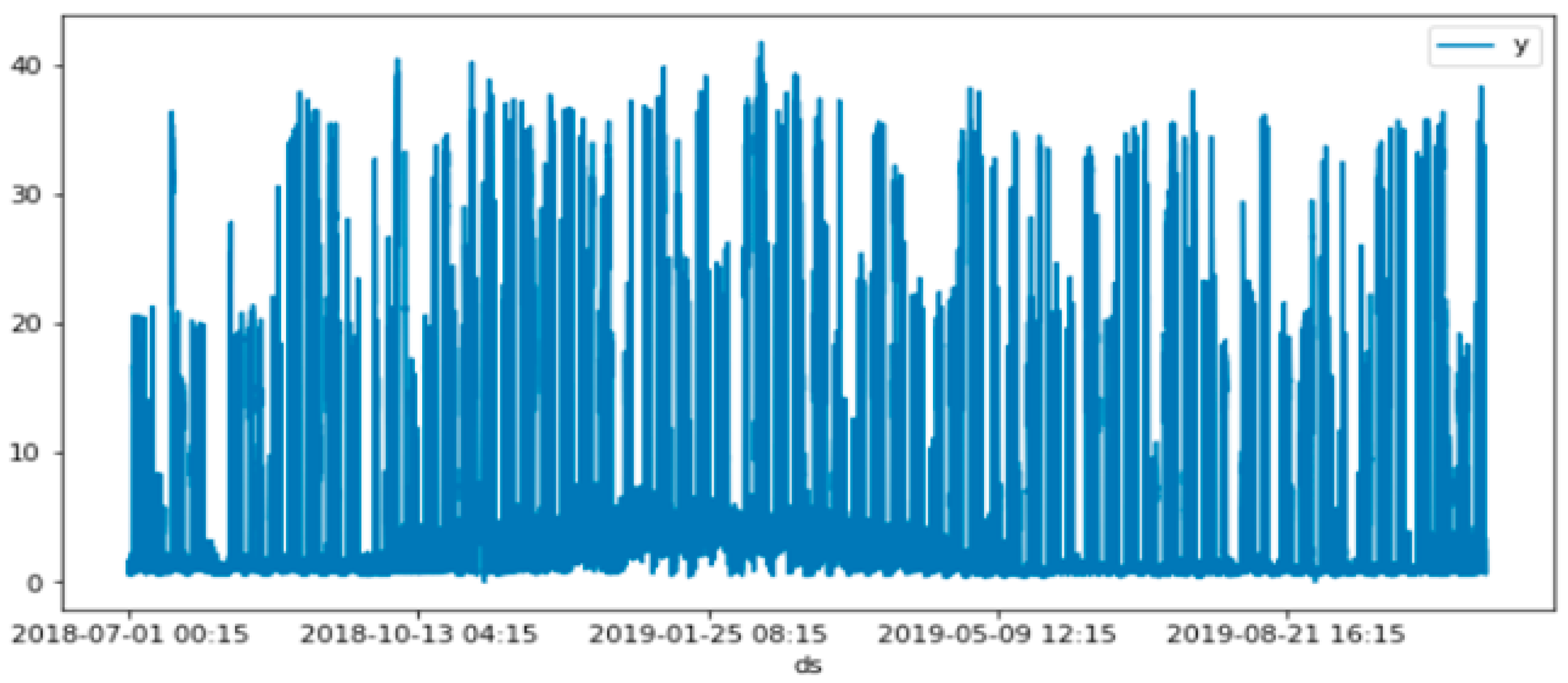
Figure 1 depicts the electricity consumption data of Company B collected from 1 July 2018 to 31 October 2019 in this study.

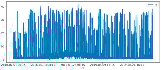
Figure 1. Electricity consumption data of Company B collected from 1 July 2018 to 31 October 2019.

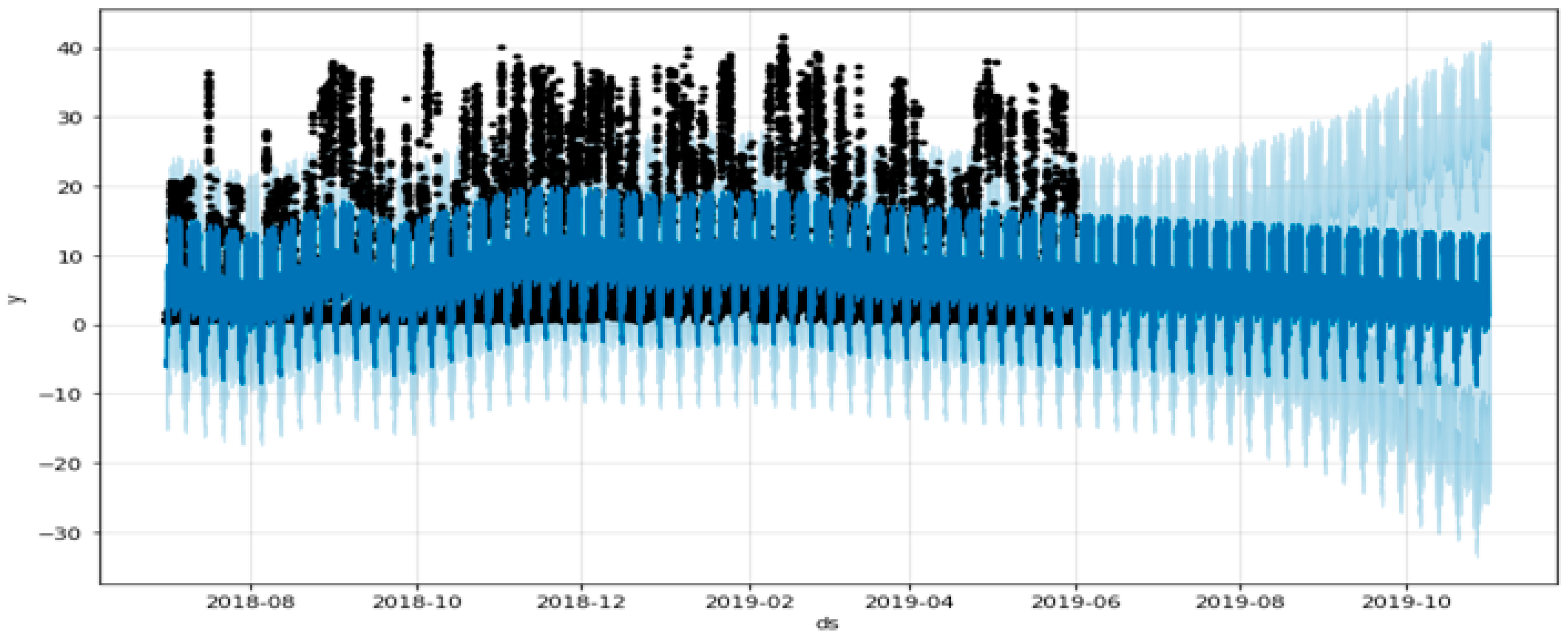
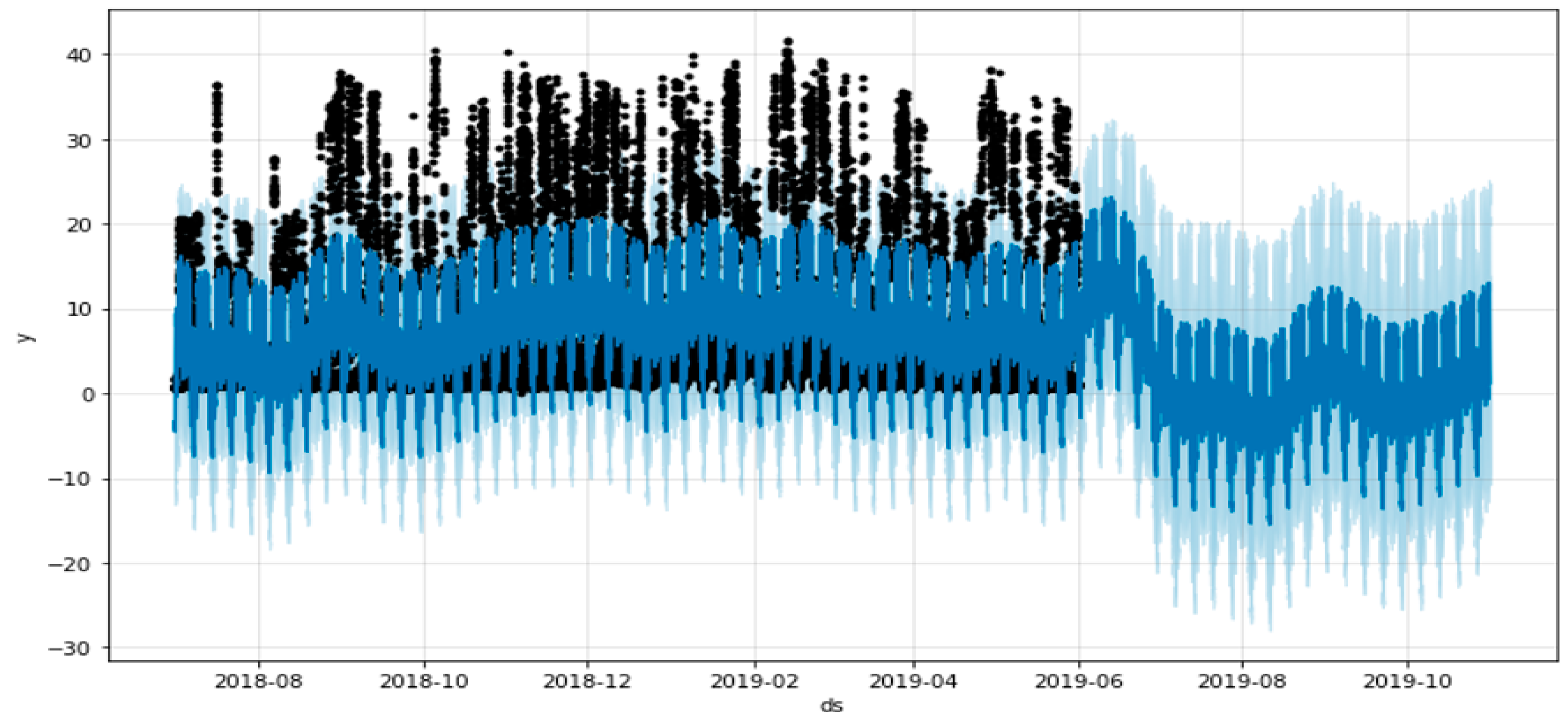
Figure 2 and Figure 3 illustrate the results of applying the basic Prophet model. The model was trained on one year of data from July 2018 to June 2019. In Figure 2, the black dots represent the observed data values from July 2018 to June 2019, while the dark blue line represents the model’s predicted values from July 2018 to October 2019. The light blue line indicates the uncertainty interval. Notably, the period up to June 2019 demonstrates the in-sample fit, where the model is fitted to the training data. Beyond that point, the out-of-sample forecast is depicted, representing predictions for the test data.

Figure 2. A basic Prophet model that only considers the holiday effect on the training data for one year (July 2018 to June 2019).

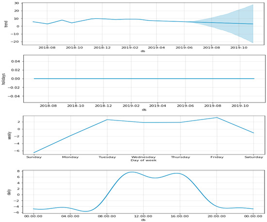
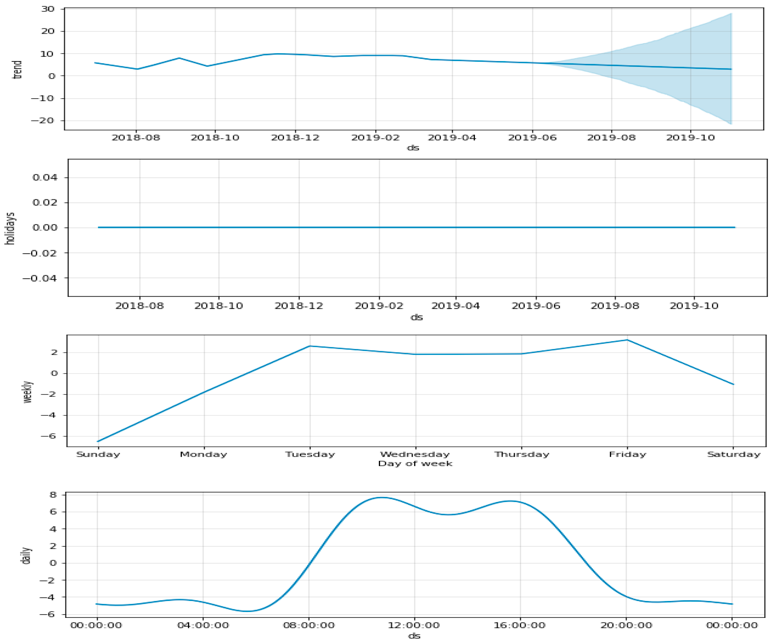
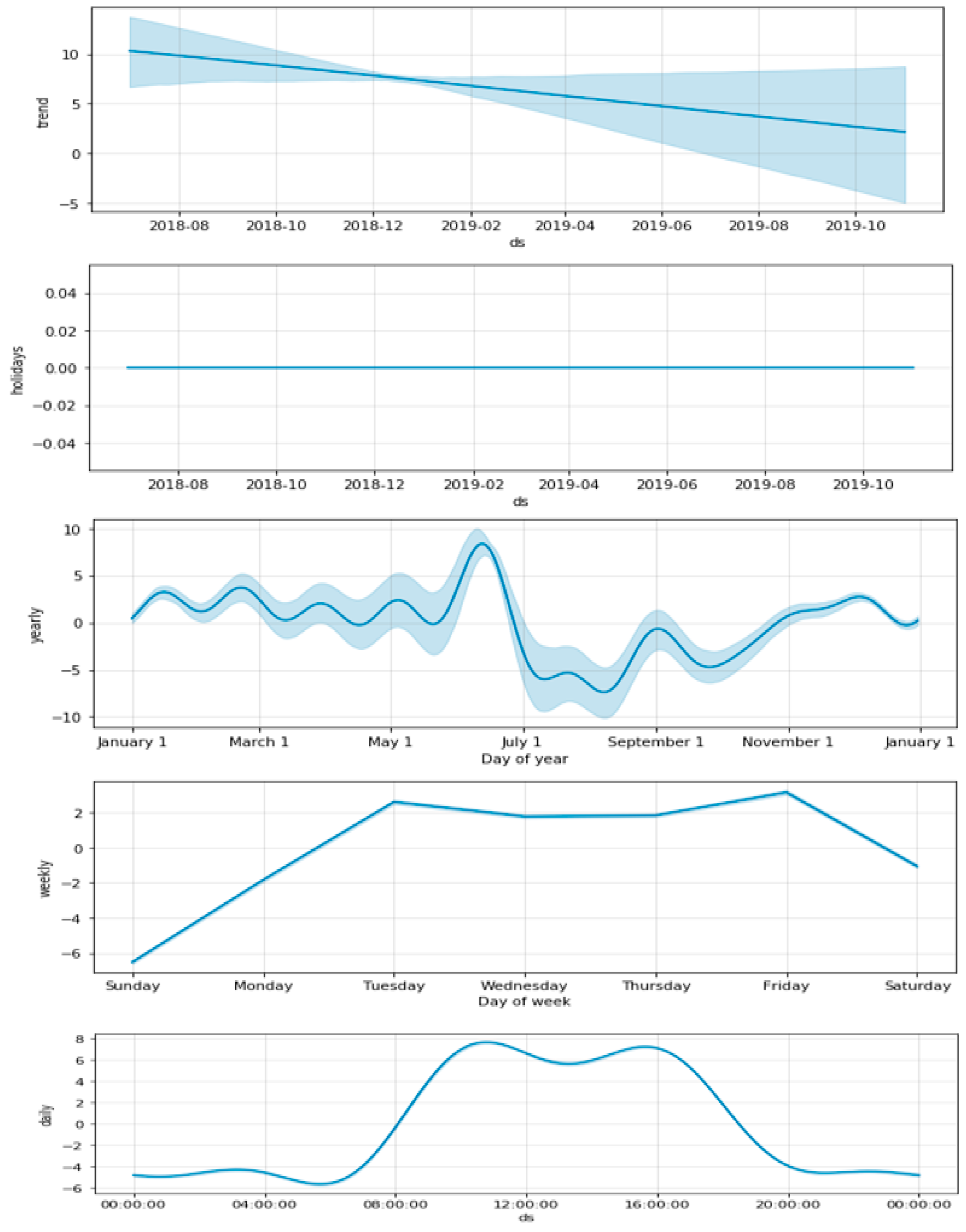
Figure 3. Trend, holidays, weekly, and daily prediction analysis of basic Prophet model. The blue line shows the trend the model fits from the test data and the light-blue shade shows the predicted trend.

Figure 3 displays the components (trend, holiday, weekly, and daily) of the fitted model. From Figure 3, we can observe that the trend and holidays exhibit relatively stable trends every month. The weekly component shows that electricity consumption occurs from Monday to Friday but not on weekends. The daily component shows that electricity consumption happens during working hours, from 8 a.m. to 8 p.m., and remains low during the rest of the day.

2.2. GRU Model

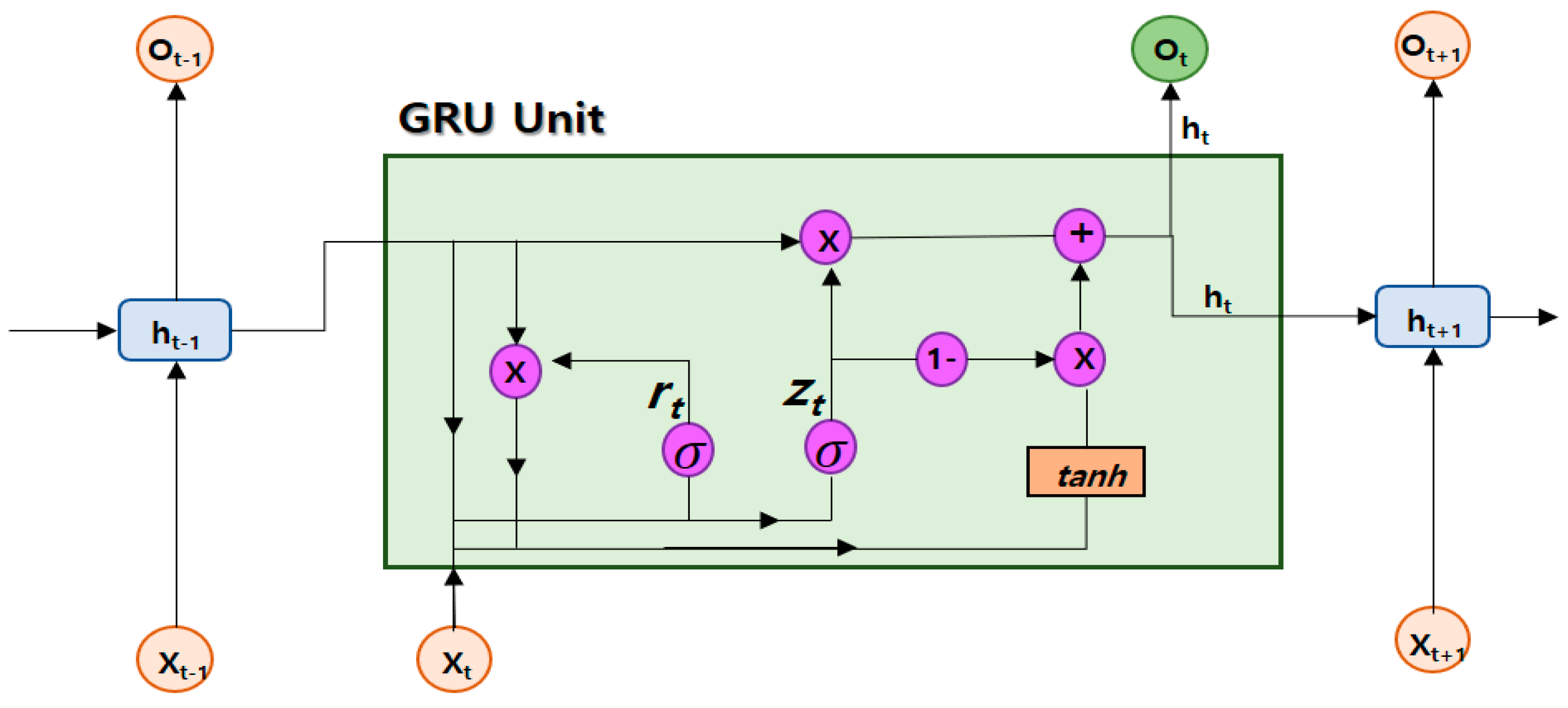
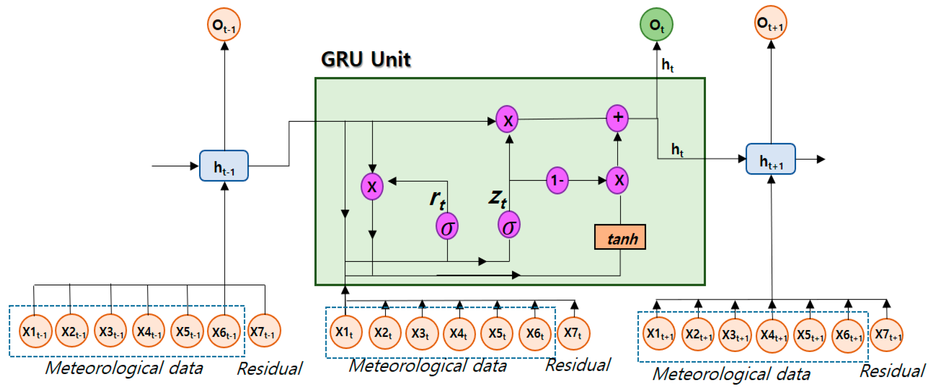
GRU, which stands for Gated Recurrent Unit, is a type of Recurrent Neural Network (RNN) used for processing sequence data [27]. It provides similar functionality to LSTM but has a simpler structure, as depicted in Figure 4. GRU addresses the vanishing gradient problem while learning long-term dependencies in sequence data and offers the advantage of reducing computational costs compared to LSTM.

Figure 4. GRU structure.

The components of GRU include the update gate, reset gate, and hidden state. Equation (2) represents the mathematical formulation of GRU. In Equation (2), $r_t$ denotes the reset gate, $z_t$ represents the update gate, $h_t$ is the hidden state, and $x_t$ signifies the current input. $W_z$ and $W_r$ are the weights for the update and reset gates, respectively.

$$\begin{array}{c}{z}_t=\sigma \left(W_z·\left[h_{t-1},x_t\right]\right)\hfill \\ r_t=\sigma \left(W_r·\left[h_{t-1},x_t\right]\right)\hfill \\ \widetilde{h_t}=tanh\left(W·\left[{r_t\times h}_{t-1},x_t\right]\right)\hfill \\ h_t=\left(1-z_t\right)\times h_{t-1}+z_t\times h_t\hfill \end{array}$$

(2)

GRU’s simplicity and effectiveness in handling long-term dependencies have made it a popular choice for various sequence data-processing tasks. It overcomes some limitations of traditional RNNs and is widely used in natural language processing, time-series analysis, and other fields that involve sequential data processing.

2.2.1. Update Gate

The update gate determines how much information to retain based on the current input and the previous hidden state. It is represented as a value between 0 and 1, where a value closer to 0 indicates that more past information will be forgotten and a value closer to 1 indicates that more information will be retained.

2.2.2. Reset Gate

The reset gate determines how much of the past information to forget based on the current input and the previous hidden state. It is represented as a value between 0 and 1, where a value closer to 0 indicates that more past information will be discarded and a value closer to 1 indicates that more past information will be preserved.

2.2.3. Hidden State

GRU computes a new hidden state based on the previous hidden state and the current input. It uses the update gate and the reset gate to control the combination of past and current information, resulting in the generation of a new hidden state.

3. Basic Prophet Model’s Problem and Solution

3.1. Basic Prophet Model’s Problem

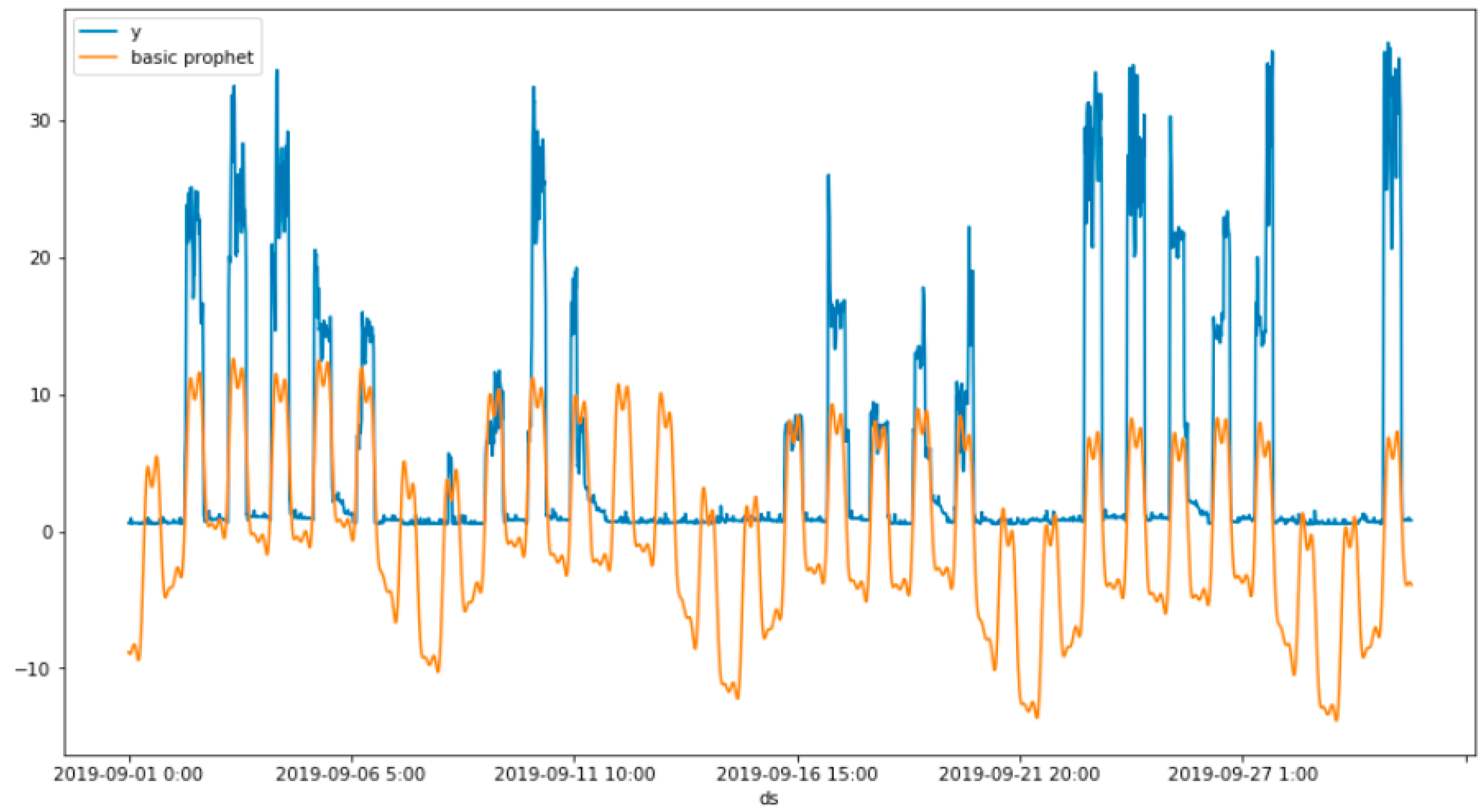
The advantage of the Prophet model is its ability to incorporate seasonality and events (holidays and public holidays) into the predictions. However, as shown in Figure 5, when applying the Prophet model from 1 September to 30 September 2019, there is a drawback where the observed values (y) during the 4-day thank-giving day (12 September to 15 September) are close to zero, but the Prophet model fails to accurately predict this.

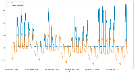
Figure 5. Performance comparison between observed value (y) and basic Prophet model (basic Prophet) from 1 July to 30 July 2019.

Therefore, when using the basic Prophet model, it is necessary to set parameters specifically for holiday information (duration, name) and consider the impact of holidays on electricity consumption before and after the holiday. Adjusting the flexibility of the trend and setting appropriate parameters for yearly seasonality are also necessary to better predict electricity consumption accurately.

3.2. Prophet Model’s Solution

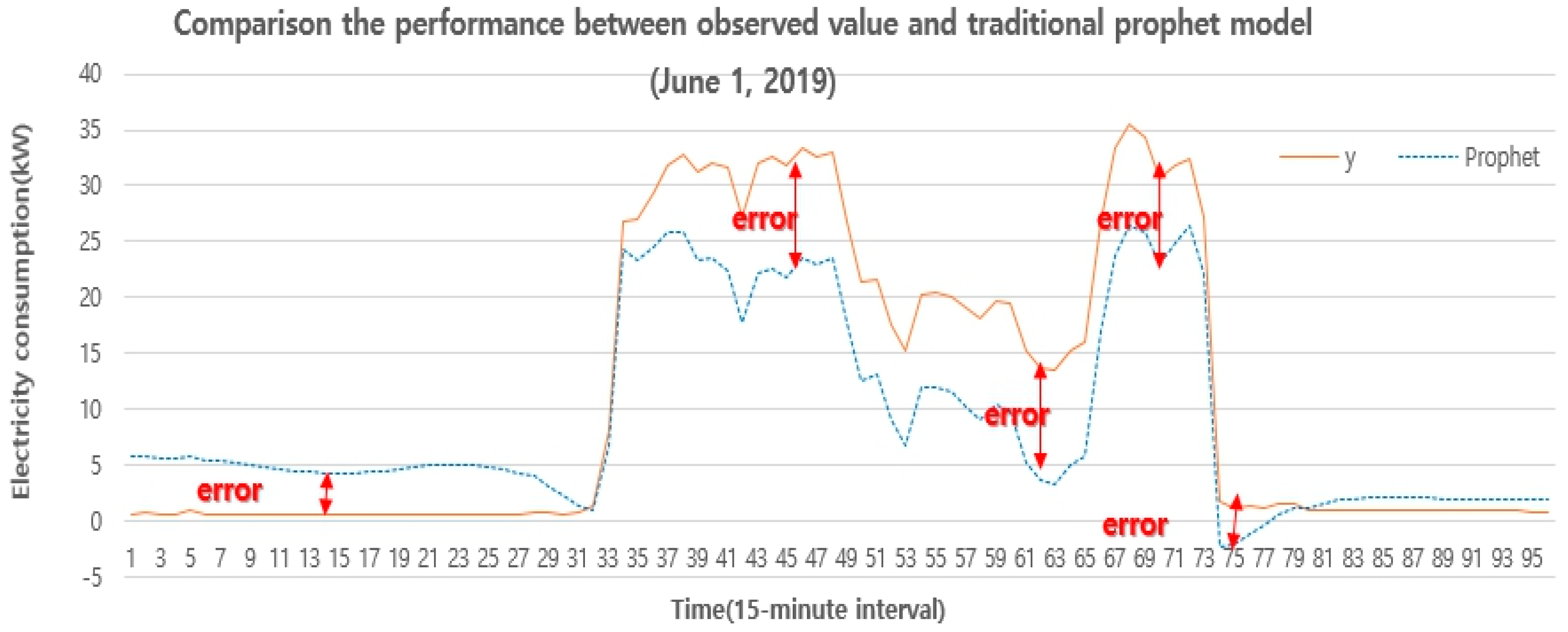
Figure 6 illustrates the discrepancies between the Prophet model (Prophet) and the observed values (y) for 1 July 2019, represented in 15 min intervals. In response to these discrepancies, the study incorporates GRU, a model well-suited for mid-term predictions, along with meteorological data known to influence building electricity consumption.

Figure 6. Performance comparison between the observed value (y) and the basic Prophet model’s value (Prophet) on 1 July 2019.

While applying GRU to the collected electricity consumption and meteorological data, the study openly acknowledges a limitation—the model’s inherent inability to handle information related to holidays and events. To surmount this constraint, the proposed approach merges Prophet, noted for its proficiency in managing holidays and events for long-term predictions, with GRU, tailored for short-term predictions. This strategic combination harnesses the unique strengths of each model to enhance the accuracy and overall performance of electricity consumption forecasting.

4. Proposed Methods

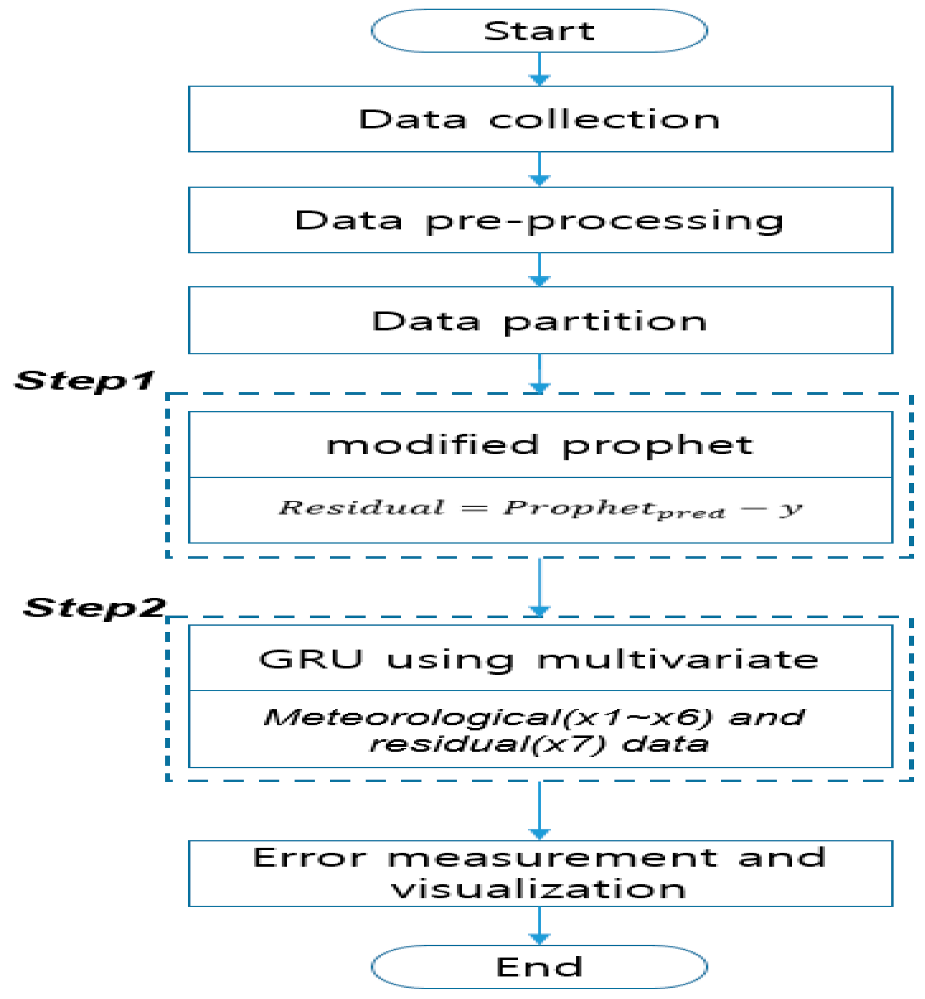
The flow chart of the proposed method in this study is shown in Figure 7. Section 4.1 explains how to collect data, Section 4.2 describes the pre-processing method for collected data, Section 4.3 describes how to divide data for learning and testing, Section 4.4 describes the proposed method using Prophet and GRU, and finally, the study concludes with error measurements and visualizations.

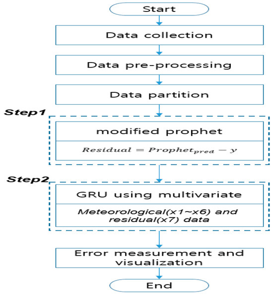
Figure 7. The flowchart of the proposed method.

4.1. Data Collection

In this study, the electricity consumption data used are collected from a company, B Corporation (machinery manufacturing), located in Naju, Jeollanam-do, Republic of Korea. The data spans from 1 July 2018 to 31 October 2019, with a time interval of 15 min.

Various factors, including Korean holidays (alternative holidays, election days, national holidays, etc.) are considered to enhance the accuracy of electricity consumption predictions. The workalendar package is utilized to generate the Korean holiday data. Additionally, meteorological data such as temperature, precipitation, wind speed, humidity, sunshine duration, and cloud cover are collected at hourly intervals from the Korea Meteorological Administration’s weather data portal (http://www.weather.go.kr, accessed on 10 November 2023).

4.2. Data Pre-Processing

The meteorological data are then resampled using linear interpolation to match the 15 min intervals of the electricity consumption data. To handle missing values in both power and meteorological data (temperature, precipitation, wind speed, humidity, sunshine duration, and cloud cover), they are filled with zeros. To reduce the impact of outliers for stable predictions and minimize the influence of nonlinear transformations, the RobustScaler method [28] is applied to normalize the data scale, as shown in Equation (3).

$$X_{scaled}=\frac{x-Q1\left(x\right)}{Q3\left(x\right)-Q1\left(x\right)}$$

(3)

In Equation (3), X_scaled is the scaled data, x is the original data, Q1(x) is the first quartile of the data, and Q3(x) is the third quartile of the data. By using RobustScaler, we ensure that the data are normalized while being less sensitive to the influence of outliers.

4.3. Data Partition for Training and Test Data

The training data span from 1 July 2018 to 30 June 2019, and the test data cover the period from 1 July 2019, to 31 October 2019. The data are divided into a 75% (365 days × 24 h × 15 min) portion for training and a 25% (123 days × 24 h × 15 min) portion for testing to conduct the experiments. Time-series data are sensitive to temporal order, so shuffling the data randomly can lead to the model making inaccurate predictions of future data. Therefore, in this study, we did not apply cross-validation.

4.4. Proposed Prophet Model

The experimental training data used in this study consist of electricity consumption data collected from 1 July 2018 to 30 June 2019. The modified Prophet model was simulated with components including trends, seasonality, holidays, flows, and others, as outlined in Table 1. Notably, the ‘df’ variable in the holiday parameters was adjusted to account for substitute holidays in this study. Both regular holidays and substitute holidays, such as election days and traditional holidays, within this time frame were taken into consideration to enhance the accuracy of electricity consumption predictions. The simulation results are shown in Figure 8 and Figure 9.

Table 1. Proposed Prophet model parameter setting.

Parameter Nature	Parameter Name	Value
Trend Parameters	growth	linear
	changepoints	None
	n_changepoints	25
	changepoint_range	0.8
	changepoint_prior_scale	0.01
Seasonality parameters	yearly_seasonality	10
	weekly_seasonality	False
	daily_seasonality	False
	seasonality_mode	multiplicative
	seasonality_prior_scale	10
Holidays parameters	holidays	df
	Holidays_prior_scale	0.25
Flow parameters	flow	flow
	flow_prior_scale	10
Other parameters	mcmc_samples	0
	interval_width	0.8

Figure 8. Error forecast of the proposed Prophet model. The black dots represent the historical input data, the blue line represents the predicted trend line after model fitting, and the light-blue area above and below the blue curve represents the confidence interval.

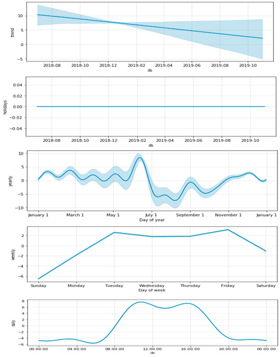
Figure 9. Trend, holidays, weekly, and daily prediction analysis of the proposed Prophet model. The blue line shows the trend the model fits from the test data and the light-blue shade shows the predicted trend.

In this study, the correlation coefficient was used as shown in Equation (4) to evaluate the accuracy of the long-term and short-term predictions [29].

$$r\left(X,Y\right)=\frac{1}{n}{\sum }_{i=1}^n\frac{(x_i-\overline{x})(y_i-\overline{y})}{{\sigma }_x{\sigma }_y}$$

(4)

In Equation (4), $\overline{x}$ and $\overline{y}$ represent the mean of X and Y, respectively, and ${\sigma }_x$ and ${\sigma }_y$ represent the standard deviation of X and Y, respectively, while n represents the number of data points.

For long-term predictions (1-year period) and short-term predictions (2 days), the correlation coefficients between the predicted electricity consumption and the observed consumption were found to be 0.67 and 0.87, respectively. This indicates that the modified Prophet model performs poorly for long-term electricity consumption predictions. However, the correlation coefficient of 0.87 for short-term predictions indicates that the model performs better than for long-term predictions. Therefore, the proposed Prophet model was used for short-term electricity consumption predictions.

4.5. Proposed GRU Model

To reduce the errors between the Prophet’s predictions and observed values, we propose incorporating GRU, as shown in Figure 10. Among various meteorological data that influence electricity consumption forecasting, the study adopted and utilized the six (temperature, precipitation, wind speed, humidity, sunshine duration, and cloud cover) most impactful variables for this study [30]. The input data consist of multiple variables, including meteorological data (temperature, precipitation, wind speed, humidity, sunshine duration, and cloud cover) and the residual (the difference between the predictions and observed values obtained from the Prophet model in the first step), totaling 7 variables.

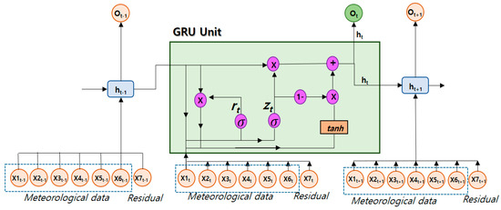
Figure 10. Structure of proposed GRU model.

In Figure 10, x1_t−1 to x6_t−1 represent the meteorological data from the previous time point (t − 1), i.e., temperature, precipitation, wind speed, humidity, sunshine duration, and cloud cover. x7_t−1 represents the residual. The traditional GRU prediction model typically targets the entire consumption data for electricity consumption predictions. However, in this study, we apply the residuals of the long-term trend (yearly and monthly) predictions to the GRU model, as shown in Equation (5), to predict electricity consumption and reduce error rates.

$$Residual={Prophet}_{pred}-y$$

(5)

In Equation (5), “Residual” denotes the residual, “Prophet_pred” represents the predictions obtained from the original Prophet model, and “y” is the observed consumption value. The GRU model’s training and validation data are derived from the same dataset. The input layer of the GRU model consists of 7 variables, which include 6 meteorological data variables (temperature, precipitation, wind speed, humidity, sunshine duration, cloud cover), and 1 residual variable. The hidden layer of the GRU model contains 7 nodes. Table 2 shows the training and testing options for simulating GRU. The initial learning rate is set to 0.005, and the maximum number of iterations is 500. The mean square error (MSE) for the loss function, ADAM [31] for the optimizer, and ReLU [32] for the activity function are employed during both training and testing.

Table 2. Training and testing option by GRU.

Parameter	GRU
Number of layers	7
Number of neurons	7
Number of epochs	500
Learning rate	0.005
Loss function	MSE
Optimization	ADAM
Weight initializer	1
Activation function	ReLU

5. Test Environment and Simulation Results

5.1. Test Environment and Software

To verify the Prophet model, GRU, and proposed methods, the experiments were performed on a workstation computer equipped with an Intel Xeon (R) W-2133 CPU, boasting a clock speed of 3.60 GHz CPU, and 3.60 GHz, and complemented by a generous 32 GB of RAM (Dell Precision 5820 Tower Workstation). The operating system was Windows 10 Pro for the workstations (64-bit). To conduct the experiments in this study, we employed the following approaches:

(1)

Utilizing Time-Series Prediction Libraries: For time-series forecasting, essential libraries such as scikit-learn [33], pandas [34], numpy [35], plotly [36], and others were employed. These libraries offer comprehensive tools for data manipulation, analysis, visualization, and modeling.

(2)

Implementing the Prophet Model: The implementation of the Prophet model was facilitated by employing the fbprophet library [37]. This dedicated library offers functionalities tailored for the Prophet forecasting framework, streamlining the process of working with seasonal and event-driven data.

(3)

GRU and Proposed Method Implementation: To experiment with GRU and the proposed hybrid method, we leveraged the Tensorflow [38] and Keras libraries [39]. These libraries are widely used in deep learning research and provide a platform for building, training, and evaluating neural network models like GRU.

By integrating these tools, we were able to effectively carry out the experiments outlined in the study, encompassing various aspects of time-series analysis, forecasting, and model evaluation.

5.2. Evaluation Metrics

To validate the proposed method in this study, error metrics including the correlation coefficient (CC), Root Mean Square (RMSE) [40], Root Mean Squared Scaled Error (RMSSE) [41], Mean Absolute Percentage Error (MAPE) [42], and Symmetric Mean Absolute Percentage Error (SMAPE) [43] were adopted. These metrics were utilized to assess the performance and accuracy of the proposed approach compared to other methods. Equations (6) and (9) are RMSE, MAPE, and SMAPE, respectively.

$$RMSE=\sqrt{\frac{1}{n}{\sum }_{i=1}^n{(y_i-\overline{y_i})}^2}$$

(6)

$$RMSSE=\sqrt{\frac{\frac{1}{n}{\sum }_{i=m+1}^{n+m}{(y_i-\overline{y_i})}^2}{\frac{1}{m-1}{\sum }_{i=2}^n{(y_i-y_{i-1})}^2}}$$

(7)

$$MAPE=\frac{100}{n}\times {\sum }_{i=1}^n\left|\frac{y_i-\overline{y_i}}{y_i}\right|$$

(8)

$$SMAPE=\frac{100}{n}\times {\sum }_{i=1}^n\frac{|y_i-\overline{y_i}|}{(\left|y_i\right|+|\overline{y_i}\left|\right)/2}$$

(9)

In Equations (6) and (9), $y_i$ is the actual value, $\overline{y_i}$ is the predicted value, m is the number of training data, and n is the number of test data.

5.3. Simulation Results

Table 3 provides the performance comparison of the Prophet, GRU, and proposed methods. The Prophet model was implemented using the approach proposed in step 1, while GRU involved seven simulations utilizing six meteorological datasets and one observed consumption dataset. The proposed method is a hybrid combining steps 1 and 2. The performance evaluation utilized several metrics, including the correlation coefficient (CC), RMSE, RMSSE, MAPE (%), and SMAPE (%). The correlation coefficient of the Prophet model decreased as the forecast period lengthened, whereas the correlation coefficients of GRU and the proposed method were consistently higher than that of the Prophet model regardless of the forecast period. The RMSE and RMSSE values of the Prophet model were 3–6 times higher than those of GRU and the proposed method, whereas the RMSE and RMSSE values of GRU and the proposed method were nearly similar. The MAPE of the Prophet model was 4–9 times higher than that of GRU and 9–23 times higher than that of the proposed method. Furthermore, the MAPE of GRU was more than twice as high as that of the proposed method. These results indicate that the proposed method outperformed both the Prophet and GRU models in terms of forecasting accuracy.

Table 3. Comparison of the performance of modified Prophet, GRU, and proposed method.

Term		Metrics	Prophet	GRU	Proposed
Short- term	2 days (1–2 July)	CC	0.88	0.97	0.97
		RMSE	7.77	2.97	2.97
		RMESE	49.50	18.92	18.92
		MAPE (%)	316.56	25.09	24.57
		SMAPE (%)	97.58	20.53	19.72
	7 days (1–7 August)	CC	0.51	0.97	0.98
		RMSE	6.08	1.44	1.41
		RMSSE	72.52	17.13	16.81
		MAPE (%)	526.62	48.07	27.32
		SMAPE (%)	123.01	59.07	30.09
Medium- term	15 days (1–15 Septermber)	CC	0.70	0.98	0.98
		RMSE	6.7	1.58	1.56
		RMSSE	115.88	27.50	27.24
		MAPE (%)	579.80	42.55	24.61
		SMAPE (%)	125.98	50.76	22.58
	30 days (1–30 October)	CC	0.67	0.97	0.98
		RMSE	7.48	2.25	2.22
		RMSSE	184.64	55.55	54.78
		MAPE (%)	348.06	37.66	34.37
		SMAPE (%)	103.92	42.48	33.28

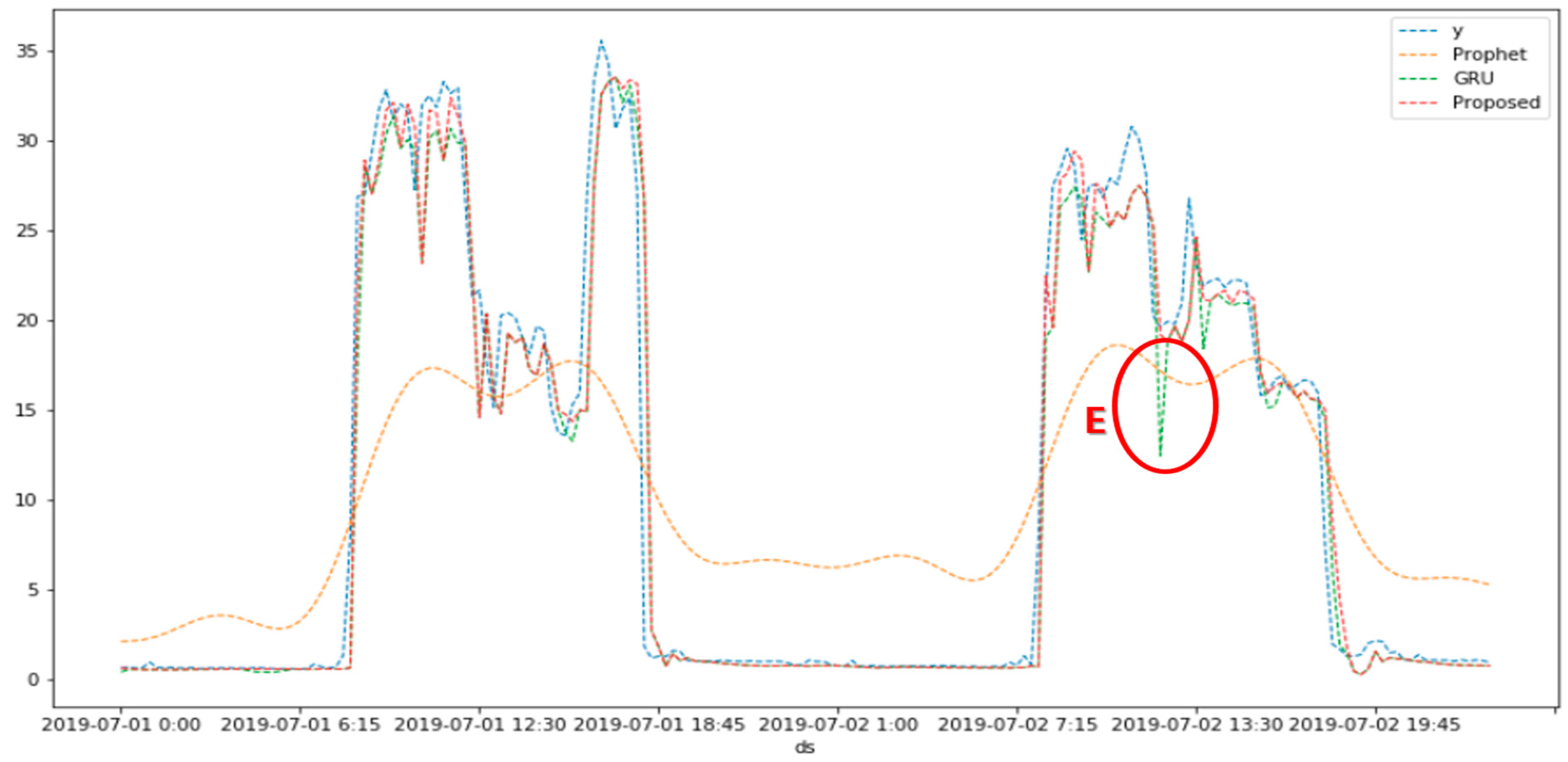
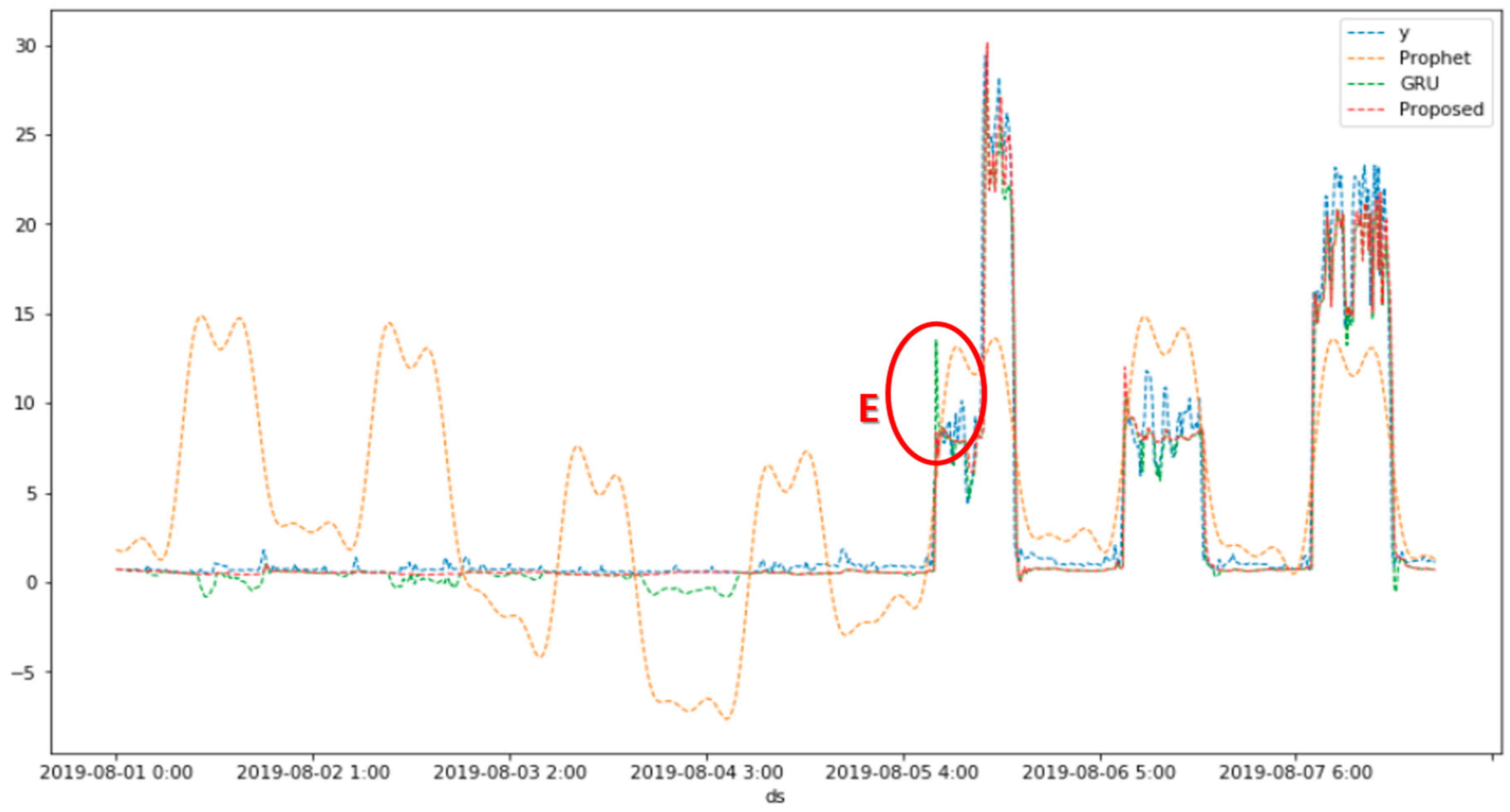
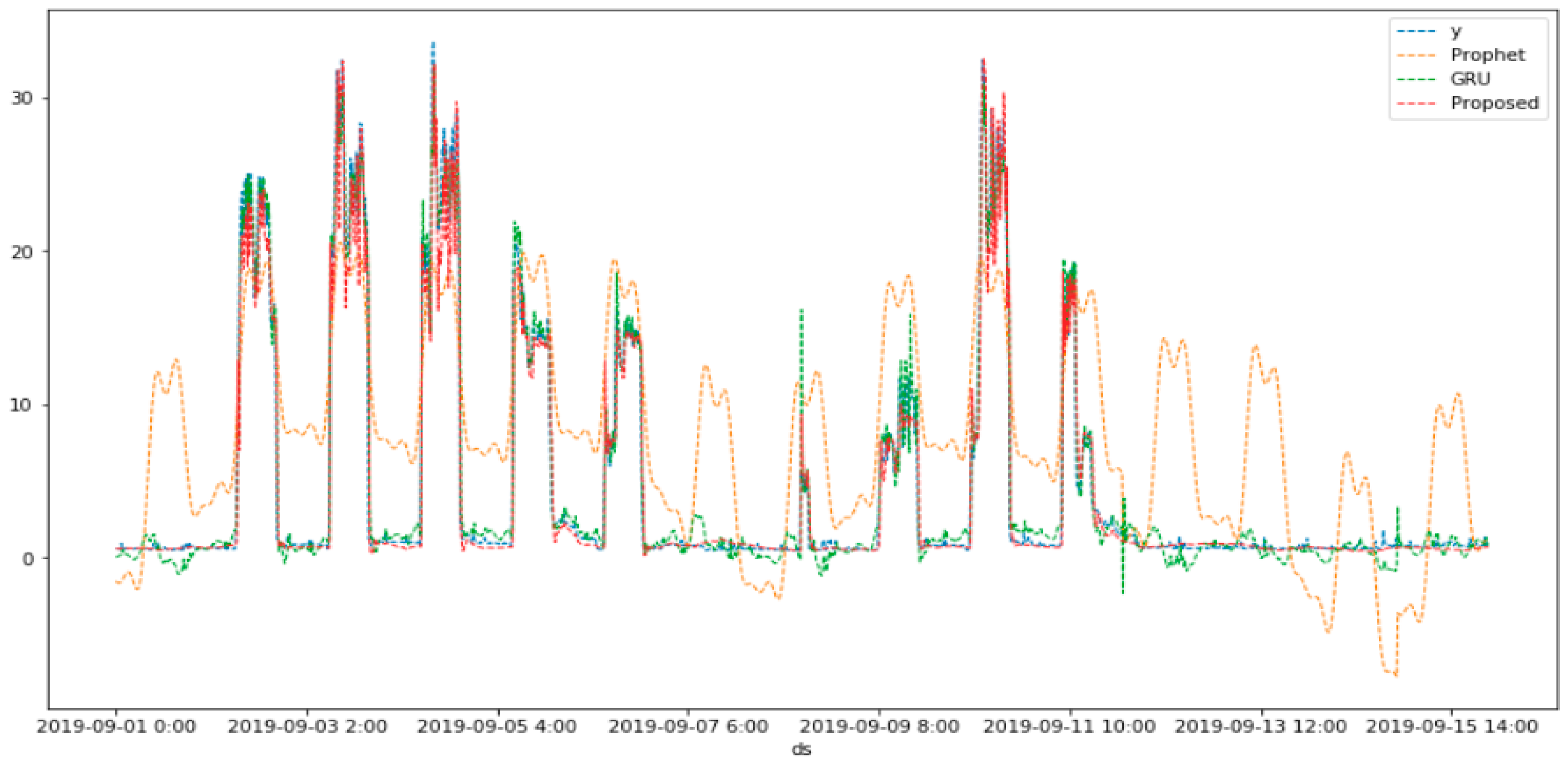
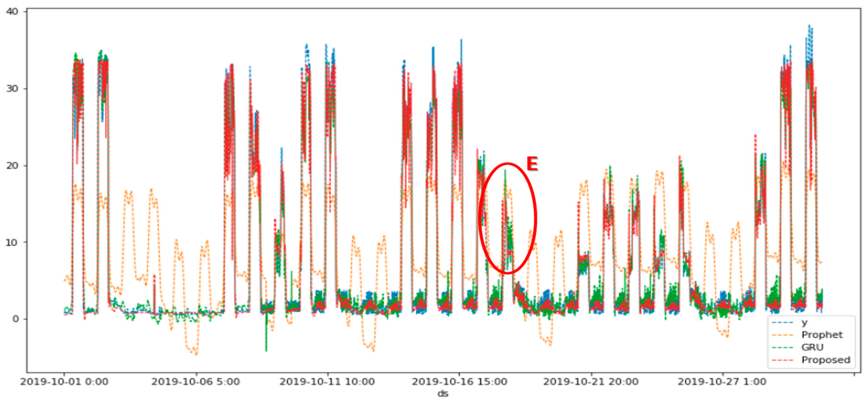
Figure 11, Figure 12, Figure 13 and Figure 14 illustrate the short-term electricity consumption forecasting comparisons for 2 days (1 July 2019 to 2 July 2019), 7 days (1 August 2019 to 7 August 2019), 15 days (1 September 2019 to 15 September 2019), and 30 days (1 October 2019 to 30 October 2019), respectively. In these figures, ‘y’ represents the observed consumption data measured during the specified periods, ‘Prophet’ denotes the modified Prophet model in Section 4.4, ‘GRU’ indicates the predicted values based on meteorological data and observed consumption data, and ‘Proposed’ signifies the predicted electricity consumption using the proposed method.

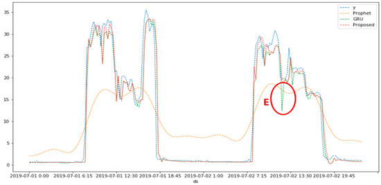
Figure 11. Comparison of graphic visualization performance between observed values (y) and other methods (modified Prophet, GRU using multivariate, and Proposed) from 1 July to 2 July 2019. The area “E” shows the largest prediction error in GRU.

Figure 12. Comparison of graphic visualization performance between observed values (y) and other methods (modified Prophet, GRU using multivariate, and Proposed) from 1 August to 7 August 2019. The area “E” shows the largest prediction error in GRU.

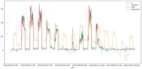
Figure 13. Comparison of graphic visualization performance between observed values (y) and other methods (modified Prophet, GRU using multivariate, and Proposed) from 1 September to 15 September 2019.

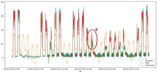
Figure 14. Comparison of graphic visualization performance between observed values (y) and other methods (modified Prophet, GRU using multivariate, and Proposed) from 1 October to 30 October 2019. The area “E” shows the largest prediction error in GRU.

In Figure 11, Figure 12, Figure 13 and Figure 14, the proposed method and ‘GRU’ closely resemble the observed consumption data (y), while ‘Prophet’ exhibits significantly high errors compared to the observed data (y). Notably, ‘GRU’ shows intermittent spikes in prediction errors, denoted in the “E” segment. Even during periods of minimal energy consumption, ‘GRU’ tends to generate numerous high predictions. This can be attributed to the model’s challenge in accurately predicting the occurrence of consecutive holidays or events, including substitute holidays, official holidays, and vacation periods. In contrast, the proposed method closely aligns with the observed consumption data (y), demonstrating superior accuracy in capturing these consumption patterns.

6. Conclusions

Electricity consumption forecasting is crucial in the electricity industry and energy system operations as it helps improve efficiency and stability. It provides valuable information to energy companies, power suppliers, network operators, and other stakeholders involved in energy management. This study proposes a short- and medium-term forecasting algorithm, combining the Prophet and GRU models, for predicting building electricity consumption over 2 days, 7 days, 15 days, and 30 days. The proposed method outperforms both the modified Prophet and GRU using multivariate.

Our proposed method offers a versatile and effective solution for optimizing energy management within Building Energy Management Systems, with the potential for substantial cost savings, improved energy source utilization, reduced carbon emissions, and enhanced operational efficiency, ultimately increasing the overall value of the building.

References

- International Renewable Energy Agency. Renewable Capacity Statistics; International Renewable Energy Agency: Masdar City, United Arab Emirates, 2020. [Google Scholar]
- Rethink Energy Site. Available online: https://rethinkresearch.biz/product/rethink-energy/ (accessed on 1 August 2023).
- Lv, L.; Luo, L.; Yang, Y. Distribution Line Load Predicting and Heavy Overload Warning Model Based on Prophet Method. Sustainability 2022, 14, 13697. [Google Scholar] [CrossRef]
- Grazioli, G.; Chlela, G.; Selosse, S.; Maïzi, N. The Multi-Facets of Increasing the Renewable Energy Integration in Power Systems. Energies 2022, 15, 6795. [Google Scholar] [CrossRef]
- Xue, B.; Keng, J. Dynamic Transverse Correction Method of Middle and Long Term Energy Forecasting Based on Statistic of Forecasting Errors. In Proceedings of the Conference on Power and Energy IPEC, Ho Chi Minh City, Vietnam, 12–14 December 2012; pp. 253–256. [Google Scholar]
- Enea, M. A review of machine learning algorithms used for load forecasting at micro-grid level. In Sinteza 2019-International Scientific Conference on Information Technology and Data Related Research; Singidunum University: Belgrade, Serbia, 2019; pp. 452–458. [Google Scholar]
- Brown, R.G. Smoothing Forecasting and Prediction of Discrete Time Series; Prentice-Hall: Englewood Cliffs, NJ, USA, 1963. [Google Scholar]
- Ohtsuka, Y.; Oga, T.; Kakamu, K. Forecasting electricity demand in Japan: A Bayesian spatial autoregressive ARMA approach. Comp. Stat. Data Anal. 2010, 54, 2721–2735. [Google Scholar] [CrossRef]
- Holt, C.E. Forecasting Seasonal and Trends by Exponentially Weighted Average; Carnegie Institute of Technology: Pittsburgh, PA, USA, 1957. [Google Scholar]
- Kalogirou, S.A.; Neocleous, C.C.; Schizas, C.C. Building Heating Load Estimation Using Artificial Neural Networks. In Proceedings of the 17th International Conference on Parallel Architectures and Compilation Techniques, San Francisco, CA, USA, 10–14 November 1997. [Google Scholar]
- Bagnasco, A.; Fresi, F.; Saviozzi, M.; Silvestro, F.; Vinci, A. Electrical consumption forecasting in hospital facilities: An application case. Energy Build. 2015, 103, 261–270. [Google Scholar] [CrossRef]
- Gers, F.; Schmidhuber, J.; Cummins, F. Learning to Forget: Continual Prediction with LSTM. In Neural Computation, Proceedings of the 9th International Conference on Artificial Neural Networks, Edinburgh, UK, 7–10 September 1999; MIT Press: Edinburgh, UK, 1999; pp. 850–855. [Google Scholar]
- Valenzuela, P.; Gorricho, J.; de la Iglesia. Automatic model and feature selection for time series forecasting: Achieving good performance and interpretability. Inf. Sci. 2018, 423, 157–174. [Google Scholar]
- Sanguansat, P.; Klomjit, N.; Hosseini, S.; Henao, N.; Amara, F. A comparative study of machine learning techniques for short-term load forecasting. In Proceedings of the 2021 IEEE International Conference on Communications, Control, and Computing Technologies for Smart Grids (SmartGridComm), Aachen, Germany, 25–28 October 2021. [Google Scholar]
- Junsuk, K.; Taejin, K. Application of Facebook’s Prophet Model for Forecasting Meteorological Data. J. Korean Soc. Hazard Mitig. 2021, 21, 53–58. [Google Scholar]
- Bashir, T.; Haoyong, C.; Tahir, M.F.; Liqiang, Z. Short-term electricity load forecasting using hybrid prophet-LSTM model optimized by BPNN. Energy Rep. 2022, 8, 1678–1686. [Google Scholar] [CrossRef]
- Serdar, A. A hybrid forecasting model using LSTM and Prophet for energy consumption with decomposition of time series data. PeerJ Comput. Sci. 2022, 8, e1001. [Google Scholar]
- Dinh, T.N.; Thirunavukkarasu, G.S.; Seyedmahmoudian, M.; Mekhilef, S.; Stojcevski, A. Energy Consumption Forecasting in Commercial Buildings during the COVID-19 Pandemic: A Multivariate Multilayered Long-Short Term Memory Time-Series Model with Knowledge Injection. Sustainability 2023, 15, 12951. [Google Scholar] [CrossRef]
- Li, P.; Zhang, J.S. A New Hybrid Method for China’s Energy Supply Security Forecasting Based on ARIMA and XGBoost. Energies 2018, 11, 1687. [Google Scholar] [CrossRef]
- Chen, Y.; Bhutta, M.S.; Abubakar, M.; Xiao, D.; Almasoudi, F.M.; Naeem, H.; Faheem, M. Evaluation of Machine Learning Models for Smart Grid Parameters: Performance Analysis of ARIMA and Bi-LSTM. Sustainability 2023, 15, 8555. [Google Scholar] [CrossRef]
- Zhang, G.P. Time Series Forecasting using a Hybrid ARIMA and neural network model. Neurocomputing 2003, 50, 159–175. [Google Scholar] [CrossRef]
- Pierre, A.A.; Akim, S.A.; Semenyo, A.K.; Babiga, B. Peak Electrical Energy Consumption Prediction by ARIMA, LSTM, GRU, ARIMA-LSTM and ARIMA-GRU Approaches. Energies 2023, 16, 4739. [Google Scholar] [CrossRef]
- Mancuso, P.; Piccialli, V.; Sudoso, A.M. A Machine Learning Approach for Forecasting Hierarchical Time Series. Expert Syst. Appl. 2021, 182, 115102. [Google Scholar] [CrossRef]
- Brégère, M.; Huard, M. Online Hierarchical Forecasting for Power Consumption Data. Int. J. Forecast. 2022, 38, 339–351. [Google Scholar] [CrossRef]
- Shi, X.; Chen, Z.; Wang, H.; Yeung, D.Y.; Wong, W.K.; Woo, W.C. Convolution LSTM Network: A Machine Learning Approach for Precipitation Nowcasting. Adv. Neural Inf. Process. Syst. 2015, 1, 802–810. [Google Scholar]
- Taylor, S.J.; Letham, B. Prophet: Forecasting at Scale. In Proceedings of the 22nd ACM SIGKDD International Conference on Knowledge Discovery and Data Mining, Halifax, NS, Canada, 13–17 August 2017; pp. 1389–1397. [Google Scholar]
- Cho, K.; Merriënboer, B.V.; Bahdanau, D.; Bengio, Y. On the properties of neural machine translation: Encoder-decoder approaches. arXiv 2014, arXiv:1409.1259. [Google Scholar]
- RobustScaler Documentation in Scikit-Learn. Available online: https://www.itl.nist.gov/div898/software/dataplot/refman2/auxillar/iqrange.htm (accessed on 26 August 2023).
- Sethna, J.P. Chapter 10: Correlations, response, and dissipation. In Statistical Mechanics: Entropy, Order Parameters, and Complexity; Oxford University Press: Oxford, UK, 2006; ISBN 978-0198566779. [Google Scholar]
- Son, N. Comparison of the Deep Learning Performance for Short-Term Power Load Forecasting. Sustainability 2021, 13, 12493. [Google Scholar] [CrossRef]
- Kingma, D.; Ba, J. Adam: A method for stochastic optimization. arXiv 2015, arXiv:1412.6980. [Google Scholar]
- Nair, V.; Hinton, G. Rectified linear units improve restricted Boltzmann machines. In Proceedings of the 27th International Conference on International Conference on Machine Learning, Haifa, Israel, 21–24 June 2010. [Google Scholar]
- Scikit-learn.org. Machine Learning in Python. Available online: https://scikit-learn.org/ (accessed on 26 August 2023).
- Pandas.org. Data Structure for Statistical Computing in Python. Available online: https://pandas.pydata.org/ (accessed on 26 August 2023).
- Numpy.org. Array Programming with NumPy. Available online: https://numpy.org/ (accessed on 26 August 2023).
- Plotly.org. Interactive Web-Based Data Visualization with R, Plot, and Shiny. Available online: https://plotly.org/ (accessed on 26 August 2023).
- Fbprophet.org. Forecasting at Scale. Available online: https://facebook.github.io/prophet/ (accessed on 26 August 2023).
- Tensorflow.org. Deep Learning Library Developed by Google. Available online: https://www.tensorflow.org/ (accessed on 26 August 2023).
- Keras.io. The Python Deep Learning Library. Available online: https://keras.io/ (accessed on 26 August 2023).
- Agresti, A. Categorical Data Analysis; John Wiley and Sons: New York, NY, USA, 1990. [Google Scholar]
- Hyndman, R.J.; Koehler, A.B. Another look at measures of forecast accuracy. Int. J. Forecast. 2006, 22, 679–688. [Google Scholar] [CrossRef]
- MAPE. Available online: https://en.wikipedia.org/wiki/Mean_absolute_percentage_error (accessed on 26 August 2023).
- SMAPE. Available online: https://en.wikipedia.org/wiki/Symmetric_mean_absolute_percentage_error (accessed on 26 August 2023).
Disclaimer/Publisher’s Note: The statements, opinions and data contained in all publications are solely those of the individual author(s) and contributor(s) and not of MDPI and/or the editor(s). MDPI and/or the editor(s) disclaim responsibility for any injury to people or property resulting from any ideas, methods, instructions or products referred to in the content. |
© 2023 by the authors. Licensee MDPI, Basel, Switzerland. This article is an open access article distributed under the terms and conditions of the Creative Commons Attribution (CC BY) license (https://creativecommons.org/licenses/by/4.0/).