Biodiversity and the Recreational Value of Green Infrastructure in England

Abstract

Green infrastructure refers to connected corridors of greenspaces within and beyond urban areas. It provides sustainable ecosystem goods and services for people and wildlife, enhancing their wellbeing and protecting them against climatic extremes. However, the exact contributing factors to the betterment of green infrastructure are not systematically examined at a national level. This study aims to identify what helps improve biodiversity and the recreational value of green infrastructure. The study uses hotspot analysis, ordinary least squares (OLS) regression and geographically weighted regression (GWR) to understand the spatial patterns of the relevant variables and outcomes. Findings suggest that high wildlife species richness was reported in Forestry Commission woodlands and country parks, whilst doorstep greens and village greens returned poor species richness. The recreational value of greenspace was affected the most by certain types of greenspace (e.g., woodlands) as well as the percentage of urban cover. They indicate that biodiversity is generally high in areas away from urban centres, while access to greenspace in an urban space brings us high recreational value. These results indicate that green infrastructure is a complex system that requires the right balance between different priorities and services.

1. Introduction

Green infrastructure (GI) is a comparatively modern idea, and its definition varies according to the discipline within which the term is applied. A common definition is “a spatial structure providing benefits from nature to people [which] aims to enhance nature’s ability to deliver multiple valuable ecosystem goods and services such as clean air or water” [1]. Another definition developed by the Green Infrastructure Work Group is “an interconnected network of waterways, wetlands, woodlands, wildlife habitats and other natural areas; greenways, parks and other conservation lands; working farms, ranches and forests; and wilderness and other open spaces that support native species, maintain natural ecological processes, sustain air and water resources and contribute to the health and quality of life for … communities and people” [2] (p. 1). The key is in the formation of a green corridor or a network of greenspace that meanders through the urban environment and connects rural and urban areas together. However, as a result of the difference in the scale of its components, GI is delivered at a variety of spatial scales from district to subregional levels [3], comprising individual street trees, private gardens, green roofs, rivers, verges and transport corridors, as well as larger infrastructure such as woodlands, parks, forests and wetlands [4]. The expected role of GI is to deliver a number of ecosystem services in both urban and rural settings [1]; namely, cultural services, regulation and maintenance services and provisioning services. Many of these services can be summarised as the provision of social and recreational benefits as well as benefits to wildlife [5].

The social and recreational benefits offered by GI are far-reaching, including the promotion of positive mental attitude and psychological health, increases in physical activity, improvement of human health and provision of areas for social interaction; whilst the environmental benefits comprise a reduction in day-time temperature [6], amelioration of the urban heat island effect [7], mitigation of surface water flooding [8], the removal of air pollution [9] and providing habitat connectivity [10]. Jerome et al. (2019) [11] suggest that out of the 14 factors that affect the quality of green infrastructure for people, the factors of most importance to defining quality were connectivity between GI, proximity to residences and that the habitats present form an ecological network. GI also has the potential to provide habitat and connectivity to wildlife. Cities in the United States of America have already seen an increase in wildlife sightings within them, as more cities have invested in green infrastructure to improve the local environment [12].

With the predicted change in climate becoming more apparent [13], a number of studies have investigated the ability of GI to alter the urban environment so that the effects of climate change can be managed or reduced. Predicted impacts of climate change include increases in temperature, rising sea levels, increases in extreme weather events and increases in the spread of diseases and pests [14,15]. The effects of climate change are likely to be more prevalent in urban areas [7]. However, climate change will also affect biodiversity with an increase in the intensity and frequency of droughts, storms and fires. Identifying which aspects of greenspaces can bring about the greatest benefit for people and wildlife is therefore paramount to help ameliorate the effects of climate change and, more generally, to increase the utility of GI.

Within England, GI is considered to consist primarily of large commissioned woods and countryside parks on the urban fringe, which are linked to parks, commons, gardens and doorstep greens in towns, and these greenspaces collectively form sustainable green corridors [4]. By networking the various greenspaces together, GI is seen as a mechanism for connecting urban to nature and providing recreational value to urban, suburban and rural communities alike whilst also reflecting responsibilities to the wider sustainable environment. It is also considered to contribute to wildlife species richness, supported by the diverse range of land uses and greenspace types [5]. However, despite that various government bodies, local authorities and local nature conservation organisations across England have launched agendas and roadmaps for utilizing GI for supporting urban life, the actual utility of GI, especially in terms of the recreational value it offers to the wider society, as well as the wildlife biodiversity it hosts, is yet to be studied systematically. Against this background, this study aims to clarify to what extent GI in England can offer value to society and wildlife and whether different types of greenspace offer different utility. Specifically, we investigate (1) whether wildlife species diversity is related to quality for people; (2) which variables have a significant effect on the wildlife species diversity of GI across England and how they are distributed; and (3) what variables contribute to the promotion of the social and recreational values of GI and how they are distributed across England. Findings from these pursuits are expected to fill some of the gaps we currently have in understanding the role and utility of GI for both society and wildlife. More generally, by addressing these research questions, we hope to measure whether GI indeed offers social and environmental values—measured in the forms of recreational value and wildlife species diversity—and, thereby, help the relevant stakeholders to reflect on the policies surrounding the provision of GI.

2. Literature Review

2.1. Impact of Green Infrastructure on Society

The impacts of greenspace on people are generally considered to be positive ones, many of which are measured with respect to their contribution towards the improvement of human health. For instance, many studies have reported how green infrastructure can directly impact human health, from reducing recovery time after surgery [16] to decreasing blood pressure [17,18]. While a majority of papers examined reported positive benefits of GI on life expectancy, Shanahan et al. (2015) [19] highlighted the presence of studies that found no association between mortality and greenspace coverage and one case that found higher mortality in proportionally greener cities. Maas et al. (2009) [20] also reported mixed results on how morbidity was related to the amount of greenspace present within a 1 km radius. There are even reports of “a small but significant association between LiDAR derived tree canopy extent and asthma and allergic sensitization” in African-American children in New York City [21] and certain tree species emitting biological volatile organic compounds and pollen as well as harbouring spore-producing mould [22]. These studies show that, in some circumstances, the addition of trees and the wider green infrastructure into residential areas could result in a negative effect on our wellbeing. These specific circumstances are often unravelled by investigating specific types of greenspace, tree species or other factors. In other words, while green infrastructure is considered to yield an overall positive value to people by offering visual, social and cultural benefits through its services, its detailed impact and any geographical variations may be teased out by investigating the difference between different greenspace types and any other attributes that distinguish them. Day and Smith (2016, 2017) [23,24] propose that the outdoor recreational value offered by green infrastructure can be measured by the estimated number of visits a greenspace might receive and the monetary equivalent of those visits. It would help to compare the difference in these recreational values across different parts of the UK to see what kind of underlying factors are affecting the outcome and what impact they might have on our wellbeing.

2.2. Impacts of Green Infrastructure on Wildlife

The literature available on the direct and indirect effects of GI on humans is wide-ranging but this is not the case with its impact on wildlife. GI has the potential to benefit wildlife by providing habitat connectivity in an increasingly urbanised world [25]. One of the most studied taxa in relation to GI usage is birds because they are relatively easy to survey, there are multiple survey methodologies and their life cycles are well understood [26]. Studies that assess the various aspects of greenspace that affect different species have yielded differing ranges of results with size, connectivity/isolation, the management regime and type of habitats present within the greenspaces all proving important [27,28,29]. For instance, Chamberlain et al. (2007) [30] reported that the site area, adjacency to gardens and presence of rough grass or waterbodies contributed to species richness among bird species in urban parks of London the most. The association between the size and species richness could be attributed to the large number of habitats in larger greenspaces, and other factors suggest that the size of the greenspace is not the most crucial factor. Negative associations were also recorded for the presence of buildings, roads and pavements across both the species groups and the seasons. Similarly, Zorzal et al. (2020) [29] reported that the taxonomic diversity of bird species recorded across six urban greenspaces in Brazil was positively associated with greenspace area but had an even stronger correlation with the heterogeneity of the habitats within each greenspace. Others examined the presence of red-listed bird species in Stockholm [27], bumble bee populations in the urban features of San Francisco [31], insect species richness in green roofs in Nova Scotia [32], amphibians in New Jersey [33] and bird species in the urban forest and managed parks of Ljubljana, Slovenia [34]. Most of these studies found that urbanicity or the embeddedness of the green infrastructure in urbanised areas seems to lower the level of biodiversity, irrespective of the size of each greenspace.

2.3. Use of Spatial Analysis in Determining Greenspace Quality

Many of the studies highlighted above do not account for the quality of the greenspace in their analyses, and they do not investigate the spatial patterns of these greenspaces either. The quality of GI can be evaluated using GIS and spatial modelling, where a set of spatial criteria may be combined with remote sensing data or other geographical representation and a scale of importance to determine regional environmental quality in order to direct restoration efforts [35]. For instance, a study looking at the effects on the spatial distribution of yellow perch in Lake Erie [36] utilised a geographically weighted regression model to visualise the effects of environmental variables on the wildlife species and aid in the management of fish stocks by improving the discrete areas at which the stocks are managed. Two of the management units reflected the discrete environmental variables, but the central management unit had environmental variables that acted on fish stocks at a finer scale.

Despite the intrinsically spatial nature of green infrastructure, its benefits and association with our values as well as biodiversity are still understudied from the spatial analytical perspective. By using a spatial analytical framework, this study aims to investigate the contributing factors that help improve the utility of green infrastructure and, thereby, gain insights into what aspects of green infrastructure contribute to better services.

3. Methodology and Data

3.1. Methods for Evaluating Green Infrastructure

Many of the studies identified above are based on small sample sizes or focus on one or two types of greenspace. To understand which types of greenspace offer true value for recreational, educational and environmental services, a wider range of greenspaces needs to be investigated.

This study investigates how the relationship between biodiversity and greenspaces varies across England and what kind of greenspace holds recreational value to us. England contains an estimated 27,000 public parks, and the provision of greenspace is a planning requirement with the National Planning Policy Framework [37]. It mandates new developments to provide safe and accessible areas with recreational, cultural and social facilities. These areas should support efforts to mitigate climate change effects and deliver wider benefits for nature. However, even though the NPPF encourages developments to include greenspace, the amount of greenspace in urban areas has dropped from 63% to 55% between 2001 and 2018 [38]. This highlights the need for urban greenspaces to have the highest possible quality to mitigate the loss of sites.

To evaluate the utility of green infrastructure, this study uses two sets of data, namely the biodiversity and the recreational values, as detailed below. The study starts with initial exploratory data analysis and mapping of their spatial patterns using scatterplots and Getis-Ord Gi*, respectively, to have a broad understanding of the relationship between the variables and the spatial patterns of the two dependent variables. The two factors will be then modelled with ordinary least squares (OLS) regression using prospective independent variables taken from the literature. The residual terms of the regression models will be checked for spatial dependency using local Moran’s I statistic and, if any systematic errors are present, we will proceed to carry out geographically weighted regression (GWR) modelling to identify the presence of spatial nonstationarity within the same subset of variables for both models. The coefficients of the variables in the GWR will be mapped, and a global Moran’s I test will be performed on the residuals to confirm the soundness of the model. These steps will ensure that we understand the geographical patterns of the different types of GI as well as the explanatory variables and how that reflects on the utility of different types of greenspace.

3.2. Wildlife Species and Biodiversity Data

This study aims to gain insights into the different values that each greenspace yields to our society and the habitats they offer to support biodiversity. The main focus of this study is on the diversity of wildlife species as in a select subset of animals and insect species that are hosted by the habitats of green infrastructure. The decision to exclude flora from this study is partly influenced by data availability but also based on the literature that reported the relationship between the richness of habitats within greenspace and wildlife diversity [25,26,27,28,29,30]. The National Biodiversity Network (NBN) provides access to aggregated biodiversity data from multiple recording schemes across England and Wales. The wildlife species data can be downloaded from the NBN gateway (nbnatlas.org) using the scientific name of each species. The maximum number of records the NBN gateway allows for downloading is 500,000 per wildlife species with a total of 10 million. To comply with this limit, the number of species included in the analysis was limited to those “of principal importance for the purpose of conserving biodiversity” (as specified in section 41 of the Natural Environment and Rural Communities (NERC) Act 2006) and is therefore considered to be recorded with care. The section 41 wildlife species list includes rare and threatened species across all classes. In this study, the following types of species were used: amphibians, birds, butterflies, mammals (including bats) and reptiles. Species groups such as beetles, moths and freshwater fish were excluded as they require specialist identification techniques and were recorded less frequently than other taxa. Other species highlighted as requiring further research were also excluded as they were likely under-recorded and may have skewed records across England.

The recordings are based on sighting reports and, while the number of specimens observed in each instance may vary, this study assumes each sighting as a single specimen and treats all records with unit weight. Some of the section 41 species are protected, and the sighting location is aggregated to 1 km resolution. To maintain uniformity of the data, all species records used in this study were renumerated to 1 km grid units.

Table 1. Number of records for each species group.

Species Group	Records
Amphibians	98,453
Bats	77,756
Birds	2,208,575
Butterflies	687,150
Mammal	430,380
Reptiles	136,514
Total	3,638,828

shows the total number of records for each species group found in and retrieved from the NBN database. Based on their spatial data, each record was assigned to the respective grid square, which enabled us to confirm the presence or absence of each species within each grid square and, thereby, derive the number of unique species in that grid square.

3.3. Greenspace Data and Recreational Values

The quality of greenspace assets can be quantified in a variety of forms, ranging from accessibility (proximity to urban areas) to the type of land cover as well as a composite index that represents a combination of various attributes of greenspace. The Outdoor Recreational Value (ORVal) tool, developed by the University of Exeter in collaboration with DEFRA, is an example of such a composite index tool used for describing the quality of greenspace. It gives an estimate of the quality of greenspaces across the UK for people using the estimated monetary value and the estimated visitor counts of each greenspace. The values are derived using the interactions among the habitats, legal designations of the site (including points of interest) and adjacency with other greenspaces.

Habitat areas in ORVal are determined based on a 25 m grid of the 2007 Land Cover Map (LCM) combined with Ordnance Survey Master Map data, the Priority Habitat Inventory dataset from Natural England [23] and Open Street Map data. The estimated greenspace visits are derived from the Monitor of Engagement with the Natural Environment (MENE) survey run by Natural England, which is a random sampling survey targeting adult residents of England taking a day trip for recreational purposes at a scale of 50,000 responses per year collected for six years. The underlying assumption is that someone visiting a single recreational greenspace would enjoy more welfare (or the recreational value) than they would when visiting other venues, and the amount of this welfare is estimated through an econometric model. Specifically, the estimated value of each greenspace is calculated through an opportunity cost model of recreational trip choice whilst taking into account the socioeconomic and environmental factors such as the socioeconomic and demographic profile of the visitors and time of the year as well as the attributes of a greenspace and qualities of alternative spaces in the vicinity. This estimate is derived as the ORVal score, which can be used as an indicator of a typical greenspace with the given features in that particular location. While these are estimated values, the ORVal II Modelling Report [24] indicates that improvements have been made through calibration with empirical data. Please refer to Day and Smith (2017, pp. 20–25) [24] for the details of the econometric model.

The GIS shapefile of the greenspace boundaries was also obtained through the ORVal portal. Polygons with missing data and private greenspaces (e.g., golf courses) were removed from the dataset, leaving 22,716 features.

Table 2. Types of publicly accessible greenspace across England.

Type of Greenspace	Count	Total Area (km2)	Avg. Area (km2)
Common	1283	12,649.60	9.86
Country Park	413	40,446.13	97.93
Doorstep Green	103	128.59	1.25
Forestry Commission Woods	193	54,132.82	280.48
Garden	331	1877.75	5.67
Millennium Green	81	176.26	2.18
Nature	2844	151,441.38	53.25
Park	9633	77,507.83	8.05
Village Green	669	1035.86	1.55
Woods	7166	152,363.77	21.26
Total	22,716	491,759.99	21.65

shows the number of records retrieved for each type of greenspace as well as the total area and the average area of each type of greenspace. Interestingly, parks, nature and common greenspace are the most frequent greenspace types but their average size, especially that of parks and common greenspace, is quite small compared to the average size of Forestry Commission woods and country parks, which, in turn, are less frequent. Other greenspace types such as doorstep greens, millennium greens, gardens and village greens are generally less frequent in their count and also small in their average size. While their presence is indispensable in the formation of green corridors across urban and rural areas, the compactness of their average size would likely restrict the number of unique wildlife species, which will be explored later.

4. Analysis

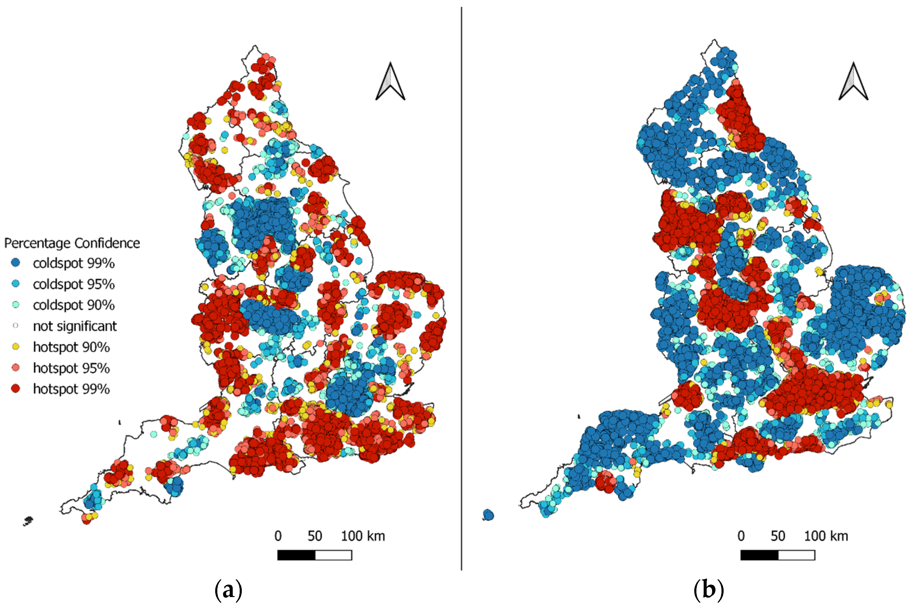
4.1. Species Richness and Recreational Value

To evaluate the benefit of green infrastructure from both the ecological and the social perspectives, this study examines the spatial distribution of the following indices:

(1)

The number of unique species as a representation of biodiversity;

(2)

The composite index of Outdoor Recreational Value estimated by ORVal.

The decision to use the number of unique species observed (species richness) as a proxy for biodiversity, instead of the total count of specimens observed or the number of habitats, was due to the other variables being proportional to the area of greenspace and, thereby, holding the risk of under-representing compact greenspaces that are rich in biodiversity. Due to data availability, only the species richness of fauna was considered but past review studies suggest that this would be permissible as a representation of biodiversity [39,40].

As both data showed log-normal distribution, they were log-transformed for the subsequent analyses. Figure 1 illustrates the spatial pattern of concentrations of log(species richness) (hereafter lsps) and log(recreational value) (hereafter lval), derived by applying Getis-Ord Gi* hotspot analysis to the z-scores of both variables.

Statistically significant clusters of high species richness (Figure 1a) were identified around well-known biodiverse landscapes such as the Mendips and the Somerset Levels and Moors, the New Forest and south coast, the southeast, Ainsdale and the Sefton coast, the Northumberland, Norfolk, and Suffolk coasts, the Chiltern Hills to Wicken Fen, the Wye Valley, the Herefordshire Hills, Bishops Castle and Thetford and Sherwood Forests. Coldspot clusters signifying a spatial continuum of low species richness were present in large cities including Greater London, Birmingham, Nottingham, Manchester and between Leeds and Sheffield. Interestingly, the recreational value shows the opposite tendency, where a majority of the statistically significant clusters of high lval (Figure 1b) were found in urbanised areas including Greater London and the surrounding areas up to Northampton, Manchester and Liverpool, Birmingham, Newcastle upon Tyne and the northeast coast and the south coast between Poole and Brighton.

4.2. Independent Variables for the Regression Modelling

To model the distribution of lsps and lval, the following variables were identified through the literature as possible contributing factors for species richness and recreational value: area, wood, natural grass, managed grass, parking, urban percentage, rivers and canals and the number of habitats. Figure 2 shows their scatterplots against lsps and lval. Whilst some of the combinations show positive correlations (e.g., log₁₀(woods) and log₁₀(number of unique wildlife species) return an adjusted R² value of 0.56, and the correlation between log₁₀(number of habitats) and log₁₀(number of unique wildlife species) interestingly remains low with adjusted R² = 0.10), most of them are only weakly positive even after transformation. The outputs of the scatterplots suggest that the analysis would be best achieved with nonparametric tests; however, due to the number of records involved, this may not be appropriate for this study as nonparametric tests may return inaccurate answers when used on large datasets [41,42].

To assess the spatial heterogeneity of each variable, local indicator of spatial autocorrelation (LISA) was performed using Moran’s I for each variable put towards the OLS regression (Figure 3). Area has very few but concentrated hot (high-high) spots in rural areas and even fewer cold (low-low) spots in urban areas. Other variables such as woodlands reflect the concentration around counties known for woods (e.g., Surrey) and coldspots in areas known for lower woodland cover (e.g., Suffolk and Somerset). Additionally, managed grassland habitat areas tend to be larger in urban areas, whilst natural grassland habitat areas are more prevalent in rural greenspaces. Parking is fairly sparse with some clusters in urban areas and coldspots in rural areas. Rivers and canals have large significant hotspots in the northwest and southwest with coldspots mainly concentrated in the south and southeast. The total number of habitats shows significant hotspots mainly in urban areas; however, as manmade habitats were included in the calculation of the number of habitats, there is perhaps a predisposition to urban areas with significant coldspots occurring in rural areas as there was with managed grasslands. The urban percentage clusters appear generally as expected.

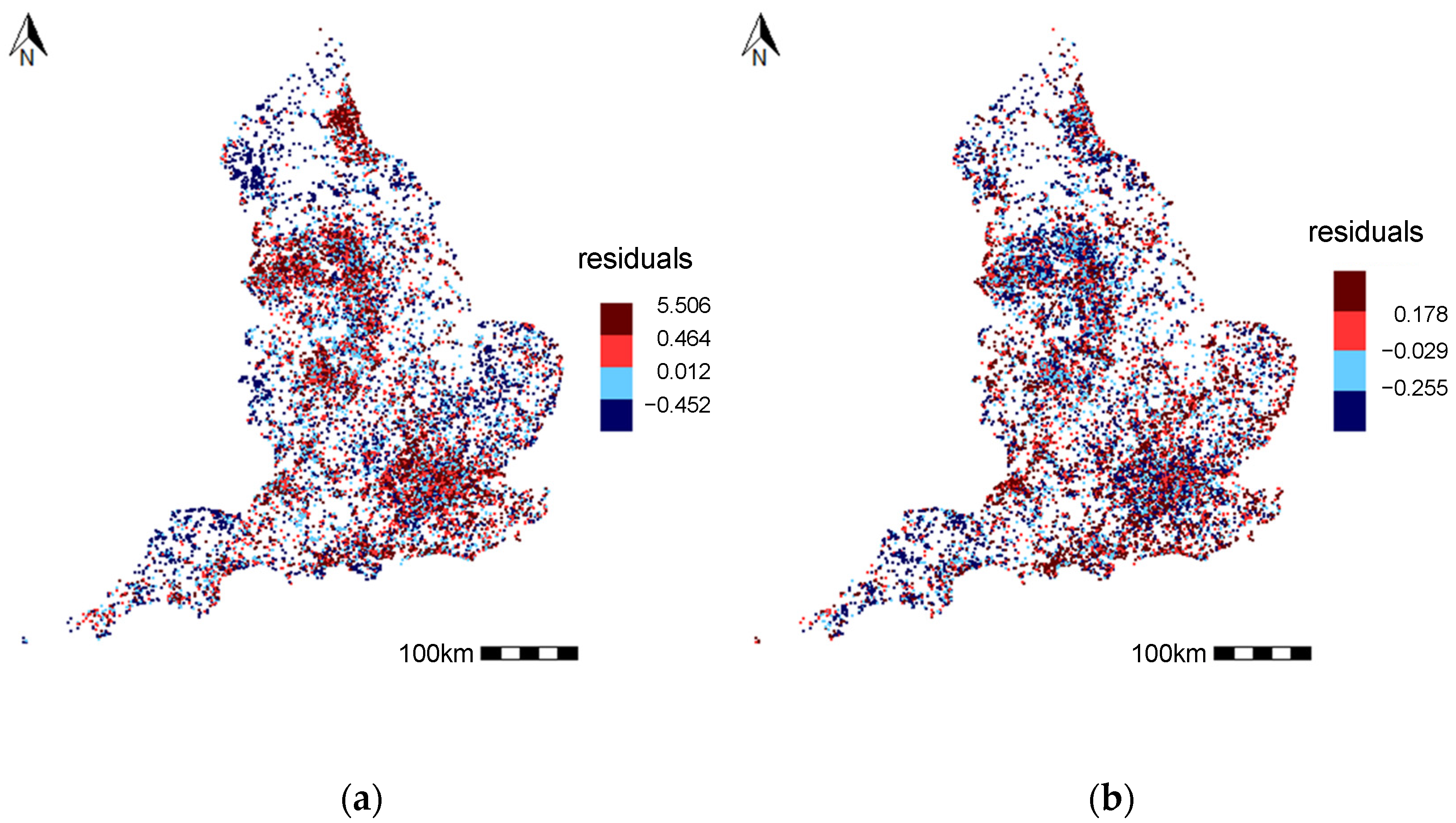
4.3. Ordinary Least Square (OLS) Regression Modelling

Using the variables described in the previous section, OLS regression models were computed (

Table 3. Results of OLS regression for lsps and lval, including the coefficients (*** denotes p-value < 0.001).

	lsps					lval
	Estimate	Std Error	t Value	Pr(>|t|)		Estimate	Std Error	t Value	Pr(>|t|)
X-Intercept	−0.281	0.015	−18.70	0.000	***	8.800	0.022	339.23	0.000	***
Area	0.001	0.000	22.14	0.000	***	0.000	0.000	−18.59	0.000	***
Woodland	0.516	0.003	150.83	0.000	***	0.272	0.005	54.19	0.000	***
Natural Grassland	0.301	0.007	42.75	0.000	***	0.056	0.010	5.40	0.000	***
Managed Grassland	0.194	0.006	32.45	0.000	***	0.079	0.009	9.00	0.000	***
Parking	0.407	0.021	19.71	0.000	***	1.140	0.030	37.55	0.000	***
Rivers/Canals	0.095	0.008	11.19	0.000	***	0.212	0.013	17.05	0.000	***
Number of Habitats	0.392	0.013	30.68	0.000	***	1.100	0.019	58.47	0.000	***
Urban Percentage	−0.204	0.015	−13.69	0.000	***	1.630	0.022	74.35	0.000	***

). Both lsps and lval models are sufficiently well specified, with adjusted R² values of R² = 0.76 and R² = 0.54, respectively.

Results from the lsps model (Table 3 left) show that there is a highly significant relationship for all variables with a low standard error (≤0.5162). The variables explained 76 % of the variance in species richness. The t-values indicate that the area of woodlands had the strongest positive relationship with species richness, whilst rivers and canals had the weakest relationship, if still positive. Urban percentage was shown to have a weak negative relationship.

Results from the lval model (Table 3 right) also indicate that all variables are highly significant with a low standard error (≤8.795). Whilst woods still had a strong positive relationship, urban percentage was shown to have more impact on the estimated value. Natural grassland habitat area had a weak positive relationship, and the overall site area had a moderate negative relationship.

Both models have small p-values and sufficiently large F-statistics to confirm their significance and reject the null hypothesis.

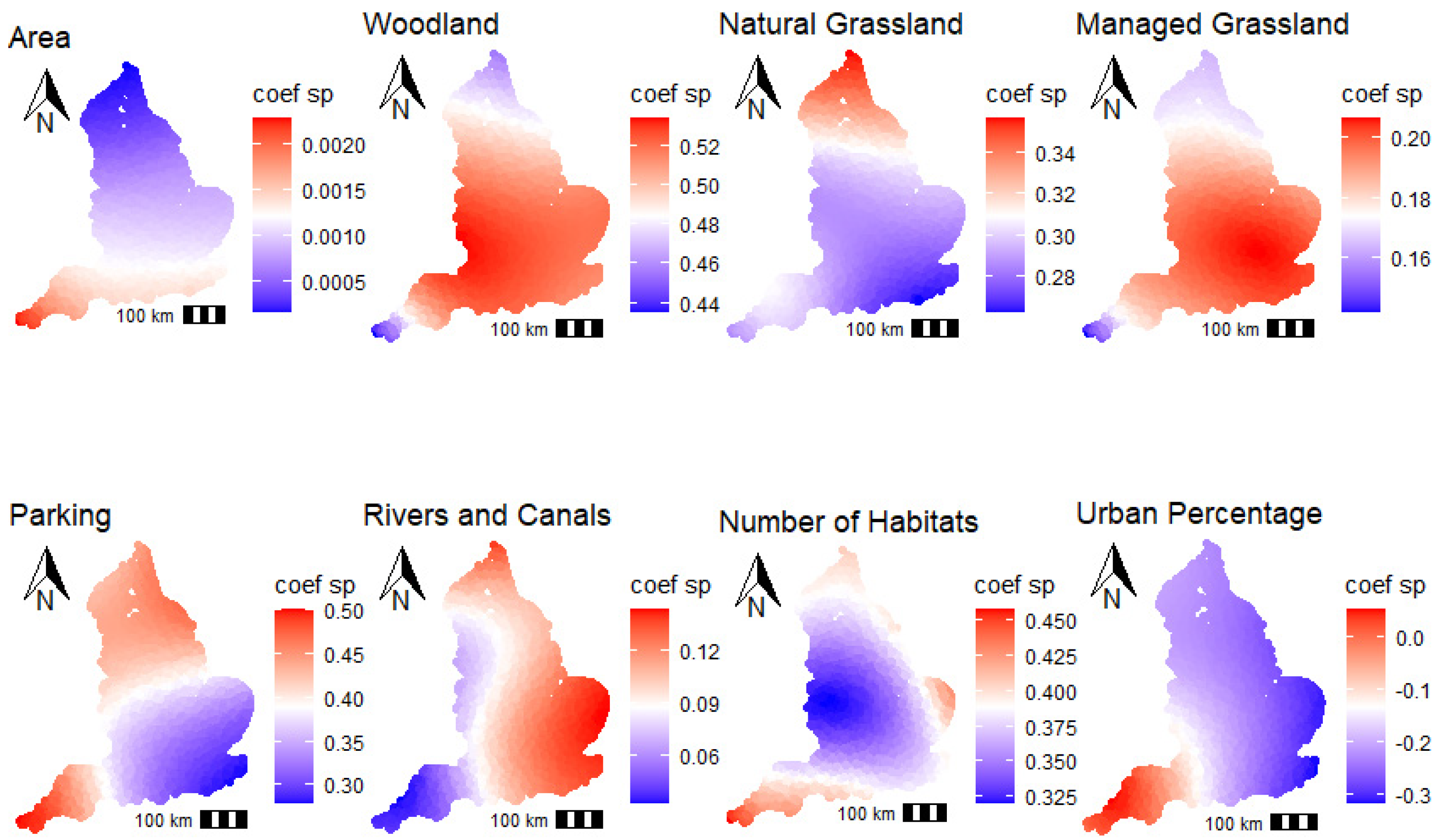
4.4. Geographically Weighted Regression (GWR) Modelling

The previous section showed that all variables, both dependent and independent, had some degrees of spatial bias, mostly affected by the urban–rural division, resulting in the formation of spatial clusters across England. To check whether these patterns match between the independent and the dependent variables and to alleviate the over-representations and under-representations arising from their spatial heterogeneity as needed, this study will proceed to use methods of spatial statistics.

Figure 4a,b show the distribution of the residual values from the OLS models for lsps and lval, respectively. Both figures illustrate the presence of spatial autocorrelation in the residual term of the regression models, suggesting that there are elements the models failed to explain.

To investigate this further and to reduce the amount of spatial autocorrelation in the residual term, both were analysed using a geographically weighted regression (GWR) model. The results of the GWR are shown in

Table 4. Correlation matrix from the GWR model for lsps (species richness).

	Area	Woodland	Natural Grassland	Managed Grassland	Parking	Rivers & Canals	Num. of Habitats	Urban Percentage
Area	1	0.55	−0.73	0.55	−0.58	0.06	0.26	0.44
Woodland	0.55	1	−0.81	0.90	−0.71	0.26	−0.46	0.02
Natural Grassland	−0.73	−0.81	1	−0.89	0.87	−0.45	0.23	0.16
Managed Grassland	0.55	0.90	−0.89	1	−0.90	0.60	−0.41	−0.27
Parking	−0.58	−0.71	0.87	−0.90	1	−0.78	0.07	0.39
Rivers & Canals	0.06	0.26	−0.45	0.60	−0.78	1	−0.01	−0.79
Num. of Habitats	0.26	−0.46	0.23	−0.41	0.07	−0.01	1	0.23
Urban Percentage	0.44	0.02	0.16	−0.27	0.39	−0.79	0.23	1

and

Table 5. Correlation matrix from the GWR model for lval (the recreational value).

	Area	Woodland	Natural Grassland	Managed Grassland	Parking	Rivers & Canals	Num. of Habitats	Urban Percentage
Area	1	0.59	−0.96	0.47	−0.38	−0.83	0.33	−0.05
Woodland	0.59	1	−0.64	0.33	−0.39	−0.46	0.23	−0.07
Natural Grassland	−0.96	−0.64	1	−0.45	0.37	0.76	−0.37	0.17
Managed Grassland	0.47	0.33	−0.45	1	−0.20	−0.46	−0.26	0.07
Parking	−0.38	−0.39	0.37	−0.20	1	0.25	−0.22	0.24
Rivers & Canals	−0.83	−0.46	0.76	−0.46	0.25	1	−0.41	−0.01
Num. of Habitats	0.33	0.23	−0.37	−0.26	−0.22	−0.41	1	−0.27
Urban Percentage	−0.05	−0.07	0.17	0.07	0.24	−0.01	−0.27	1

as coefficient matrixes, which are also plotted in Figure 5 and Figure 6, respectively. The global significance of the clustering of the GWR models was measured using global Moran’s I, and the lsps model returned a z-score of 0.91 (with a p-value of 0.86), whilst the lval model returned a z-score of 0.91 (with a p-value of 0.15). Both results suggest that any patterns remaining in the residuals are now random.

Figure 5 shows the coefficients for the variables in the lsps model. Most of them returned a narrow range of coefficients with the largest range being 0.37 for urban percentage. Greenspace area has more of an effect in the south of the country, whilst woodland generally has a higher effect on lsps in the centre of the country. The amount of natural grassland in a greenspace site appears to have more impact in the north of the country, whilst managed grassland is weighted more in the midlands and the east of the country. Parking has a greater effect in the southwest and north and less effect in the southeast. Greenspaces with rivers/canals in the southwest and west of the country have less effect on lsps than in the east, and the number of habitats within a greenspace appears to have more of an effect in the extreme southwest and Norfolk coast. Urban percentage has more of an impact on lsps in the east of the country and less of an impact in the southwest.

Plotting of the coefficients for recreational value (Figure 6) suggests that the greatest effect from the overall greenspace area on the estimated recreational value occurs in east Anglia and the southwest. The effects of woodland and rivers and canals on lval are greater in the east of the country and lower in the north and southwest. Natural grassland has a greater impact in the north, whilst managed grassland and parking have greater impacts in the north and southwest. The number of habitats has the most effect on recreational value in the northeast, whilst the effect of the percentage of urban cover is greatest in Norfolk with a reduced effect in the north of the country.

5. Discussion

Hotspot analysis for lsps (species richness) using Getis-Ord Gi* (Figure 1a) confirmed that the unique species counts showed strong spatial concentration in places known for species (e.g., New Forest and Jurassic Coast, Ainsdale NNR, Cambridge Fens and the coasts of Norfolk and Suffolk). The presence of hotspots primarily outside the urbanised area validates the use of the total unique species to determine species richness rather than using species abundance. The clusters of coldspots in the urbanised areas also confirm findings from previous studies in that species richness decreases with increasing urbanicity [31,32].

This means that, despite the fact that the green infrastructure movements advocate the provision of biodiversity across all manners of greenspace accessed and consumed by our society, the utility of such greenspace to wildlife varies between different areas and different types of greenspace, with those in urbanised areas holding less value as a biodiversity habitat. The modest contribution of area (total greenspace area) on species richness is somewhat surprising, but it also implies the presence of many factors affecting each species differently; e.g., area may have more impact on species with lower mobility but they also tend to be less conspicuous to visitors’ eyes. The relatively high effect of parking on species richness could be triggered by recording bias in that visitors may be more likely to record species presence in greenspaces made more accessible by parking.

In contrast, results from the hotspot analysis for lval (Figure 1b) broadly agree with the findings reported in previous studies in that green infrastructure in urbanised areas provides more direct benefits to people than it does in rural areas [43], meaning that areas such as London are expected to have a higher recreational value.

Gong et al. (2014) [44] noted that some socioeconomic groups prefer a more homogenous and easy-to-navigate landscape, which would explain the significance of managed grassland in the results. However, the large impact that woodlands have on lsps and lval may also be an artefact of the species data used. Bird records accounted for more than 60% of the records, and studies investigating the effects of landcover on bird diversity have shown a strong relationship between species richness and woodland cover [27,45]. The OLS regression models further confirmed the importance of the woodland area of a greenspace for predicting species richness. It supports the above notion that the heavy skew towards bird records within the original species data, together with the association between bird biodiversity and woodland area, may have overemphasised the relationship. Further analysis of the grouped species data would be necessary to identify if the same trends are found in other species groups such as mammals.

The strongest relationship for estimated recreational value was found to be the percentage of urban cover surrounding a greenspace. Assuming that the percentage of urban cover can be used as a proxy for accessibility, greenspaces with higher urbanicity are accessible to more people and will, therefore, generate higher recreational value than those at a greater distance. The higher cost of visiting greenspaces in remote areas (e.g., the Lake District) also results in a lower recreational value, and this is despite the fact that a large number of people may be willing to visit such areas [24]. This in turn may have exacerbated the effect of urban percentage even further.

Maps of the coefficients of the individual variables for the GWR model of lsps (Figure 5) do not necessarily reflect the original hot- and coldspot clusters present in their original spatial distribution (Figure 3). This suggests that the variance caused to species richness by these variables is unlikely to be geographical in origin or that the geographic variation cannot be discerned at this spatial scale. The exceptions are the GWR coefficients for managed grassland and natural grassland variables, both of which broadly follow the respective distributions.

Likewise, when comparing the results of the lval GWR to the variables plotted in Figure 6, none of the coefficients return the same geographical pattern as shown in the LISA analysis beyond the computational power available. However, global Moran’s I returned no significance on residuals for either of the GWR models, which suggests that the GWR models have accounted for the systematic error present in the residual terms of the OLS models, but it could also point to the presence of multicollinearity between variables, which would benefit from further investigation.

The effect of greenspace type on species richness appears to be bound up mainly in the average area of each greenspace type. For instance, both country parks and Forestry Commission woods tend to hold a large expanse of greenspace, which may explain their positive association with the number of unique species. Country parks have set criteria for designation including a minimum area of 10 ha or more, facilities and accessibility whilst being a predominantly seminatural landscape. As Forestry Commission woods are the largest supply of sustainably managed timber in the UK and commercial forestry operations require large amounts of land, Forestry Commission woodlands are on average the largest greenspace type within the analysis. An increase in area typically results in an increase in the number of habitat types and thus the available habitat niches, as well as a reduction in population isolation and disturbance [46], although species richness was not directly proportional to them.

6. Conclusions

This study investigated how and to what extent green infrastructure contributes to the provision of values as advocated in many policy documents. Specifically, we explored what recreational value it offers to the wider society and how much wildlife biodiversity it offers. The study found that areas of high wildlife species diversity tend to be found outside of urban areas, whilst areas of high estimated recreational value are usually located within urban areas. On the odd occasions where significant overlaps occurring between high species richness and high recreational value were identified in urban areas, they were found in larger greenspaces. Variables that affect both wildlife species richness and the estimated recreational value of greenspaces are the size of the greenspace, woodland cover, grassland cover (both managed and natural), rivers and canals, parking, number of habitats and percentage urban cover. Species richness was high in the types of greenspace that come in generally large sizes and in rural areas (e.g., country parks and Forestry Commission woods) and low in compact greenspaces in urban areas (e.g., village greens and doorstep greens).

Currently, much of the literature and policy documents embrace all manners of greenspaces as green infrastructure assets, but their utility differs greatly across different greenspace types, occasionally conflicting with one another, especially when it comes to their benefit to wildlife and to our society. Finding the balance between the two benefits requires wider planning decisions on where and how resources should be allocated to ensure the sustainability of both the wildlife and our society, and further investigation into this topic is expected to help establish the right balance between biodiversity and the recreational value offered by green infrastructure.

References

1. European Union. Green Infrastructure (GI)—Enhancing Europe’s Natural Capital. 2013. Available online: https://www.eea.europa.eu/policy-documents/green-infrastructure-gi-2014-enhancing (accessed on 1 December 2022).
2. Benedict, M.; MacMahon, E. Green infrastructure: Smart conservation for the 21st century. Renew. Resour. J. 2002, 20, 12–17. [Google Scholar]
3. Natural England. Natural England’s Green Infrastructure Guidance (NE176). 2009. Available online: http://publications.naturalengland.org.uk/file/94026 (accessed on 1 December 2022).
4. UK Green Building Council. Demystifying Green Infrastructure. 2015. Available online: https://ukgbc.s3.eu-west-2.amazonaws.com/wp-content/uploads/2017/09/05153004/Demystifying-Green-Infrastructure-report-FINAL.pdf (accessed on 1 December 2022).
5. Millennium Ecosystem Assessment. Ecosystems and Human Well-Being: Synthesis; Island Press: Washington, DC, USA, 2005. [Google Scholar]
6. Georgi, N.J.; Zafiriadis, K. The impact of park trees on microclimate in urban areas. Urban Ecosyst. 2006, 9, 195–209. [Google Scholar] [CrossRef]
7. Emilsson, T.; Sang, Å.O. Impacts of climate change on urban areas and nature-based solutions for adaptation. In Nature-Based Solutions to Climate Change Adaptation in Urban Areas: Linkages between Science, Policy and Practice; Kabisch, N., Korn, H., Stadler, J., Bonn, A., Eds.; Springer International Publishing: Cham, Switzerland, 2017; pp. 15–27. [Google Scholar]
8. Ellis, J.B.; Lundy, L.; Revitt, D.M. An impact assessment methodology for urban surface runoff quality following best practice treatment. Sci. Total Environ. 2012, 416, 172–179. [Google Scholar] [CrossRef] [PubMed]
9. Bottalico, F.; Chirici, G.; Giannetti, F.; de Marco, A.; Nocentini, S.; Paoletti, E.; Salbitano, F.; Sanesi, G.; Serenelli, C.; Travaglini, D. Air pollution removal by green infrastructures and urban forests in the City of Florence. Agric. Agric. Sci. Proc. 2016, 8, 243–251. [Google Scholar] [CrossRef]
10. Liquete, C.; Kleeschulte, S.; Dige, G.; Maes, J.; Grizzetti, B.; Olah, B.; Zulian, G. Mapping green infrastructure based on ecosystem services and ecological networks: A Pan-European case study. Environ. Sci. Policy 2015, 54, 268–280. [Google Scholar] [CrossRef]
11. Jerome, G.; Sinnett, D.; Burgess, S.; Calvert, T.; Mortlock, R. A framework for assessing the quality of green infrastructure in the built environment in the UK. Urban For. Urban Gree. 2019, 40, 174–182. [Google Scholar] [CrossRef]
12. Hunold, C. Green infrastructure and urban wildlife: Toward a politics of sight. Humanimalia 2019, 11, 89–109. [Google Scholar] [CrossRef]
13. Arntz, W.; Strobel, A.; Moreira, E.; Mark, F.; Knust, R.; Jacob, U.; Brey, T.; Barrera-Oro, E.; Mintenbeck, K. Impact of climate change on fishes in complex Antarctic ecosystems. Adv. Ecol. Res. 2012, 46, 351–426. [Google Scholar]
14. Forzieri, G.; Feyen, L.; Russo, S.; Vousdoukas, M.; Alfieri, L.; Outten, S.; Migliavacca, M.; Bianchi, A.; Rojas, R.; Cid, A. Multi-hazard assessment in Europe under climate change. Clim. Chang. 2016, 137, 105–119. [Google Scholar] [CrossRef]
15. IPCC Secretariat. Scientific Review of the Impact of Climate Change on Plant Pests. 2021. Available online: https://www.fao.org/3/cb4769en/cb4769en.pdf (accessed on 1 December 2022).
16. Ulrich, R.S. View through a window may influence recovery from surgery. Science 1984, 224, 420–421. [Google Scholar] [CrossRef]
17. Thompson, C.W.; Roe, J.; Aspinall, P.; Mitchell, R.; Clow, A.; Miller, D. More green space is linked to less stress in deprived communities: Evidence from salivary cortisol patterns. Landsc. Urban Plan. 2012, 105, 221–229. [Google Scholar] [CrossRef]
18. Grazuleviciene, R.; Vencloviene, J.; Kubilius, R.; Grizas, V.; Dedele, A.; Grazulevicius, T.; Ceponiene, I.; Tamuleviciute-Prasciene, E.; Nieuwenhuijsen, M.J.; Jones, M.; et al. The effect of park and urban environments on coronary artery disease patients: A randomized trial. BioMed. Res. Int. 2015, 2015, 403012. [Google Scholar] [CrossRef] [PubMed] [Green Version]
19. Shanahan, D.F.; Lin, B.B.; Bush, R.; Gaston, K.J.; Dean, J.H.; Barber, E.; Fuller, R. Toward improved public health outcomes from urban nature. Am. J. Public Health 2015, 105, 470–477. [Google Scholar] [CrossRef]
20. Maas, J.; Verheij, R.; de Vries, S.; Spreeuwenberg, P.; Schellevis, F.; Groenewegen, P. Morbidity is related to a green living environment. J. Epidemiol. Community Health 2009, 63, 967–973. [Google Scholar] [CrossRef] [PubMed]
21. Hartig, T.; Mitchell, R.; de Vries, S.; Frumkin, H. Nature and health. Annu. Rev. Public Health 2014, 35, 207–228. [Google Scholar] [CrossRef]
22. Tomalak, M.; Rossi, E.; Ferrini, F.; Moro, P. Negative aspects and hazardous effects of forest environment on human health. In Forests, Trees and Human Health; Nilsson, K., Sangster, M., Gallis, C., Hartig, T., de Vries, S., Seeland, K., Schipperijn, J., Eds.; Springer: Dordrecht, The Netherlands, 2010; Chapter 4; pp. 77–126. [Google Scholar]
23. Day, B.; Smith, G. Outdoor Recreational Valuation (ORVal) Data Set Construction, University of Exeter. 2016. Available online: https://www.leep.exeter.ac.uk/orval/pdf-reports/orval_data_reportOLD.pdf (accessed on 1 December 2022).
24. Day, B.; Smith, G. The ORVal Recreation Demand Model: Extension Project, University of Exeter. 2017. Available online: https://www.leep.exeter.ac.uk/orval/pdf-reports/ORValII_Modelling_Report.pdf (accessed on 1 December 2022).
25. Zhang, S.; Ramírez, F. Assessing and mapping ecosystem services to support urban green infrastructure: The case of Barcelona, Spain. Cities 2019, 92, 59–70. [Google Scholar] [CrossRef]
26. Leveau, L.M.; Isla, F.I. Predicting bird species presence in urban areas with NDVI: An assessment within and between cities. Urban For. Urban Gree. 2021, 63, 127199. [Google Scholar] [CrossRef]
27. Mörtberg, U.; Wallentinus, H.G. Red-listed forest bird species in an urban environment—Assessment of green space corridors. Landsc. Urban Plan. 2000, 50, 215–226. [Google Scholar] [CrossRef]
28. Holtmann, L.; Philipp, K.; Becke, C.; Fartmann, T. Effects of habitat and landscape quality on amphibian assemblages of urban stormwater ponds. Urban Ecosyst. 2017, 20, 1249–1259. [Google Scholar] [CrossRef]
29. Zorzal, R.; Diniz, P.; Oliveira, R.; Duca, C. Drivers of avian diversity in urban greenspaces in the Atlantic Forest. Urban For. Urban Gree. 2020, 59, 126908. [Google Scholar] [CrossRef]
30. Chamberlain, D.E.; Gough, S.; Vaughan, H.; Vickery, J.A.; Appleton, G.F. Determinants of bird species richness in public green spaces. Bird Study 2007, 54, 87–97. [Google Scholar] [CrossRef]
31. McFrederick, Q.S.; LeBuhn, G. Are urban parks refuges for bumble bees Bombus spp. (Hymenoptera: Apidae)? Biol. Conserv. 2006, 129, 372–382. [Google Scholar] [CrossRef]
32. MacIvor, J.S.; Ksiazek-Mikenas, K. Invertebrates on Green Roofs. In Green Roof Ecosystems; Sutton, R.K., Ed.; Springer International Publishing: Cham, Switzerland, 2015; pp. 333–355. [Google Scholar]
33. Mccarthy, K.; Lathrop, R. Stormwater basins of the New Jersey coastal plain: Subsidies or sinks for frogs and toads? Urban Ecosyst. 2011, 14, 395–413. [Google Scholar] [CrossRef]
34. de Groot, M.; Flajšman, K.; Mihelič, T.; Vilhar, U.; Simončič, P.; Verlič, A. Green space area and type affect bird communities in a South-eastern European city. Urban For. Urban Gree. 2021, 63, 127212. [Google Scholar] [CrossRef]
35. Rahman, M.R.; Shi, Z.H.; Chongfa, C. Assessing regional environmental quality by integrated use of remote sensing, GIS, and spatial multi-criteria evaluation for prioritization of environmental restoration. Environ. Monit. Assess. 2014, 186, 6993–7009. [Google Scholar] [CrossRef]
36. Liu, C.; Liu, J.; Jiao, Y.; Tang, Y.; Reid, K. Exploring spatial nonstationary environmental effects on Yellow Perch distribution in Lake Erie. PeerJ 2019, 7, e7350. [Google Scholar] [CrossRef] [PubMed]
37. Ministry of Housing, Communities & Local Government. The National Planning Policy Framework. 2021. Available online: https://www.gov.uk/government/publications/national-planning-policy-framework--2 (accessed on 1 December 2022).
38. Public Health England. Improving Access to Greenspace: A New Review for 2020. 2020. Available online: https://assets.publishing.service.gov.uk/government/uploads/system/uploads/attachment_data/file/904439/Improving_access_to_greenspace_2020_review.pdf (accessed on 1 December 2022).
39. Williams, P.H.; Humphries, C.J.; Vane-Wright, R.I. Measuring biodiversity: Taxonomic relatedness for conservation priorities. Aust. Syst. Bot. 1991, 4, 665–679. [Google Scholar] [CrossRef]
40. Löki, V.; Deák, B.; Lukács, A.B.; Molnár, V.A. Biodiversity potential of burial places—A review on the flora and fauna of cemeteries and churchyards. Glob. Ecol. Conserv. 2019, 18, e00614. [Google Scholar] [CrossRef]
41. Skovlund, E.; Fenstad, G. Should we always choose a nonparametric test when comparing two apparently nonnormal distributions? J. Clin. Epidemiol. 2001, 54, 86–92. [Google Scholar] [CrossRef] [PubMed]
42. Fagerland, M.W. T-tests, non-parametric tests, and large studies—A paradox of statistical practice? BMC Med. Res. Methodol. 2012, 12, 78. [Google Scholar] [CrossRef] [PubMed]
43. de Jalón, S.G.; Chiabai, A.; Quiroga, S.; Suárez, C.; Ščasný, M.; Máca, V.; Zvěřinová, I.; Marques, S.; Craveiro, D.; Taylor, T. The influence of urban greenspaces on people’s physical activity: A population-based study in Spain. Landsc. Urban Plan. 2021, 215, 104229. [Google Scholar] [CrossRef]
44. Gong, Y.; Gallacher, J.; Palmer, S.; Fone, D. Neighbourhood green space, physical function and participation in physical activities among elderly men: The Caerphilly Prospective study. Int. J. Behav. Nutr. Phys. Act. 2014, 11, 40. [Google Scholar] [CrossRef] [Green Version]
45. Jokimäki, J. Occurrence of breeding bird species in urban parks: Effects of park structure and broad-scale variables. Urban Ecosyst. 1999, 3, 21–34. [Google Scholar] [CrossRef]
46. Zhao, J.-M.; Zhou, L.-Z. Area, isolation, disturbance and age effects on species richness of summer waterbirds in post-mining subsidence lakes, Anhui, China. Avian Res. 2018, 9, 8. [Google Scholar] [CrossRef]
Figure 1. Getis-Ord Gi* hotspot analysis applied to the z-scores of (a) log(species richness) and (b) log(estimated recreational value).
Sustainability 15 02915 g001
Figure 2. Scatterplots of lsps and lval against the independent variables from the OLS regression model.
Sustainability 15 02915 g002
Figure 3. Local Moran’s I clusters for each log variable: area, woods, natural grass, managed grass, parking, rivers and canals, the number of habitats and urban percentage.
Sustainability 15 02915 g003
Figure 4. Residuals of the OLS regression plotted for (a) the lsps model and (b) the lval model.
Sustainability 15 02915 g004
Figure 5. The coefficients for each variable in the GWR model for lsps.
Sustainability 15 02915 g005
Figure 6. The coefficients for each variable in the GWR model for lval.
Sustainability 15 02915 g006