MACLA-LSTM: A Novel Approach for Forecasting Water Demand

Abstract

Sustainable and effective management of urban water supply is a key challenge for the well-being and security of current society. Urban water supply systems have to deal with a huge amount of data, and it is difficult to develop efficient intervention mechanisms by relying on the human experience. Deep learning methods make it possible to predict water demand in real-time; however, deep learning methods have a large number of hyperparameters, and the selection of hyperparameters can easily affect the accuracy of prediction. Within this context, a novel framework of short-term water demand forecast is proposed, in which a forecasting method clouded leopard algorithm based on multiple adaptive mechanisms—long short-term memory networks (MACLA-LSTM)—is developed to improve the accuracy of water demand predictions. Specifically, LSTM networks are used to predict water demand and the MACLA is utilized to optimize the input parameters of the LSTM. The MACLA-LSTM model is evaluated on a real dataset sampled from water distribution systems. In comparison with other methods, the MACLA-LSTM achieved MAE values of 1.12, 0.89, and 1.09; MSE values of 2.22, 1.21, and 2.38; and R2 values of 99.51%, 99.44%, and 99.01%. The results show the potential of the MACLA-LSTM model for water demand forecasting tasks and also demonstrate the positive effect of the MACLA on forecasting tasks by comparing results with LSTM variant models. The proposed MACLA-LSTM can provide a resilient, sustainable, and low-cost management strategy for water supply systems.

1. Introduction

Reliable and accurate water demand prediction is essential in building intelligent urban water supply systems [1]. The primary role is reflected in the following three aspects:

1. Water demand forecasting data can guide urban water supply systems’ design, operation, and management [2];

2. Water demand forecasting data can optimize pumping operations and formulate purchasing strategies for water distribution companies;

3. Water demand forecasting data can be used to calculate the abnormal detection of pipe networks, which is conducive to the timely detection of node leakage of pipe networks [3].

To tackle these application problems, some scholars investigate the potential of machine and deep learning in water demand forecasting. For example, Olsson et al., proposed an automatic control theory. The method uses real-time water demand forecasting based on machine learning to optimize an urban water supply management mode [4]. Kozłowski et al., proposed the water demand forecasting models to improve the management capacity of the water distribution company [5]. Luna et al., proposed a hybrid optimization approach based on machine learning to improve the efficiency of water systems for sustainable water management [6].

Machine learning methods have been widely used in water demand forecasting tasks in recent years. However, the traditional machine learning methods are limited by the input and insufficient feature extraction engineering. The feature extraction engineering of machine learning depends on an artificial design, which is tedious and inaccurate. Thus, the accuracy of predictions is difficult to achieve for meeting the high standards of application requirements.

Deep learning methods use machines to automatically extract data features, which greatly improves the efficiency of data extraction compared to machine learning [7]. For example, Sherstinsky considered using a recurrent neural network (RNN) to forecast the time series [8]. Chen et al., proposed a multi-scale RNN model. The method used multi-scale inputs to improve the generalization performance of the RNN [9]. Chang et al., proposed a dilated RNN, which designed dilated recurrent skip connections to learn multiple dimensional dependencies [10].

However, RNNs cannot solve the dependency modeling problem of long sequences, and this problem affects prediction accuracy. Therefore, the researchers put forward the LSTM model, which uses gate control to control the input. These improvements can solve the gradient explosion in the network [11]. Since the LSTM model was proposed, it has been widely used in water demand forecasting tasks. For example, Nasser et al., proposed a two-layer water demand prediction system based on LSTM to forecast water demand in urban areas [12]. Brentan et al., introduced the graph convolution network into LSTM to establish the dependency relationship of regional water demand correlation and experiments confirm that it helped improve the prediction accuracy of water demand [13].

Although LSTM has excellent prediction accuracy in water demand forecasting tasks, these models have many hyperparameters, such as window size, batch size, and number of units in the hidden layer. Existing methods often artificially or randomly assign the values of hyperparameters as the LSTM’s input. For artificial selection, a lot of experimental validation is required, which is undoubtedly a waste of computational costs; for random selection, this always leads to a catastrophic drop in accuracy.

Within this context, scholars have proposed using intelligent optimization algorithms to optimize the input hyperparameters of LSTM [14]. The intelligent optimization algorithms that are widely used in LSTM can be classified into three categories: Evolutionary Algorithms (EAs) [15,16], Human-based algorithms [17,18], and Swarm Intelligence (SI) algorithms [19,20].

Different algorithms focus on different aspects, such as convergence speed, solution time, and computational accuracy [21]. Researchers need to consider the application scenario of the algorithm to select a suitable algorithm. For example, Song et al., proposed using a SI algorithm to improve the traditional LSTM method. They use different learning strategy distributions to update particles, which improves the population diversity and enhances the algorithm’s optimization search. The method effectively optimizes the input parameters of the LSTM and improves the accuracy of stock price trend prediction [22]. Tuerxun et al., proposed an ultra-short-term wind speed prediction model, using LSTM, based on modified tuna swarm optimization (MTSO-LSTM). The method uses the EAs to improve the input of LSTM hyperparameters [23]. Zhang et al., proposed a bidirectional LSTM neural network based on an adaptive dynamic particle swarm optimization algorithm (ADP-LSTM). The method introduces a dynamic search space strategy into the classical particle SI algorithm and adjusts the learning factor adaptively to balance the global and local search abilities [24].

The above approaches show the great potential of combining intelligent optimization algorithms and LSTM methods. However, these approaches do not adequately consider the problem that intelligent optimization algorithms are prone to fall into local optimal solutions. The LSTM cannot fully utilize the prediction performance when the local optimal solution is used as input.

To address the above limitations of the intelligent optimization algorithm, we propose an improved CLA based on a multiple adaptive mechanism. Specifically, we introduce the multiple adaptive mechanism in this intelligent optimization algorithm. The mechanism contains initialization based on chaotic mapping, population adaptive expansion, and adaptive step size search parameters; in addition, it allows the algorithm to avoid local optimal solutions and effectively improves the performance. The output of MACLA is the best combination of hyperparameters for the LSTM in the current case and the obtained combination of hyperparameters and historical water demand data are input into the LSTM to obtain the water demand prediction result. The effectiveness of our method is verified on the actual water demand dataset from a city in China. The experimental results show the MACLA-LSTM method has excellent prediction accuracy and practicality.

In summary, our contributions are summarized as follows:

We propose a novel approach for forecasting water demand. This method combines the advantages of intelligent optimization algorithms and LSTM prediction models. It can achieve accurate prediction of water demand and effectively improve the management efficiency of intelligent urban water supply systems;

We propose an improved CLA based on a multiple adaptive mechanism. Specifically, we present initialization based on chaotic mapping to improve the random initialization process; moreover, population adaptive expansion and adaptive step size search parameters are introduced to improve the search process;

In order to achieve a practical evaluation of the proposed MACLA-LSTM on water demand forecasting tasks, a realistic water demand dataset for three scenarios is used for tests.

2. Related Works

2.1. Clouded Leopard Algorithm (CLA)

Optimization problems are challenges that have more than one feasible solution. The optimization problems are mathematically modeled using the three main components of the decision variables, constraints, and the fitness function. Recently, meta-heuristic algorithms have received much attention [25,26,27]. The CLA is a new meta-heuristic algorithm that was proposed by Dehghani and Trojovská in 2022 [22]. The clouded leopard is a medium-sized cat living in Southeast Asia’s rainforests. The clouded leopard is a nocturnal animal. They rest in the trees during the day and search for prey at night. Inspired by the behavior of the clouded leopard, the CLA was proposed. The CLA simulates clouded leopards’ natural hunting and resting behaviors in the wild and it is mathematically modeled in the two behaviors.

2.1.1. Phase 1: Hunting (Global Search)

At night, the clouded leopards come down from the tree to search for prey, which can be regarded as the global search process of the CLA. In the CLA design, each clouded leopard represents a member of the group Q; the number of the clouded leopard is N. Each position of the clouded leopard represents a candidate solution to the question. This means that for each clouded leopard, the position of other members is considered as prey locations, one of which is randomly selected as the target prey. For the mathematical modeling process, each clouded leopard can be represented by a vector and the vector contains the decision variables of the problem. The group Q can be mathematically written as:

$$Q={\left[\begin{array}{c}{X}_1\\ ⋮\\ X_i\\ \begin{array}{l}⋮\\ X_N\end{array}\end{array}\right]}_{N\times m}={\left[\begin{array}{ccccc}{x}_{1,1}& \cdots & x_{1,j}& \cdots & x_{1,m}\\ ⋮& \ddots & ⋮& ⋰& ⋮\\ x_{i,1}& \cdots & x_{i,j}& \cdots & x_{i,m}\\ ⋮& ⋰& ⋮& \ddots & ⋮\\ x_{N,1}& \cdots & x_{N,j}& \cdots & x_{N,m}\end{array}\right]}_{N\times m}$$

(1)

where $X_i$ is the candidate solution to the question; m is the number of decision variables.

In this paper, the number of decision variables (m) is three. The decision variables include the window size, batch size, and the number of hidden layers, and their value ranges are [1, 100], [1, 50], and [1, 5], respectively. X is the combination of different values of decision variables; Q is the set containing all X_i. Each X represents the cloud leopard’s prey, which is interpreted as a combination of parameters of the LSTM in this study.

For different tasks, different fitness functions should be designed to evaluate the feasibility of candidate solutions. The calculated values for fitness functions can be represented as:

$$F={\left[\begin{array}{c}{F}_1\\ ⋮\\ F_i\\ \begin{array}{l}⋮\\ F_N\end{array}\end{array}\right]}_{N\times 1}={\left[\begin{array}{c}F(X_1)\\ ⋮\\ F(X_i)\\ \begin{array}{l}⋮\\ F(X_N)\end{array}\end{array}\right]}_{N\times 1}$$

(2)

where F is the fitness functions value of the problem; F_i is the function values of the ith clouded leopard.

In each iteration, the CLA constantly looks for the best candidate clouded leopard to minimize the fitness function, which can be regarded as the process of optimal value searching. For CLA, the search process can be divided into global and local searches and the nocturnal hunting behavior enables clouded leopards to move over a large area in search of prey, which reflects the global search concept of the meta-heuristic algorithm. Therefore, the hunting behavior can be modeled as follows:

$$x_{i,j}^{P_1}=\{\begin{array}{c}{x}_{i,j}+r_{i,j}\cdot (p_{i,j}-I_{i,j}\cdot x_{i,j}),F_i^{p_1}<F_i\\ x_{i,j}+r_{i,j}\cdot (x_{i,j}-I_{i,j}\cdot p_{i,j}),else\end{array}$$

(3)

$$X_i=\{\begin{array}{c}{X}_i^{P_1},F_i^{P_1}<F_i\\ X_i,else\end{array}$$

(4)

where $x_{i,j}^{P_1}$ is the new candidate position of the ith clouded leopard, which is based on the first phase of the CLA; j is the jth decision variable; $x_{i,j}$ is the location of the current clouded leopard; $r_{i,j}$ is a random number in the interval [0, 1]; $p_{i,j}$ represents the location of selected prey for the ith clouded leopard, which selected from the set {$X_1,X_2,\dots ,X_{i-1},X_i,\dots ,X_N$}; j is the jth decision variable of prey; $F_i^{P_1}$ is the fitness functions value of prey $p_i$; $I_{i,j}$ is random numbers in set {1, 2}.

2.1.2. Phase 2: Daily Rest (Local Search)

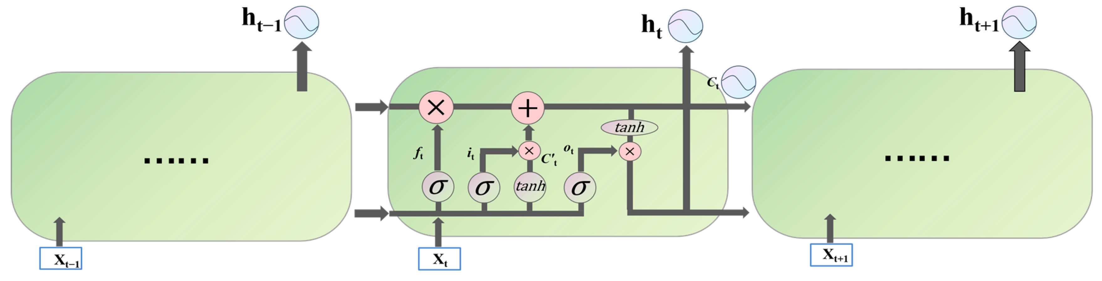
During the day, clouded leopards rest on the trees, which can be regarded as the local search process of the CLA. At that stage, the CLA looks for better solutions around the current solutions. The process can be modeled using Equations (5) and (6); the former can generate random positions near the current position, and the latter compares the value of the two positions and updates the optimal result.

$$x_{i,j}^{P_2}=x_{i,j}^{}+\frac{l_j+r_{i,j}^{}\cdot (u_j-l_j)}{t}\cdot (2r_{i,j}^{}-1)$$

(5)

$$X_i=\{\begin{array}{l}{X}_i^{P_2},F_i^{p_2}<F_i\\ X_i,\hspace{1em}\hspace{1em}\hspace{0.17em}else\end{array}$$

(6)

where $x_{i,j}^{P_2}$ represents the new candidate position of the ith clouded leopard, which is based on the second phase of the CLA; j is the jth decision variable; $F_i^{P_2}$ is the fitness functions value; $r_{i,j}$ is a random number in interval [0, 1].

2.2. LSTM

LSTM is a particular RNN that can effectively solve the problems of gradient explosion and gradient disappearance seen in traditional RNNs [20]. The LSTM unit forms the chain structure of LSTM and the unit is shown in Figure 1.

The LSTM unit contains three gates: forget gate (f_t), input gate (i_t), and output gate (o_t). The forget gate controls the retention of the historical state of time-series data, the input gate controls the input state of information into a cell, and the output gate determines the output value based on the cell state. The process of LSTM can be written as:

$$f_t=\sigma (U_f{x}_t+W_f{h}_{t-1}+b_f)$$

(7)

$$i_i=\sigma (U_i{x}_t+W_i{h}_{t-1}+b_i)$$

(8)

$$C_t^{\prime }=\tanh (U_{C_t^{\prime }}{x}_t+W_{C_t^{\prime }}{h}_{t-1}+b_{C_t^{\prime }})$$

(9)

$$C_t=f_t\times C_{t-1}+i_t\times C_t^{\prime }$$

(10)

$$o_t=\sigma (U_o{x}_t+W_o{h}_{t-1}+b_o)$$

(11)

$$h_t=o_t\times \tanh (C_t)$$

(12)

$$y_t=W_{out}\times h_t+b_{out}$$

(13)

where $U$ and $W$ are learnable weight; $x_t$ is the input of the present phase; $h_{t-1}$ is the output of the previous phase; $b$ is the bias weight.

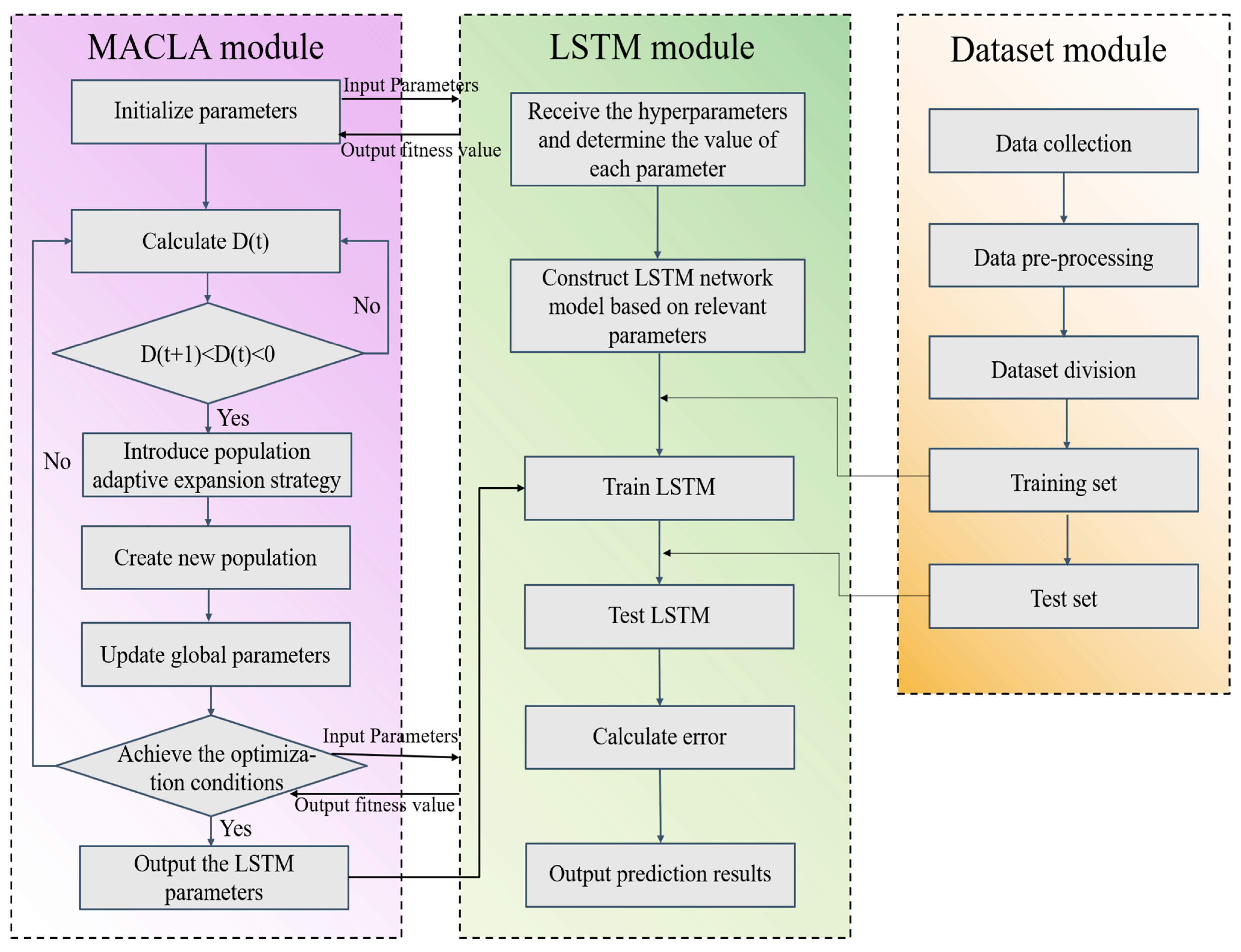
3. Materials and Methods

3.1. Improved CLA Based on a Multiple Adaptive Mechanism

At present, advanced prediction methods based on machine- and deep-learning need a large number of hyperparameters. The selection of these hyperparameters mostly depends on the participants’ subjective experience. It leads to the randomness of the hyperparameters assignment and this often brings a disastrous decline in the model’s generalization performance. Thus, MACLA is investigated to select the hyperparameters, preventing the drastic efficiency drops of the forecasting method seen in off-design situations.

3.1.1. Initialization Based on Chaotic Mapping

Various meta-heuristic optimization algorithms use different initialization methods. The original CLA adopts the following initialization strategy and the parameter Settings of the initialization strategy are shown in

Table 1. Parameter description of initialization.

Parameter	Explanation	Value
$x_{i,j}$	represents jth decision variable of ith clouded leopard	-
N	the total number of clouded leopards	-
m	the number of decision variables	in our study, m = 3
$r_{i,j}$	a random number	in set {0, 1}
$u_j$	the maximum value of decision variables	discussed in the MACLA pseudo-code
$l_j$	the minimum value of decision variables	discussed in the MACLA pseudo-code

:

$$x_{i,j}=l_j+r_{i,j}\cdot (u_j-l_j),i=1,2,\dots N,j=1,2,\dots m$$

(14)

For the CLA, the initial positions of the clouded leopards are a significant constraint in searching for the optimal value. The more homogeneous the initial population in the solution space, the higher the probability that the algorithm will find the optimal value [21]. Thus, a parameter initialization method based on chaotic mapping is considered to replace the random initialization strategy in the CLA. Moreover, it has been proved that chaotic mapping performs better on randomness, ergodicity, and non-repeatability. We compare six chaotic mapping methods, which are commonly used in swarm intelligence. These are shown in

Table 2. Chaotic mapping methods.

Method	Equation	Parameter Value
Logistic	Equation (15)	$u\in [0,4]$
Tent	$x_{k+1}=\{\begin{array}{l}\hspace{0.17em}{x}_k/\beta ,\hspace{1em}\hspace{1em}\hspace{1em}\hspace{1em}{x}_k\in [0,\beta )\\ (1-x_k)/(1-\beta ),\hspace{0.17em}{x}_k\in [\beta ,1]\end{array}$	$\beta \in [0,1]$
Logistic-tent	$x_{k+1}=\{\begin{array}{l}[r{x}_k(1-x_k)+((4-r)x_k)/2]\mathrm{mod}1,\hspace{1em}\hspace{1em}{x}_k\in [0,0.5)\\ [r{x}_k(1-x_k)+((4-r)(1-x_k))/2]\mathrm{mod}1,\hspace{0.17em}{x}_k\in [0.5,1]\end{array}$	$p=0.4$
SPM	$x_{k+1}=\{\begin{array}{c}\mathrm{mod}(x_k/p+\mu \sin (\pi x_k)+r,1),\hspace{1em}\hspace{1em}{x}_k\in [0,p)\\ \mathrm{mod}((x_k/p)/(0.5-p)+\mu \sin (\pi x_k)+r,1),\hspace{1em}\hspace{1em}{x}_k\in [p,0.5)\\ \mathrm{mod}((1-x_k/p)/(0.5-p)+\mu \sin (\pi (1-x_k))+r,1),\hspace{1em}\hspace{1em}{x}_k\in [0.5,1-p)\\ \mathrm{mod}((1-x_k/p)+\mu \sin (\pi (1-x_k))+r,1),\hspace{1em}\hspace{1em}{x}_k\in [1-p,1]\end{array}$	$\begin{array}{l}p=0.4,\mu =0.3,\\ r=\mathrm{rand}(0.1)\end{array}$
Piecewise	$x_{k+1}=\{\begin{array}{c}{x}_k/p,\hspace{1em}\hspace{1em}{x}_k\in [0,p)\\ (x_k-p)/(0.5-p),\hspace{1em}\hspace{1em}{x}_k\in [p,0.5)\\ (1-p-x_k)/(0.5-p),\hspace{1em}\hspace{1em}{x}_k\in [0.5,1-p)\\ (1-x_k)/p,\hspace{1em}\hspace{1em}{x}_k\in [1-p,1]\end{array}$	$p=0.4$
Singer	$x_{k+1}=u(7.86x_k-23.31x_k^2+28.75x_k^3-13.302875x_k^4)$	$u=1$

and the generated distribution of the initial value is shown in Figure 2.

We analyzed the distribution of initial values of the six chaotic mapping methods. The singer chaotic mapping, missing initialization of 0, does not consider the boundary population’s positive effect on the optimization process and its initial distribution is less uniform than other chaotic mapping methods. The tent, Logistic-tent, SPM, and Piecewise have more uniform spatial distribution than the Logistic mapping. However, these chaotic mapping methods do not consider the positive effect of boundary values, which are inspired by clouded leopard hunting behavior. Individuals outside the group have a higher perception ability for prey. Thus, the Logistic is chosen finally, and the mathematical model can be expressed as follows:

$$x_{k+1}=u{x}_k(1-x_k)$$

(15)

where $u$ is the branch parameter; $k$ is the $k$th iteration.

3.1.2. Population Adaptive Expansion

It has been confirmed that premature convergence is closely related to the similarity of individual diversity. The more dispersed the population (diversity increases), the better for the global search; conversely, the more concentrated the population (diversity decreases), the better for the local search [22]. Reasonable deconstructions of the premature convergence phenomenon can improve the efficiency of the optimization algorithm. In order to balance the role of global and local searches in the CLA, the population adaptive expansion strategy is proposed. Specifically, the selection, crossover, and mutation operators from genetic algorithms are introduced into the CLA to enhance the parametric population diversity. The MACLA method uses roulette to select the mutated and crossed individuals. The selected individuals are replicated to produce new populations of individuals. This process realizes the regeneration of population diversity. The increase in population diversity can prevent the optimization algorithm from falling into the local optimal solution and enhance the search ability of the algorithm.

As the algorithm iterates, the range of optimal solutions will shrink. This means that the number of candidate populations decreases. The existing meta-heuristic optimization methods lack the means to assess population diversity. These methods cannot reasonably intervene in the search process and often make themselves fall into the local optimal solution. This paper investigates the population adaptive expansion strategy to tackle the above problem and the population adaptive expansion strategy is given by:

$$D=\frac{2}{N(N-1)}{\displaystyle \sum _{i=1}^{N-1}{\displaystyle \sum _{j=i+1}^{N}d(X_i,X_j}})$$

(16)

$$d_{ij}=\sqrt{{\displaystyle \sum _{K=1}^n{(P_{iK}-P_{jK})}^2}}$$

(17)

where N is the number of population individuals; $X_i\mathrm{and}{X}_j$ are the position vectors of the ith and jth clouded leopards; the position vectors can be expressed as $X_i=\left[P_{i1},P_{i2},\cdots ,P_{in}\right]$, $X_j=\left[P_{j1},P_{j2},\cdots ,P_{jn}\right]$.

The difference between the current and the last diversity evolution result was calculated using Equations (16) and (17). The average Euclidean distance between any two individuals is used to measure population diversity. The distance is positively correlated with the degree of population dispersion. At the early stage of iteration, the convergence speed is fast and the diversity difference in the neighboring iterations is enormous. The diversity difference between the t and the t − 1 iteration is positive. During the iterative procedure, the diversity difference turns negative when the result gradually approaches the optimal solution. In this paper, when the difference is negative for three consecutive times, the population adaptive expansion strategy is introduced to make the result jump out of the local optimal solution.

Specifically, the integration of selection, crossover, and mutation operators from the genetic algorithm is designed to create new populations. In addition, the adaptive diversity weight is proposed to balance the diversity in different iterative processes. Each of these improvements will be described in detail below.

For the genetic algorithm, reproductive individuals are selected by the selection operator. In this paper, roulette wheel selection is used to select the individual clouded leopards that need cross and mutation. This process achieves the establishment of new populations. Roulette wheel selection accumulates sums over the probability of each individual being selected and uses distribution characteristics of random numbers to select the clouded leopards that need cross and mutation. Roulette wheel selection can be expressed as:

$$P(X_i)=\frac{F(X_i)}{{\displaystyle \sum _{i=1}^{N}F(X_i)}}$$

(18)

where $F(X_i)$ is the fitness function value of ith clouded leopard; N is the total number of clouded leopards.

For the genetic algorithms, the probabilities of crossover and mutation operators are usually fixed. The probability of the crossover operator $P_c$ is generally set to $0.3\le P_c\le 0.8$ and the probability of the mutation operators $P_m$ is set to $0.001\le P_m\le 0.1$. However, in the early iteration period, the adaptability of the optimization algorithm is weak and the current adaptability is worse than the average adaptability. Therefore, a large crossover mutation probability is needed to improve the global optimization ability. At this point, the mutation probability should be reduced to preserve local excellent solutions. Furthermore, the probability setting of the late iteration should be opposite to that of the early iteration. The fixed threshold setting will reduce the optimization ability of the algorithm. Therefore, the improved crossover and mutation probability calculation methods are presented:

$$P_c=\{\begin{array}{l}{P}_{c\max },F_{\max }<F_{\mathrm{mean}}\\ P_{c\max }-t\frac{P_{c\max }-P_{c\min }}{t_{\max }},F_{\max }\ge F_{\mathrm{mean}}\end{array}$$

(19)

$$P_m=\{\begin{array}{l}{P}_{m\min },F<F_{\mathrm{mean}}\\ P_{m\min }-t\frac{P_{m\max }-P_{m\min }}{t_{\max }},F\ge F_{\mathrm{mean}}\end{array}$$

(20)

where P represents the probability; F is the fitness functions value; t is the number of current iterations.

This paper tries to prevent the CLA from falling into the local optimal solution through the population adaptive expansion strategy. However, with the continuous iteration of the algorithm, the requirement for population diversity will reduce because of the dispersive property of population diversity. The probability of occurrence of the population adaptive expansion strategy should be adjusted. Therefore, an adaptive diversity weight is designed to balance these probabilities, which can be expressed as:

$$D=\lambda \frac{2}{N(N-1)}{\displaystyle \sum _{i=1}^{N-1}{\displaystyle \sum _{j=i+1}^{N}d(X_i,X_j}})$$

(21)

$$\lambda =\frac{t_{\max }-t}{t_{\max }}$$

(22)

3.1.3. Adaptive Step Size Search Parameters

The CLA uses Equations (3) and (5) for the global and local optimal search, respectively. It uses random values r to update the superior values around the current results. This strategy is stochastic, which highly affects the performance of the optimization algorithm. It is well known that the optimal value should be progressively closer to the current iteration result as the iteration proceeds. Thus, we consider an adaptive step size search parameter strategy to balance the search range of the parameters in the early and late iterations. The proposed strategy can perform a large range of optimal value searches in the early iterations and a small range of optimal value searches in the late iterations. The random function $r_p$ of this strategy can be written as Equation (23), in which it replaces the random parameters in Equations (3) and (5).

$$r_p=r\frac{t_{\max }-t}{t_{\max }}$$

(23)

where $r$ is a random number in interval [0, 1].

3.2. MACLA-LSTM

The water demand is affected by temperature, humidity, geography, and other factors. The combination of multiple factors makes forecasting more difficult. In this paper, the LSTM is used as the basic model. However, the LSTM has multiple hyperparameters, such as the window size, the batch size, and the number of hidden layers. These hyperparameters are selected by the subjective experience of the researchers; however, it often leads to a decline in prediction accuracy. Thus, the MACLA-LSTM is proposed. We consider the value range of the above three hyperparameters as the initial group and the MACLA is applied to obtain the optimal parameter combination. Then, the output of the MACLA are taken as the input parameter of the LSTM.

The MACLA-LSTM can be divided into three parts: the MACLA module, the LSTM module, and the dataset module. The pseudo-code of the MACLA is shown in the following Algorithm 1:

Algorithm 1: MACLA

Input: X(w,b,n), the range of time window size (w), batch size (b), and the number of hidden layers (n) of the LSTM; Max initialization: number of initialization iterations; Max iteration: number of iterations Output: the optimal combination of time window size, batch size, and number of hidden layers parameters 1: X: w = [1, 100]; b = [1, 50]; n = [1, 5]; 2: while (t < Max initialization) do 3:   $X(t+1)=uX(t)(1-X(t))$; 4: end 5: $\lambda ,r_p\leftarrow 0$ 6: while (current iteration < Max iteration) do 7:    while (i < N−1) do 8:       if $D=\lambda \frac{2}{N(N-1)}{\displaystyle \sum _{i=1}^{N-1}}{\displaystyle \sum _{i=i+1}^N}d(X_i,X_j)$< 0 do 9:$X=X_{\mathrm{expand}}$$\text{\#} X_{\mathrm{expand}}$ is the result of population adaptive expansion#  10:      end if 11:    end  12:    while (I < N−1) do 13:        $F_i=MAE(X_i)+MSE(X_i)$ 14:       if $F_i^{P_1}<F_i$ do 15:           $X_i=X_i^{P_1}$ 16:      else 17:$X_i=X_i^{}$ 18:        end if 19:        if $F_i^{P_2}<F_i$ do 20:           $X_i=X_i^{P_2}$ 21:        else 22:$X_i=X_i^{}$ 23:        end if 24:        $F_i=MAE(X_i)+MSE(X_i)$ 25:        $currentiteration=currentiteration+1$ 26:        end 27: end 28: Generate the optimal combination of time window size, batch size and number of hidden layers parameters Note: The content after # is a further explanation of the current content.

The main steps of the water demand prediction based on the MACLA-LSTM model are as follows, and a diagram of the MACLA-LSTM is shown in Figure 3.

Step 1: Initialize the parameters of MACLA;

Step 2: Calculate population diversity to determine whether the MACLA falls into the local optimal solution. If so, introduce the population adaptive expansion strategy. Otherwise, return to the previous step;

Step 3: Determine whether the current solution is the optimal solution. If so, update the LSTM parameters. Otherwise, return to Step 2;

Step 4: Train the LSTM model and predict water demand.

4. Experiment

4.1. Evaluation Metrics

The mean squared error (MSE), the coefficient of determination (R²), and the mean absolute error (MAE) are used to evaluate the MACLA-LSTM [23]. These evaluation metrics are formulated as follows:

$$\mathrm{MSE}=\frac{1}{N}{\displaystyle \sum _{i=1}^N{(y_i-{\widehat{y}}_i)}^2}$$

(24)

$${\mathrm{R}}^2=1-\frac{{\displaystyle \sum _{i=1}^N{(y_i-{\widehat{y}}_i)}^2}}{{\displaystyle \sum _{i=1}^N{(y_i-{\overline{y}}_i)}^2}}$$

(25)

$$\mathrm{MAE}=\frac{1}{N}{\displaystyle \sum _{i=1}^N\left|y_i-{\widehat{y}}_i\right|}$$

(26)

where N represents the length of test data; $y_i$ is the ground truth value; $\widehat{y}$ is the forecasted value; and, ${\overline{y}}_i$ is the mean of the ground truth value.

4.2. Experimental Setting

The experiments were carried out in a Windows 10 system with an NVIDIA GeForce RTX 3080 graphics card, which has 10 GB memory; the CPU is 11th Gen. Intel Core i7-11700. The programming language is Python.

4.3. Analysis of the MACLA Effect

In this section, we test the effect of the MACLA to verify the effectiveness of the improvements. Four different fitness functions are used in these experiments. Furthermore, each experiment starts with the initial clouded leopard population and carries out 20 iterations. The fitness value of each iteration is recorded and the results are shown in Figure 4.

The four fitness functions are as follows:

$$F_1(x)=\max \left\{\left|x_i\right|\right\}$$

(27)

$$F_2(x)={\displaystyle \sum _{i=1}^m\left|x_i\right|}+{\displaystyle \prod _{i=1}^m\left|x_i\right|}$$

(28)

$$F_3(x)={\displaystyle \sum _{i=1}^m{x}_i^2}$$

(29)

$$F_4(x)={\displaystyle \sum _{i=1}^m-x_i}\sin (\sqrt{\left|x_i\right|})$$

(30)

These results show that the MACLA can achieve a continuous search and jump out of the local optimal solution more easily than the primary method and the MACLA has higher efficiency in the optimization process. Overall, the MACLA performance has been dramatically improved.

Moreover, we compared the performance of the MACLA with the current mainstream intelligent optimization algorithms: the Marine Predators Algorithm (MPA) [25], Tunicate Swarm Algorithm (TSA) [26], and the Whale Optimization Algorithm (WOA) [27]. The parameter values of each comparison algorithm are shown in

Table 3. Parameter values for the competitor algorithms.

Method	Parameter	Value
MPA	Constant number	p = 0.5
	Random vector	R is a vector of uniform random numbers from [0, 1]
	Fish aggregating devices (FADs)	FADs = 0.2
	Binary vector	U = 0 or 1
TSA	Pmin and Pmax	Pmin = 1, Pmax = 4
	C1, C2, C3	random numbers lie in the range [0, 1]
WOA	Convergence parameter (a)	Linear reduction from 2 to 0
	Random vector (r)	In [0, 1]
	Random number (l)	In [−1, 1]

. And the

Table 4. Optimization results of MACLA and competitor algorithms on test functions.

F		MACLA	MPA	TSA	WOA
F1([−100, 100])	Mean	0	3.17 × 10−19	0.0038	27.7122
	Best	0	7.30 × 10−20	4.42 × 10−5	2.5181
	Worst	0	6.32 × 10−19	0.0278	68.2198
	Std	0	1.70 × 10−19	0.0066	23.1465
	Median	0	2.81 × 10−19	0.0012	24.7617
	ET	1.7862	2.2537	1.2056	0.5108
	Rank	1	2	3	4
F2([−10, 10])	Mean	0	5.98 × 10−28	3.10 × 10−28	6.51 × 10−104
	Best	0	3.57 × 10−30	2.30 × 10−10	1.07 × 10−113
	Worst	0	2.76 × 10−27	8.19 × 10−28	1.21 × 10−102
	Std	0	8.19 × 10−28	2.71 × 10−28	2.28 × 10−103
	Median	0	2.61 × 10−29	7.08 × 10−29	5.72 × 10−107
	ET	2.1056	2.7646	1.4123	0.5983
	Rank	1	4	3	2
F3([−100, 100])	Mean	0	9.61 × 10−50	3.89 × 10−46	2.11 × 10−153
	Best	0	9.42 × 10−53	4.13 × 10−50	3.02 × 10−168
	Worst	0	7.76 × 10−49	3.11 × 10−44	3.72 × 10−152
	Std	0	2.51 × 10−49	2.56 × 10−45	4.41 × 10−153
	Median	0	2.87 × 10−50	6.76 × 10−48	7.21 × 10−157
	ET	1.7856	2.4564	1.4501	0.5691
	Rank	1	3	4	2
F4([−500, 500])	Mean	−10,312.3	−9571.9	−5909.3	−8624.4
	Best	−12,412.1	−11,341.2	−7198.0	−10,128.2
	Worst	−8123.4	−9012.3	−5012.3	−7527.2
	Std	1569.7	547.2	589.7	699.3
	Median	−11,002.2	−9578.1	−6102.4	−9184.5
	ET	2.8721	2.7671	1.7652	0.9752
	Rank	1	2	4	3

shows the results of various intelligent optimization algorithms on different fitness functions, which proves the excellent performance of MACLA.

4.4. Analysis of MACLA-LSTM Effect

4.4.1. Data and Preprocessing

In our experiments, we used the previous 72 h of water demand as input to predict the water demand for the next 24 h. The short-term forecasting methods use short-term data as input to predict a specific phase (the phase is less than the time of the input). The long-term forecasting method predicts long-period data in the future by increasing the input data time. Compared to short-term forecasting methods, long-term forecasting methods need to focus more on the periodicity and trend of the time series. For short-term water demand forecasting methods, many characteristic values such as temperature, humidity, and wind speed introduce more fluctuations over a long period and do not provide a clear and stable short-term impact; moreover, long-term observation of such meteorological data is not economical and feasible. Therefore, the water demand is the only input in this paper. The dataset is constructed based on the water demand of departments, companies, and mall scenarios in a case study of a metropolitan government in central China. For department data, most users are residents, and for company and mall data, the users are commercial. The dataset collected hourly water consumption data for each scenario from 1 January 2021, to 6 July 2022 and these data are divided into training and testing datasets by 8:2. For abnormal data (extremely large or negative data), we use the average of adjacent periods to correct. In

Table 5. Basic information of the data.

Date	Current Recording Time	Current Cumulative Water Consumption	Last Recorded Time	Last Cumulative Water Consumption	Water Demand (m3)
6 July 2022 07:00	6 July 2022	273,342.280	6 July 2022	273,330.640	11.640
6 July 2022 06:00	6 July 2022	273,330.640	6 July 2022	273,319.000	11.640
6 July 2022 05:00	6 July 2022	273,319.000	6 July 2022	273,309.000	10.000
6 July 2022 04:00	6 July 2022	273,309.000	6 July 2022	273,299.530	9.470
6 July 2022 03:00	6 July 2022	273,299.530	6 July 2022	273,287.100	12.430
6 July 2022 02:00	6 July 2022	273,287.100	6 July 2022	273,270.300	16.800
6 July 2022 07:00	6 July 2022	273,342.280	6 July 2022	273,330.640	11.640
……	……	……	……	……	……
1 January 2021 13:00	1 January 2021	15,406.443	26 April 2021	15,386.870	19.573
1 January 2021 12:00	1 January 2021	15,386.870	26 April 2021	15,364.255	22.615
1 January 2021 11:00	1 January 2021	15,364.255	26 April 2021	15,341.004	23.251
1 January 2021 10:00	1 January 2021	15,341.004	26 April 2021	15,318.378	22.626
1 January 2021 09:00	1 January 2021	15,318.378	26 April 2021	15,295.885	22.493
1 January 2021 08:00	1 January 2021	15,295.885	26 April 2021	15,271.406	24.479
1 January 2021 07:00	1 January 2021	15,271.406	26 April 2021	15,249.089	22.317

, we present part of the experimental data.

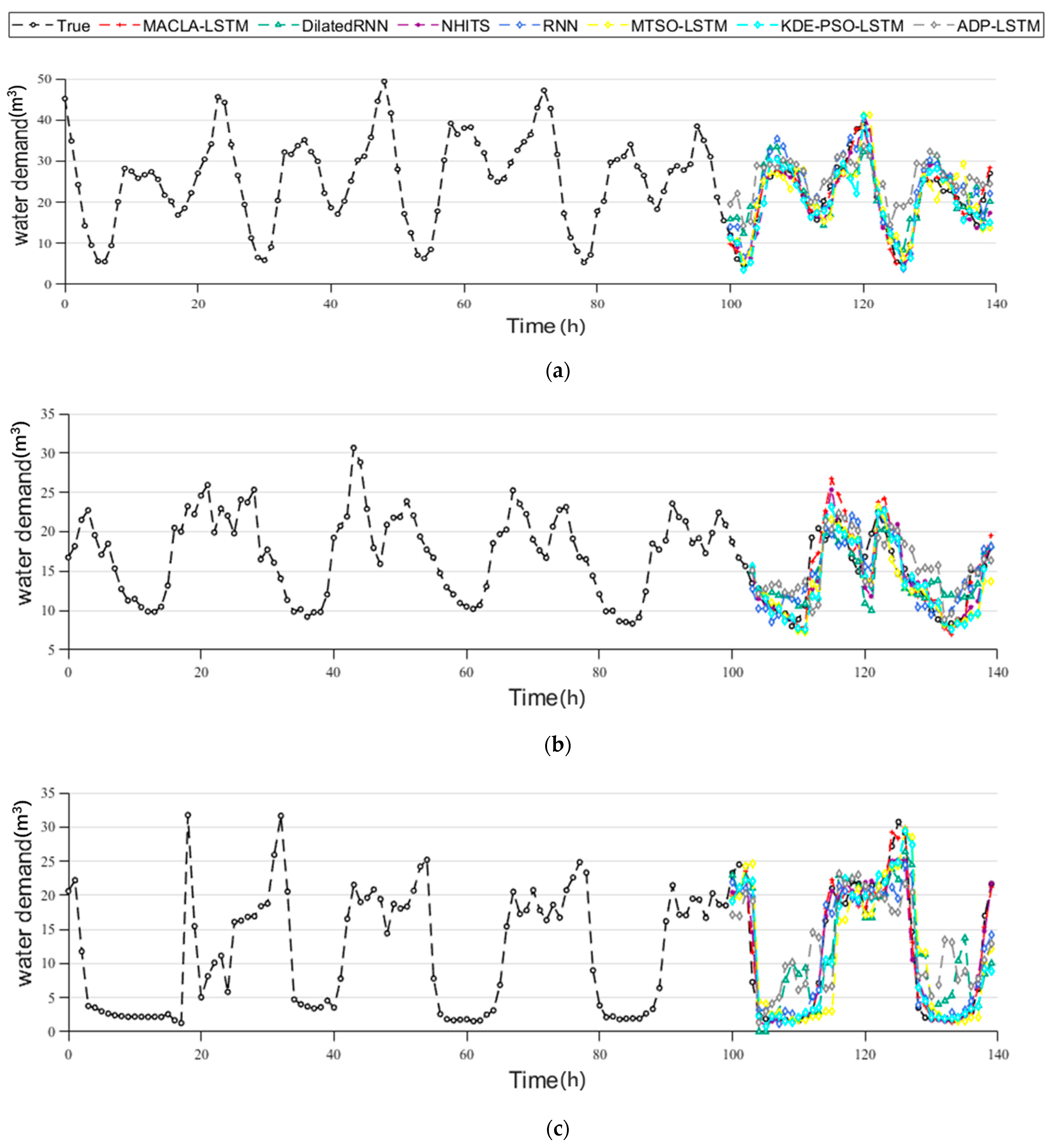
4.4.2. Results Analysis

Dilated RNN [16], NHITS [24], classical RNN [15], MTSO-LSTM [23], ADP-LSTM [24], and KDE-PSO-LSTM [28] models are used to compare the prediction effect with the MACLA-LSTM model and the comparison results are shown in Figure 5. Figure 5 shows the comparison results of the seven prediction models in the three scenarios from 1 May 2021 to 6 May 2021. The horizontal coordinate of the figure represents the time node and the time interval is 1 h. The vertical coordinate represents the value of water demand.

The results show that the predicted trends of the seven models in the three scenarios are consistent with the actual data trend and the fitting degree of the RNN model is significantly lower than the others. The main reason is that the RNN model cannot solve the modeling problem of long sequences. This problem results in the inability to extract long-dimensional features accurately. In addition, the fitting degree of the Dilated RNN and the NHITS is close. The NHITS improves upon the NBEATS [25] to make the model suitable for long-time prediction tasks. For the NHITS, the hierarchical sub-sampling and interpolation method is used to alleviate the problem of low prediction efficiency and accuracy with increased prediction length. Multi-rate data sampling and interpolation methods are used in NHITS and NBEATS. Although these methods help reduce the calculation amount of the models, it also leads to the loss of data features. Therefore, the NHITS has achieved poorer results than the MACLA-LSTM. The Dilated RNN introduces dilated recurrent skip connections and multiple expansion cycle layer structures based on the RNN model. These improvements allow the model to learn multi-dimensional dependencies with fewer parameters. As expected, Dilated RNN achieves better prediction results than the RNN on our dataset; however, it also cannot overcome the long sequence-dependent modeling problem in the RNN.

The MTSO-LSTM, ADP-LSTM, and KDE-PSO-LSTM were proposed in recent years. These methods combine the advantage of intelligent optimization algorithms with LSTM and achieved excellent performance in prediction tasks in various fields. We modified the above methods to make them suitable for water demand forecasting tasks.

The MTSO-LSTM proposed a hybrid prediction model containing the modified tuna swarm optimization and the LSTM prediction model. The improved modified tuna swarm optimization is used to perform hyperparameter screening of the LSTM. The LSTM model uses the decomposed wind speed data as input to achieve wind speed prediction. This paper uses the complete water demand data, replacing the decomposed data, as input.

Similarly, the ADP-LSTM uses the adaptive dynamic particle swarm optimization algorithm to obtain the optimal LSTM hyperparameters. The KDE-PSO-LSTM is a recently published method for water demand prediction. The method combines LSTM to kernel density estimation, optimized by using the particle swarm optimization algorithm. Moreover, the KDE-PSO-LSTM corrects the predicted data by calculating the difference between the corrected predicted and actual values. The results show that KDE-PSO-LSTM has better prediction performance than MTSO-LSTM and ADP-LSTM; however, its computational cost is also further increased. Both methods use LSTM as a prediction model, and the MACLA-LSTM has the best prediction accuracy, further indicating the advantage of MACLA for hyperparameter searches.

Table 6. Experimental results of different models, ⬆: the higher the better; ⬇: the lower the better.

Method	MAE ⬇	MSE ⬇	R2 (%) ⬆
RNN [15]	3.69	18.52	95.91
	3.31	17.48	96.03
	2.64	15.14	93.69
NHITS [24]	2.11	8.12	97.55
	1.41	3.80	98.26
	1.61	5.70	97.62
Dilated RNN [16]	2.36	8.97	95.60
	2.28	8.01	96.33
	2.83	9.45	95.81
MTSO-LSTM [23]	2.52	7.62	96.08
	2.37	8.04	96.52
	1.97	7.47	94.97
ADP-LSTM [24]	4.76	8.65	94.81
	5.01	9.16	93.29
	5.64	10.22	92.71
KDE-PSO-LSTM [28]	1.41	3.89	97.65
	1.28	2.16	97.91
	1.22	3.08	96.21
MACLA-LSTM	1.12	2.22	99.51
	0.89	1.21	99.44
	1.09	2.38	99.01

shows the evaluation results of each method’s global average forecasting accuracy. For the company dataset, the MACLA-LSTM generated 0.89 MAE, 1.21 MSE, and 99.44 R², which significantly improves the prediction accuracy compared with other models. In other scenarios, the MACLA-LSTM also has the highest prediction accuracy; moreover, we noticed that the accuracy of the department dataset is lower than in other scenarios. This is mainly due to the fact that the water demand of the departments is highly volatile because of other external elements.

In the three-scenario dataset, MACLA-LSTM obtains the best-fitting curve and prediction accuracy, which proves its validity and reliability. Therefore, MACLA-LSTM can be used as an efficient and reliable prediction model for water demand forecasting in different scenarios.

5. Conclusions

This paper presents a theoretical and experimental study for short-term prediction water demand forecasting, aiming to enhance the effective management of urban water supply. The proposed MACLA-LSTM can fully combine the hyperparameter adjustment ability of MACLA and the prediction advantage of the LSTM model. The validity of the MACLA-LSTM is verified on a real-water-demand dataset. The MACLA-LSTM achieved MAE values of 1.12, 0.89, and 1.09; MSE values of 2.22, 1.21, and 2.38; and R2 values of 99.51%, 99.44%, and 99.01%. Compared with other methods, the prediction accuracy is significantly improved. Overall, the MACLA-LSTM method, with limited computational cost, improves prediction accuracy by optimizing the hyperparameter input of the LSTM model. Despite its preliminary character, this study can indicate the feasibility of the deep learning method in water demand forecasting tasks.

However, the field still faces many challenges. According to current research, deep learning methods have been applied in many urban water demand forecasting models but they have certain limitations. For example, these methods have insufficient prediction accuracy in long-term forecasting tasks. It is difficult to integrate valid information under multi-factor environmental variables. Therefore, it is a challenge to explore a long-term water demand forecasting model that can address multi-factor environmental variables. In addition, the interpretability of predictive models is also a major challenge.

Nevertheless, the MACLA-LSTM method has achieved good prediction accuracy in short-term water demand forecasting tasks. The MACLA-LSTM is hoped to be applied to more prediction tasks, especially long-term prediction tasks in the future.

References

1. Choi, H.; Suh, S.; Kim, S.; Han, E.J.; Ki, S.J. Assessing the Performance of Deep Learning Algorithms for Short-Term Surface Water Quality Prediction. Sustainability 2021, 13, 10690. [Google Scholar] [CrossRef]
2. Xu, Z.; Lv, Z.; Li, J.; Shi, A. A novel approach for predicting water demand with complex patterns based on ensemble learning. Water Resour. Manag. 2022, 36, 4293–4312. [Google Scholar] [CrossRef]
3. Niu, Z.; Wang, C.; Zhang, Y.; Wei, X.; Gao, X. Leakage rate model of urban water supply networks using principal component regression analysis. Trans. Tianjin Univ. 2018, 24, 172–181. [Google Scholar] [CrossRef]
4. Olsson, G. Urban water supply automation–today and tomorrow. J. Water Supply Res. Technol. -AQUA 2021, 70, 420–437. [Google Scholar] [CrossRef]
5. Kozłowski, E.; Kowalska, B.; Kowalski, D.; Mazurkiewicz, D. Water demand forecasting by trend and harmonic analysis. Arch. Civ. Mech. Eng. 2018, 18, 140–148. [Google Scholar] [CrossRef]
6. Luna, T.; Ribau, J.; Figueiredo, D.; Alves, R. Improving energy efficiency in water supply systems with pump scheduling optimization. J. Clean. Prod. 2019, 213, 342–356. [Google Scholar] [CrossRef]
7. Xu, W.; Chen, J.; Zhang, X.J. Scale effects of the monthly streamflow prediction using a state-of-the-art deep learning model. Water Resour. Manag. 2022, 36, 3609–3625. [Google Scholar] [CrossRef]
8. Sherstinsky, A. Fundamentals of recurrent neural network (RNN) and long short-term memory (LSTM) network. Phys. D Nonlinear Phenom. 2020, 404, 132306. [Google Scholar] [CrossRef] [Green Version]
9. Chen, Z.; Ma, Q.; Lin, Z. Time-Aware Multi-Scale RNNs for Time Series Modeling. In Proceedings of the Thirtieth International Joint Conference on Artificial Intelligence (IJCAI-21), Montreal, QC, Canada, 19–27 August 2021; pp. 2285–2291. [Google Scholar]
10. Chang, S.; Zhang, Y.; Han, W.; Yu, M.; Guo, X.; Tan, W.; Cui, X.; Witbrock, M.; Hasegawa-Johnson, M.A.; Huang, T.S. Dilated recurrent neural networks. Adv. Neural Inf. Process. Syst. 2017, 30, 1–11. [Google Scholar]
11. Yu, Y.; Si, X.; Hu, C.; Zhang, J. A review of recurrent neural networks: LSTM cells and network architectures. Neural Comput. 2019, 31, 1235–1270. [Google Scholar] [CrossRef]
12. Nasser, A.A.; Rashad, M.Z.; Hussein, S.E. A two-layer water demand prediction system in urban areas based on micro-services and LSTM neural networks. IEEE Access 2020, 8, 147647–147661. [Google Scholar] [CrossRef]
13. Zanfei, A.; Brentan, B.M.; Menapace, A.; Righetti, M.; Herrera, M. Graph convolutional recurrent neural networks for water demand forecasting. Water Resour. Res. 2022, 58, e2022W–e32299W. [Google Scholar] [CrossRef]
14. Li, W.; Wang, G.; Gandomi, A.H. A survey of learning-based intelligent optimization algorithms. Arch. Comput. Method. Eng. 2021, 28, 3781–3799. [Google Scholar] [CrossRef]
15. Kim, C.; Batra, R.; Chen, L.; Tran, H.; Ramprasad, R. Polymer design using genetic algorithm and machine learning. Comp. Mater. Sci. 2021, 186, 110067. [Google Scholar] [CrossRef]
16. Grefenstette, J.J. Genetic algorithms and machine learning. In Proceedings of the Sixth Annual Conference on Computational Learning Theory, Santa Cruz, CA, USA, 26–28 July 1993; pp. 3–4. [Google Scholar]
17. Naik, A.; Satapathy, S.C. Past present future: A new human-based algorithm for stochastic optimization. Soft Comput. 2021, 25, 12915–12976. [Google Scholar] [CrossRef]
18. Rumelhart, D.E.; Hinton, G.E.; Williams, R.J. Learning representations by back-propagating errors. Nature 1986, 323, 533–536. [Google Scholar] [CrossRef]
19. Yang, F.; Wang, P.; Zhang, Y.; Zheng, L.; Lu, J. Survey of swarm intelligence optimization algorithms. In Proceedings of the 2017 IEEE International Conference on Unmanned Systems (ICUS), Beijing, China, 27–29 October 2017; pp. 544–549. [Google Scholar]
20. Attiya, I.; Abd Elaziz, M.; Abualigah, L.; Nguyen, T.N.; Abd El-Latif, A.A. An improved hybrid swarm intelligence for scheduling iot application tasks in the cloud. IEEE T. Ind. Inform. 2022, 18, 6264–6272. [Google Scholar] [CrossRef]
21. Bharathi, P.; Ramachandran, M.; Ramu, K.; Chinnasamy, S. A Study on Various Particle Swarm Optimization Techniques used in Current Scenario. Des. Model. Fabr. Adv. Robot. 2022, 1, 15–26. [Google Scholar]
22. Song, G.; Zhang, Y.; Bao, F.; Qin, C. Stock prediction model based on particle swarm optimization LSTM. J. Beijing Univ. Aeronaut. Astronaut. 2019, 45, 2533–2542. [Google Scholar]
23. Tuerxun, W.; Xu, C.; Guo, H.; Guo, L.; Zeng, N.; Cheng, Z. An ultra-short-term wind speed prediction model using LSTM based on modified tuna swarm optimization and successive variational mode decomposition. Energy Sci. Eng. 2022, 26, 105804. [Google Scholar] [CrossRef]
24. Zhang, G.; Tan, F.; Wu, Y. Ship motion attitude prediction based on an adaptive dynamic particle swarm optimization algorithm and bidirectional LSTM neural network. IEEE Access 2020, 8, 90087–90098. [Google Scholar] [CrossRef]
25. Faramarzi, A.; Heidarinejad, M.; Mirjalili, S.; Gandomi, A.H. Marine Predators Algorithm: A nature-inspired metaheuristic. Expert Syst. Appl. 2020, 152, 113377. [Google Scholar] [CrossRef]
26. Kaur, S.; Awasthi, L.K.; Sangal, A.L.; Dhiman, G. Tunicate Swarm Algorithm: A new bio-inspired based metaheuristic paradigm for global optimization. Eng. Appl. Artif. Intel. 2020, 90, 103541. [Google Scholar] [CrossRef]
27. Mirjalili, S.; Lewis, A. The whale optimization algorithm. Adv. Eng. Softw. 2016, 95, 51–67. [Google Scholar] [CrossRef]
28. Du, B.; Huang, S.; Guo, J.; Tang, H.; Wang, L.; Zhou, S. Interval forecasting for urban water demand using PSO optimized KDE distribution and LSTM neural networks. Appl. Soft Comput. 2022, 122, 108875. [Google Scholar] [CrossRef]
Figure 1. LSTM unit structure.
Sustainability 15 03628 g001
Figure 2. Distribution of initial value. (a) Logistic. (b) Tent. (c) Logistic-tent. (d) SPM. (e) Piecewise. (f) Singer.
Sustainability 15 03628 g002
Figure 3. MACLA-LSTM module.
Sustainability 15 03628 g003
Figure 4. Optimization results of different fitness functions. (a) F1. (b) F2. (c) F3. (d) F4.
Sustainability 15 03628 g004aSustainability 15 03628 g004b
Figure 5. Visualization of forecasting results in different scenarios. (a) Department. (b) Company. (c) Mall.
Sustainability 15 03628 g005