Abstract
Interferometric Synthetic Aperture Radar (InSAR) has proved its efficiency for displacement monitoring in urban areas. However, the large volume of data generated by this technology turns the retrieval of information useful for structure monitoring into a big data problem. In this study, a new tool (SARClust) to analyze InSAR displacement time series is proposed. The tool performs the clustering of persistent scatterers (PSs) based on dissimilarities between their displacement time series evaluated through dynamic time warping. This strategy leads to the formation of clusters containing PSs with similar displacements, which can be analyzed together, reducing data dimensionality, and facilitating the identification of displacement patterns potentially related to structural damage. A proof of concept was performed for downtown Lisbon, Portugal, where ten distinct displacement patterns were identified. A relationship between clusters presenting centimeter-level displacements and buildings located on steep slopes was observed. The results were validated through visual inspections and comparison with another tool for time series analysis. Agreement was found in both cases. The innovation in this study is the attention brought to SARClust’s ability to (i) analyze vertical and horizontal displacements simultaneously, using an unsupervised procedure, and (ii) characterize PSs assisting the displacement interpretation. The main finding is the strategy to identify signs of structure damage, even on isolated buildings, in a large amount of InSAR data. In conclusion, SARClust is of the utmost importance to detect potential signs of structural damage in InSAR displacement time series, supporting structure safety experts in more efficient and sustainable monitoring tasks.
1. Introduction
Interferometric Synthetic Aperture Radar (InSAR) is a remote sensing method for displacement measurement from satellite images which enables observations at points naturally existing on the Earth surface through cloud cover, during both day and night. The usage of multiple images allows displacement measurement every few days (often less than a week) and millimeter precision. Monitoring displacements in urban areas is a key task to assure the safety of its inhabitants, workers, and visitors. InSAR has been widely applied for this purpose in order to evaluate subsidence, settlements, landslides or seasonal behavior [1,2,3,4,5,6,7]. In an urban environment, where natural reflectors are abundant, this technique may provide hundreds or even thousands of measurement points per km2. Furthermore, the SAR image archives currently available enable assessment to hundreds of displacement observation epochs for each point. The large volume of data achieved and the direction of the observed displacements (along the sensor line-of-sight—LOS), turns the interpretation of the displacement time series into a difficult task for InSAR non-experts, as is often the case for structure engineers. The retrieval of information from the displacement time series is particularly important when applied to structure monitoring. Structures react to loads they are subjected to and often present non-linear displacements due to variations of those loads (e.g., temperature). In cases where the structure is affected by some damage, its reaction will present a displacement anomaly. Therefore, displacement time series are important to assist structure experts in the identification of possible structural damages.
The growing availability of SAR datasets with larger spatial and temporal resolutions make the development of techniques to extract information from InSAR displacement time series (called radar interpretation) more pressing. The fitting of regression models has been used for InSAR displacement time series analysis, enabling the mapping of the spatial distribution of regression coefficients to identify different displacement patterns [6,8]. The definition of deviation indices that quantify changes between subsets of displacement time series has been used to detect measurement points with anomalous displacements [9,10]. Cluster analysis has been applied either to ground motion characterization or to the detection of outlier measurement points [11,12]. Displacement time series classification according to a library of predefined displacement models has been performed through sequential hypothesis testing, which allows for the detection of displacement anomalies [13,14]. Some authors have also proposed the combination of several of the above methods to achieve improved results [15,16]. Artificial intelligence has been used not only for displacement time series analysis [17,18,19], but also to evaluate deformation patterns in interferograms [20,21,22]. The exploration of InSAR time series through artificial intelligence has also been used to mitigate uncertainty sources of the data, such as atmospheric effects [23,24,25] or unwrapping errors [26]. Two recent trends in this field are the separation of effects coming from different sources [27,28] and the prediction of future InSAR observations [29,30].
In this study, a new tool for semiautomatic analysis of InSAR displacement time series is presented, called SARClust—Clustering of InSAR displacement time series. The tool forms clusters of InSAR measurement points with homogeneous behavior. This means the points in each cluster present similar displacement time series among themselves, but different from the displacement time series of the points in other clusters. This strategy reduces the InSAR data dimensionality; clusters become the unit for analysis, which facilitates the identification of spatiotemporal patterns in the displacements and, consequently, the detection of possible anomalies in the displacement time series. Displacement time series representative of each cluster behavior are computed, and auxiliary data can be inputted to the tool in raster format to assist cluster characterization and interpretation. SARClust uses a hierarchical clustering approach for cluster analysis [31] in which distances between displacement time series determined through dynamic time warping are used as the dissimilarity measure [32]. Displacements from different observation geometries, i.e., from ascending and descending passes of SAR satellites, are combined and the clusters are built considering both vertical and horizontal displacements. In this study, a proof of concept is performed for downtown Lisbon, Portugal, where the tool is used to detect eventual anomalies in the displacement time series of measurement points located on heritage buildings from the 18th century. Ten clusters of distinct structural behavior are identified. Two of those clusters present small magnitude displacements during the time of analysis, suggesting the buildings where the points in those clusters are located did not present signs of damages. However, the remaining clusters present anomalies on their displacement time series. Some of the clusters in this last group present centimeter-level displacements and are associated with buildings located on steep slopes. Visual inspections confirm the presence of damage on those buildings. The results show that SARClust is an efficient tool to assist structure monitoring in detecting anomalies in InSAR displacement time series.
2. Materials and Methods
2.1. Study Area
The study area was downtown Lisbon, in Portugal (Figure 1). The downtown area is located at the northern bank of Tagus River, at the junction point of two old streams (now piped), and it is built on alluvial soil. It is a flat area, with slopes mainly below 5°, flanked by hills formed by sand, limestone and clay. The hills present large slopes, reaching 26° at some locations. In 1755, Lisbon was hit by an Mw 8.7 earthquake, followed by a tsunami. Due to the ground properties and to its proximity to the river, the downtown area suffered severe damage from the double disaster and was rebuilt. The renewed downtown brought improvements to both urbanism and building design. The new area was organized into large and perpendicular streets (Figure 1c) to allow efficient responses to future disasters. The new buildings followed a homogeneous style, containing timber structures (called “gaiolas pombalinas”) inside masonry walls, that increased their resistance to earthquakes. In the present day, downtown Lisbon is a cultural heritage site, almost 270 years old, that reflects the state of the art of urban planning and building construction in the 18th century and requires frequent monitoring for damage detection at an early stage and timely maintenance.
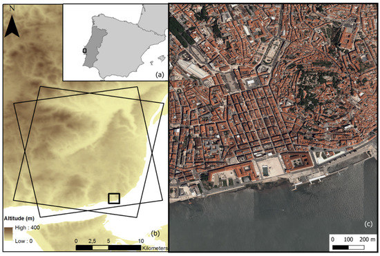
Figure 1.
Study area: (a) location of Lisbon (black rectangle) in Portugal; (b) digital elevation model at Lisbon region—the large rectangles are the areas for Persistent Scatterer Interferometry processing in ascending and descending passes, and the small rectangle is the downtown area; (c) aerial orthophotograph of the downtown area provided by the Portuguese National System for Geographical Information.
2.2. Data Sources
Displacements on Lisbon were determined through SAR images from the sensor on board of European Space Agency (ESA) satellite Sentinel-1A, acquired in TOPSAR mode between March 2015 and February 2018, every 12 days. Two datasets were considered: one from an ascending and another one from a descending pass of the satellite. The dataset from the ascending pass had the relative orbit 45. The incidence angle was 40.6° and the satellite heading was −10.5°. The descending dataset was from the relative orbit 125, with an incidence angle of 35.7° and a heading of 190.5°. The polarization was VV for both datasets and precise orbits were considered. The ascending dataset contained 89 images and the descending one had 86. The used digital elevation model (DEM) was the European DEM (EU-DEM), provided by the European Environment Agency (EEA). All these data are freely available through the Copernicus program.
2.3. Methods for Data Processing and Displacement Detection
The proposed methodology is divided in two parts: the first part is the determination of displacement time series through a multitemporal InSAR technique; the second part is the core of SARClust, i.e., the clustering of the InSAR measurement points based on the similarities of their displacement time series.
2.3.1. PSI Analysis
InSAR displacement time series are determined from a stack of SAR images through the Persistent Scatterer Interferometry (PSI) algorithm implemented in SARPROZ© [33]. The software selects the image that minimizes both temporal and perpendicular baselines as reference. The remaining images are coregistered with respect to the reference one. A ground control point is manually selected to geocode the stack of SAR images and a DEM is used to estimate and remove the topographic component of the phase. The atmospheric phase screen (APS) is estimated for a selection of points with large amplitude stability, interpolated for the whole processed area and removed from phase. Candidates to Persistent Scatterers (PSs) are selected and cumulative displacement together with residual height are estimated for each of them, according to a certain displacement model. As this study intends to evaluate structure behavior, which is usually non-linear, a non-linear displacement model, such as that applied in Milillo et al. [34], is used. Displacement time series are also determined for each PS, with a displacement observation for each SAR image acquisition epoch.
In this study, an area of 16 km × 16 km of Lisbon metropolitan area (Figure 1b) was considered to test the proposed methodology. The SAR images from the ascending and descending passes considered in this study were processed in SARPROZ© independently. Therefore, two distinct sets of PSs were achieved, each of them associated with time series of displacements along the LOS direction of each pass. Observation epochs were also different for both datasets. The reference points for the ascending and descending datasets were not coincident but were both located far from the downtown area. Only measurement points with temporal coherence greater than or equal to 0.9 were considered as PSs and used for further analysis.
2.3.2. Selection of PSs on Buildings
Although PSI was applied on a large area of Lisbon metropolitan area for improved orbit and APS estimation, SARClust was tested only for the downtown area—for an area of approximately 1 km2. Furthermore, the analysis was performed only for PSs located on buildings, in order to exclude points in objects such as lampposts, advertisement signs or other elements on the streets. The selection was performed based on an aerial orthophotograph with 0.50 m spatial resolution, subjected to an Object-Based Image Analysis (OBIA) at Orfeo software [35]. A supervised classification using the k-Nearest Neighbors algorithm with 32 neighbors was used to separate building from non-building objects with a global accuracy of 97% [36]. Only PSs located inside objects classified as buildings were considered for further analysis.
2.3.3. SARClust Rationale
The workflow for the PS clustering based on their displacement time series similarities considers several steps (Figure 2) and is implemented in R© software [37]. First, all displacement time series are pre-processed to mitigate errors from the PSI analysis for both ascending and descending passes. Second, interpolations in space and time are performed to achieve displacement values from the two geometries at the same points and at the same epochs. Displacements along the two directions are then combined to achieve vertical and horizontal displacement time series at all PSs. Third, dissimilarities between multivariate time series (vertical and horizontal displacements) are determined through the distances between them. A dissimilarity matrix, which is the basis for the clustering operation, is built from those distance values. Pairs of PSs are iteratively aggregated according to the lowest dissimilarities between their displacement time series. The criterion to stop the aggregation process is the number of clusters selected for the analysis, which is based on the dissimilarities. The tool includes a criterion to automatically define the number of clusters; however, the user can manually select a different value. PSs are organized according to the selected number of clusters and the dissimilarities, originating two types of products: displacement time series representative of the behavior of each cluster, and cluster centroids. The representative displacement time series are the average of the displacement time series of all PSs in each cluster. Each cluster has two representative displacement time series: one for vertical and another one for horizontal directions. Information on the variability of the time series inside each cluster is also provided. In case the variability is large, the number of clusters can be manually increased, and a new PS organization is achieved, leading to clusters formed by PSs with more homogeneous displacements. The dissimilarity matrix is computed only once, but the redefinition of the number of clusters and PS reorganization can be performed several times. The second product from SARClust, the cluster centroids, are values of quantities that vary in space averaged for the PSs in each cluster. Variables estimated during the PSI analysis, such as cumulative displacement, elevation or residual height are used for centroid computation. Furthermore, space variable quantities, such as slope or distance to geological faults, may also be considered. Their usage is optional; the inclusion of these quantities does not influence cluster formation but may be useful for their interpretation. Centroid computation depends only on the cluster organization based on the displacement time series; spatial constraints are not applied.
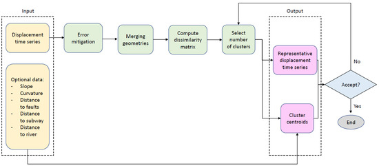
Figure 2.
Flowchart for the SARClust method.
Each step of the workflow will be explained in detail in the following subsections.
2.3.4. Displacement Time Series Error Mitigation
Displacement time series achieved from the PSI analysis may be affected by errors, such as movement at the reference point and residual atmospheric effects, which must be mitigated before the clustering analysis. SARClust uses an adaptation of the method presented in Notti et al. [15], where displacement time series are corrected based on displacements from PSs considered stable. PSs with large temporal coherence and average velocities between ±0.5 mm/year are considered stable, and the average of their displacement time series is removed from the time series of the remaining PSs, mitigating noise and regional effects. In SARClust, as average velocities are not available (non-linear displacements are considered in PSI analysis), the tool adjusts a regression model to each displacement time series and evaluates its slope. PSs are considered to have a stable behavior in case the slope is between ±0.5 mm/year. Similar to Notti et al. [15], the displacement time series of the stable PSs are averaged and removed from the time series of all PSs. This procedure is applied to the displacement time series of the ascending and of the descending passes, independently.
2.3.5. Merging of Ascending and Descending Data
The second step of the workflow is the merging of displacements from ascending and descending passes to obtain vertical and horizontal displacement time series at the same points and at the same epochs. Displacements along ascending and descending LOS are available for PSs at different locations. The inverse distance weighted (IDW) [38] method is used to interpolate displacement values in space. This enables the association of displacements from the two directions to all PSs. On the other hand, the observation epochs are also different for the two datasets. In this case, linear interpolation in time is performed to compute displacements from one direction to the epochs of the other one.
After the interpolations in space and time, vertical and horizontal displacements can be computed for all PSs and for all epochs. Displacements along LOS from ascending () and descending () passes are given by Equations (1) and (2), from Dentz et al. [39]:
where dV, dE and dN are vertical, easting and northing displacements, respectively, and are the incidence angles for ascending and descending passes and and are the satellite headings also for ascending and descending passes. Let β be the angle between LOS projection on the horizontal plane and the east–west direction, given by Equation (3):
where α is satellite orbit inclination and φ is latitude. The satellite headings for ascending and descending passes are given by Equations (4) and (5), respectively:
Let dH be the displacement along a direction of interest (DOI) on the horizontal plane and γ be the azimuth of the direction perpendicular to DOI. Easting and northing displacements are given by Equations (6) and (7):
Using Equations (4)–(7), Equations (1) and (2) can be written as in Equations (8) and (9):
From the equations above, dV and dH can be obtained through Equations (10) and (11):
SARClust uses Equations (10) and (11) to determine vertical and horizontal displacements. Nevertheless, due to the small sensitivity of InSAR data to displacements along north–south direction, only directions close to east–west must be considered.
In the particular case of downtown Lisbon, SARClust method was applied on the ascending and descending displacement time series of the PSs on buildings. Input data included the incidence angles and satellite orbit inclination to characterize the SAR image acquisition geometry. As the downtown area is mostly a flat area, ground-related horizontal displacements were not expected. However, there might be some movement on the hill slopes that flank the downtown area. Slope movement towards the downtown area would present an east–west orientation, approximately; therefore, this was the direction selected for the analysis of eventual horizontal displacements and γ was set to 0° in Equations (10) and (11). The merging of ascending and descending data led to the availability of vertical and east–west displacement time series at 974 PSs.
2.3.6. Dissimilarity Matrix
Vertical and horizontal displacement time series achieved from the previous step are the source data for the computation of the dissimilarity matrix. This matrix has as many rows and columns as PSs and each of its entries presents a value reflecting the dissimilarity between the displacement time series of the pair of PSs in the corresponding row/column. SARClust uses the distance between time series computed through the dynamic time warping (DTW) method as a dissimilarity measure. DTW considers the alignment between a reference and a query displacement time series (Figure 3) and computes the shortest cumulative path that connects them, which corresponds to the distance between the time series [32]. A constraint for the time interval in which matches are allowed is applied to avoid matches between displacements observed at distant epochs. This is achieved through a Sakoe and Chiba window with the duration of two epochs [40]. As DTW performance is affected by measurement noise [41], time series are filtered with a moving average before distance calculation.
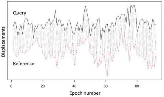
Figure 3.
Match of query and reference displacement time series in DTW, with a constraint window of two epochs.
Multivariate time series, considering both vertical and horizontal displacements at each PS, are used for the computation of the DTW distances. Low distance values correspond to low dissimilarities, meaning the pair of PSs being analyzed presents similar displacement time series in both vertical and horizontal directions.
2.3.7. Number of Clusters Selection
SARClust uses a hierarchical agglomerative clustering technique [31]. At the first step of the algorithm, each PS is considered to be an individual cluster and the clusters are iteratively aggregated to each other, based on their dissimilarities, until they are all merged into a single group. At each iteration, the pair of clusters presenting the lowest linkage distance (dissimilarity) is merged.
The tool enables the selection of one of three aggregation criteria when the clusters to be merged are formed by more than one PS: single linkage, complete linkage, and Ward method. In single linkage, the linkage distance between two clusters is the dissimilarity (i.e., the DTW distance) between the most similar displacement time series. On the other hand, complete linkage considers the less similar ones. Ward method aggregates the clusters in order to minimize the variance of the time series inside each group. For downtown Lisbon, complete linkage was selected as the aggregation criterion for the clustering as it leads to the creation of homogeneous clusters, while also being sensitive to the presence of outliers. The capability to isolate outliers is important in this case, as they may correspond to PSs with anomalies in their displacement time series.
The linkage distances provide information on the homogeneity of the displacement time series in each cluster at each iteration. Low linkage distances mean the clusters being merged have similar displacement time series. On the other hand, large linkage distances are observed when merging clusters with distinct displacement time series. Therefore, the number of clusters to analyze must be selected in order to assure the clusters merged in previous iterations are connected by low linkage distances. This can be evaluated through charts of absolute or relative linkage distances as a function of the number of clusters. An appropriate solution for the number of clusters to analyze is the number of clusters for which a large increase in absolute linkage distance is observed when a new pair of clusters is merged, which corresponds to a local maximum of the relative linkage distances. SARClust automatically identifies the lowest number of clusters corresponding to a local maximum of relative linkage distance and organizes the PSs accordingly. In case the selected clusters still present some variability, the user can evaluate the charts of linkage distances printed on the tool reports and manually select a larger number of clusters to analyze that will lead to cluster homogeneity.
In the case of Lisbon downtown, the analysis of the linkage distances led to the automatic organization of the PSs into three clusters, which was the lowest number of clusters being a local maximum of relative linkage distance (blue circle in Figure 4 and blue line in Figure 5). The displacement time series homogeneity in each cluster can be evaluated through a dendrogram (Figure 5), which is a tree-like graph of the linkage distances showing the evolution of the clusters throughout the iterations. The horizontal axis represents the clusters (individual PSs at the chart base), and the vertical axis presents the linkage distances. Long vertical lines correspond to large distances between the clusters being merged, which means the resulting cluster contains PSs with heterogeneous displacement time series. Figure 5 shows the three-cluster solution led to clusters that admitted variability in the displacement time series, as linkage distances connecting clusters from previous iterations were large. Therefore, a new number of clusters to analyze was manually selected to achieve larger homogeneity. The solution of 10 clusters was chosen, as it corresponded to another local maximum of relative distances (green dot in Figure 4 and green line in Figure 5). The dendrogram showed that linkage distances in previous iterations were low, meaning the displacement time series in each cluster were similar to each other and distinct from those of the other clusters. Therefore, the 10-cluster solution was adopted.
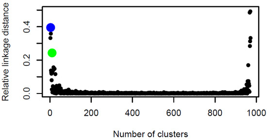
Figure 4.
Chart of relative linkage distance as a function of the number of clusters. Blue and green circles correspond to the automatic and manual solutions for the number of clusters to analyze, respectively.
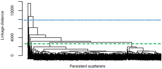
Figure 5.
Dendrogram showing the PS organization into clusters and the cutting of its branches corresponding to different solutions of number of clusters to analyze. The blue line corresponds to the automatic clustering solution and the green line represents the manual one.
Cluster centroids were computed for cumulative displacement and corrected altitude, both achieved through the PSI analysis. Furthermore, space variable quantities were also included (Figure 6). Raster images of slope and curvature were built using the EU-DEM, through Geographical Information System (GIS) software. Distance images to elements that might be related to ground instability were also considered, such as geological faults, underground infrastructures (subway network) and water lines (Tagus River) that were manually digitized from a geological map at the scale 1:50,000. These images were also achieved through GIS by computing the Euclidean distances between each pixel and those elements. For the sake of uniformity, all raster products were built with the spatial resolution of the DEM (25 m).
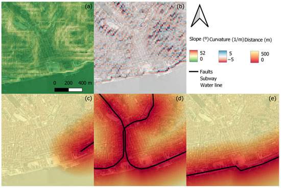
Figure 6.
Raster data for cluster centroids: (a) slope, (b) curvature, (c) distance to faults, (d) distance to the subway network and (e) distance to the water line. The background image is an aerial orthophotograph of the downtown area provided by the Portuguese National System for Geographical Information.
SARClust products, representative displacement time series and cluster centroids are provided for all cluster solutions and are made available in PDF and CSV formats.
3. Results and Discussion
3.1. Displacement Maps
Vertical and east–west displacements were analyzed through SARClust for the 974 PSs at the downtown area. Positive vertical displacement meant upward movement and negative values corresponded to downward movement. Positive horizontal displacement was movement towards the east, while negative values meant movement towards west. Vertical displacements ranged from −35.6 mm to 28.9 mm, and 93% of the PSs presented cumulative vertical displacement below 5 mm in the three years of the analysis. Horizontal displacements varied between 24.5 mm towards the west and 46.9 mm towards the east, and 82% of the points had cumulative horizontal displacements below 5 mm between 2015 and 2018 (Figure 7).
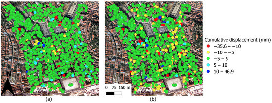
Figure 7.
(a) Vertical and (b) east–west cumulative displacement maps for the downtown area. The background image is an aerial orthophotograph of the downtown area provided by the Portuguese National System for Geographical Information.
3.2. Cluster Analysis
Two clustering solutions were achieved: the automatic solution of three clusters and the manual one of ten clusters. The spatial distribution of the clusters for both solutions is presented in Figure 8. Figure 9 shows the vertical and east–west displacement time series for all PSs in each cluster for the automatic solution. It was verified that the displacement time series in each cluster presented some variability, confirming the analysis of the dendrogram from Figure 5, which suggested a larger number of clusters should be analyzed.
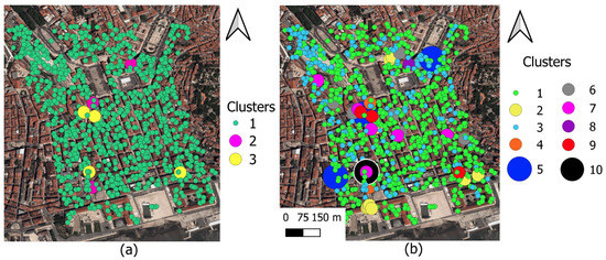
Figure 8.
Cluster spatial distribution for (a) automatic and (b) manual clustering solutions. The background image is an aerial orthophotograph of the downtown area provided by the Portuguese National System for Geographical Information.
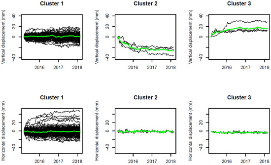
Figure 9.
Vertical and horizontal displacement time series for all PSs in each cluster (black lines), for the three-cluster solution. Green lines are the cluster-representative displacement time series.
For the 10-cluster solution, vertical and east–west displacement time series for the PSs in each cluster are presented in Figure 10 and Figure 11, respectively, together with the cluster representative time series. The clusters in this solution presented lower variability in the displacement time series than the three-cluster solution, for both directions. Nevertheless, minor variability was still observed. There were clusters in which a few time series presented deviations from the cluster main displacement trend at a small number of epochs or time series in the same cluster, presenting displacement discontinuities at different epochs. The cluster representative time series display the main displacement trends in each cluster.
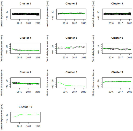
Figure 10.
Vertical displacement time series for all PSs in each cluster (black lines), for the ten-cluster solution. Green lines are the cluster-representative displacement time series.
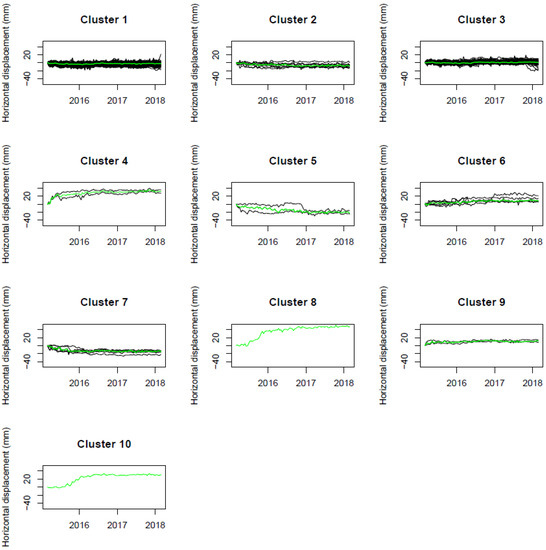
Figure 11.
Horizontal displacement time series for all PSs in each cluster (black lines), for the ten-cluster solution. Green lines are the cluster-representative displacement time series.
The displacement time series associated to the achieved 10 clusters showed that PSs were aggregated according to their displacement magnitude and movement direction. Clusters 1 and 3 presented small magnitude displacements for both vertical and east–west directions. The main difference between the two groups was that cluster 1 moved a few millimeters further west than cluster 3, as will be observed through the cluster centroids. Both clusters presented an oscillatory behavior in vertical displacement, moving up in summer and down in winter [42], which might be due to building thermal expansion (Figure 12). Cluster 2 presented displacements of a few millimeters up and towards the west, while the other clusters had displacements reaching the centimeter-level. Cluster 4 moved down and towards the east during 2015, when it stabilized. Clusters 5, 6 and 7 showed movement before 2018 and then stabilized. From these, cluster 5 presented uplift and displacement towards west. Clusters 6 and 7 both moved downward, but while cluster 6 moved east, cluster 7 went west. Cluster 8 moved down and east in 2015, stabilizing after that. Clusters 9 and 10 both moved up and towards the east; however, while cluster 9 stabilized in 2015, cluster 10 only stabilized in 2016 and the displacement magnitude for cluster 10 was larger than for cluster 9. By the end of the study period, there were no clusters presenting movement.
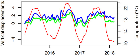
Figure 12.
Comparison between vertical displacement time series representative of clusters 1 (green) and 3 (blue) and monthly temperature (red).
Cluster interpretation was assisted by the centroids computed based on PSI estimated variables and spatial variable quantities (Table 1). Clusters 1 and 3 together contained 96.7% of the PSs, while the remaining clusters accounted only for 32 points. Altitude centroid informed whether the clusters were mainly located on the downtown area (lower values) or on the flanking hillslopes. Vertical and horizontal displacements provided information on the movement direction. Regarding terrain configuration, according to Rosi et al. [43], landslides tend to occur for slopes larger than 10° and at slightly concave surfaces (positive curvature). Table 1 shows that clusters 4 and 8, both presenting centimeter-level displacements, were located at areas with those characteristics. PSs in these clusters moved down and towards the east, which was compatible to downslope movement and suggested that the observed displacements might be related to ground instability. Clusters 5, 7, 9 and 10 also presented centimeter-level displacements and were associated with concave surfaces. However, their PSs were located on approximately flat areas or moved upwards, which suggested their displacements might not be related to the slope, but to the buildings themselves. Among the distance centroids, the distance to the subway showed the strongest association to displacements, as the four clusters with larger displacement magnitude (4, 5, 8 and 10) were located less than 50 m away from the subway line, in average (Figure 13). Nevertheless, these subway segments were built several years before the study period. Clusters 5 and 8 had PSs close to a subway segment built in 1966 and clusters 4, 5 and 10 contained PSs close to segments from 1998 and 2007. Vibration tests at buildings in that area revealed that vibrations caused by the subway passage did not affect the structures [44]. Therefore, despite the clusters’ proximity to the subway, it was not likely the displacements had been influenced by the underground infrastructure. The data did not suggest any relationship between the clusters and the distances to faults or to the river. No relationship was identified between clusters 2 and 6 and the centroids.

Table 1.
Percentage of PSs in each cluster and cluster centroids.
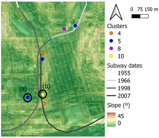
Figure 13.
Spatial relationship between PSs from clusters 4, 5, 8 and 10, slope and inauguration dates of subway segments. The background image is an aerial orthophotograph of the downtown area provided by the Portuguese National System for Geographical Information.
3.3. Visual Inspection
Buildings with PSs belonging to the largest displacements clusters were visually inspected. The objective was to verify whether there were any signs of damage that could be related to the observed displacements. Many of these buildings presented cracks at their façades or at stonework, while others revealed signs of recent maintenance activities, such as painting, and no pathologies were visible. Figure 14 shows pictures of façades from the buildings corresponding to the PSs inside black circumferences in Figure 13, where cracks were identified, showing the presence of damages possibly related to the observed displacements.
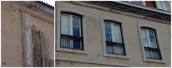
Figure 14.
Examples of cracks on buildings associated to centimeter-level displacement clusters, in August 2019. Pictures (a,b) correspond to PSs (a,b) in Figure 13, respectively.
3.4. Comparison to Other Radar Interpretation Tools
SARClust uses a hierarchical clustering approach to aggregate PSs according to the similarities among their displacement time series, considering vertical and horizontal directions simultaneously. The proposed method is independent of the nature of the observed displacements and of the SAR image sensor, as its application only requires the availability of displacement time series. Auxiliary variables can be used to assist cluster interpretation, but they are not mandatory as in other radar interpretation methods [16]. The delivery of vertical and horizontal displacements makes SARClust products easily interpretable by InSAR non-experts.
Hierarchical clustering provides information on the displacement time series similarity in each cluster, which assists the selection of the number of clusters to analyze, unlike partitioning methods, such as those used in Milone and Scepi [11], where a less informed decision needs to be made. DTW is a frequently used technique to compare time series. Although some authors recommend against its usage to analyze InSAR displacement time series due to the noise affecting the data [41], it was verified in this study that the low pass filtering of the time series was effective, as it led to the formation of homogeneous clusters.
The analysis performed for the case study showed the proposed method was not very sensitive to displacement changes at a small number of epochs in long time series. This might be overcome in future work by using representation techniques which organize time series into small segments, reducing their dimensionality and increasing the tool capability to detect those deviations.
A frequent strategy for radar interpretation is the usage of libraries of expected deformation models and the application of sequences of statistical tests to classify displacement time series into those models [13,14]. In order to assess the performance of SARClust, the vertical displacement time series from Figure 10 were analyzed using the tool PS-Time, freely available from the University of Bologna, Italy [13]. PS-Time was run using 0.01 as level of significance for the statistical tests and the 974 displacement time series were classified into six classes: uncorrelated (class 0), linear (class 1), quadratic (class 2), bilinear (class 3), discontinuous with constant velocity (class 4) and discontinuous with variable velocity (class 5). Table 2 presents the contingency table between SARClust clusters and PS-Time classes.
Table 2.
Contingency table between SARClust clusters and PS-Time classes.
The comparison showed displacement time series classified as uncorrelated and as linear, i.e., time series that did not present sudden changes in displacements, were mainly attributed to clusters 1 and 3. The results from both tools agreed with each other, as clusters 1 and 3 were those tendentially stable, having small magnitude displacements. The quadratic class was associated also with clusters 1 and 3. This class of time series is characterized by a smooth change in displacement values, without a breaking point. Therefore, the inclusion of these displacement time series into the tendentially stable clusters was also appropriate. Displacement time series having a breaking point between segments of different velocities, classified as bilinear, were scattered through several clusters according to their displacement magnitude. Time series corresponding to small displacement magnitudes were attributed to clusters 1, 2 and 3, while those associated with large displacement magnitudes were spread through clusters 4, 5, 6, 7 and 9 according to the displacement magnitudes and directions that characterize each cluster. Figure 10 shows each of these clusters contained time series presenting movement upward or downward during the first years of the analysis and then stabilized. This result is consistent with the presence of bilinear time series in these clusters. All time series in clusters 4 and 9 belong to this class. Discontinuous with constant velocity time series are characterized by presenting linear behavior which is discontinued by a sudden change in displacement value at a certain epoch. Time series in this class were mainly set to cluster 7, which presented a stable trend followed by a sudden movement downward before becoming stable again. Similar trends were observed for PSs at clusters 2, 3 and 6, which were also associated with discontinuous time series. Therefore, the agreement between the results from both tools was also observed for this type of time series. The last class considered in PS-Time, discontinuous with variable velocity, is similar to the previous one, except that the segments of the time series before and after the change in displacement have different velocities. Time series with this behavior were spread through clusters 1, 3, 5, 6, 8 and 10 according to each cluster displacement magnitude and direction. Clusters 8 and 10 were formed by isolated PSs whose time series belonged to this class. Cluster 8 showed a stable behavior followed by a sudden movement downward that slowed down. Cluster 10 presented low velocity upward movement which suffered an acceleration and then stabilized. Therefore, the results from the cluster analysis also agreed with the PS-Time classification is this case.
In general, there was agreement between the results from the two tools. However, there were a few exceptions, such as tendentially stable clusters 1 and 3 presenting bilinear or discontinuous time series, or clusters associated to movement, such as clusters 6 and 7, containing uncorrelated and linear time series. These unconformities were due to the influence of displacement magnitude on the DTW. If displacement magnitude was similar for a pair of displacement time series, they tended to be aggregated into the same cluster regardless of the type of transition (smooth or sudden) between different types of movement. On the other hand, the attribution of time series classified with the same type of anomaly to different clusters demonstrated SARClust capability to distinguish between time series with different displacement magnitudes and directions, which are useful information for structure monitoring and assist the characterization of the eventual detected damage.
SARClust provided a summary of the distinct behaviors of the structures at the study area, which allowed the identification of damage location (PS coordinates), extension (clusters of PSs with similar displacements), degree (displacement magnitude) and evolution (displacement time series). This information enables structure experts to plan other monitoring activities more efficiently—for example, visual inspections or other in situ methods—which depend on field work and have associated ecological and economic costs. Therefore, SARClust contributes to turning the monitoring activities more sustainable.
3.5. Computational Performance
Hierarchical clustering and DTW are computationally demanding algorithms [45]. In order to improve the tool processing time, the computation of the dissimilarity matrix in R© software was parallelized [37]. The dataset analyzed in this study took 11 min to be processed in a laptop with 2.40 GHz CPU, 8 GB of RAM and four cores.
4. Conclusions
In this study, a new tool for the radar interpretation of PSI displacement time series was proposed and its performance was evaluated in the context of structure monitoring at an urban area. The global, frequent and free availability of SAR images has turned PSI into an interesting technique to continuously monitor structure behavior. However, the large amount of data provided by this technology and the measurement noise make the detection of damage signs in structures difficult. The SARClust tool aggregates PSs in clusters, enabling the identification of spatiotemporal patterns in displacements and the identification of eventual anomalies possibly related to structure damages.
The tool was tested for downtown Lisbon, Portugal, a cultural heritage site almost 270 years old. Buildings presenting centimeter-level displacements were detected through the proposed method and visual inspections confirmed the presence of damage. A relationship between displacements and steep slopes was observed for some clusters. The results showed that the observed displacements stopped before February 2018.
The method shows low sensitivity to detect small changes in large displacement time series. This issue will be addressed in future work through the usage of different distance measures between time series or by applying techniques to reduce time series dimension. For future work, the authors also intend to combine the proposed method with machine learning in order to automatically identify clusters that may potentially pose a threat to structural safety.
In conclusion, the proposed tool is effective in detecting anomalies in InSAR displacement time series associated to cultural heritage buildings, contributing to a more sustainable management of these areas, and with ecological and economic benefits since field work is reduced, leading to more resilient and safe cities.
Author Contributions
Conceptualization, D.R., A.P.F., C.A., J.V.L. and A.F.; methodology, D.R.; software, D.P. and D.R.; validation, D.R.; formal analysis, D.R.; investigation, D.R.; resources, D.R., A.P.F., J.V.L. and A.F.; data curation, D.P. and D.R.; writing—original draft preparation, D.R.; writing—review and editing, D.R., A.P.F., D.P., C.A., J.V.L. and A.F.; visualization, D.R.; supervision, A.P.F., D.P., J.V.L. and A.F.; project administration, A.F. and A.P.F.; funding acquisition, D.R., A.P.F., J.V.L. and A.F. All authors have read and agreed to the published version of the manuscript.
Funding
This research was funded by Fundação para a Ciência e a Tecnologia grant number SFRH/BD/115882/2016.
Institutional Review Board Statement
Not applicable.
Informed Consent Statement
Not applicable.
Data Availability Statement
The data presented in this study are available on request from the corresponding author. The data are not publicly available due to being proprietary and may be available only with authorization from the National Laboratory for Civil Engineering Board of Directors. Remotely sensed data are downloadable from the corresponding sites.
Acknowledgments
The authors would like to thank Maria João Henriques (LNEC) for providing the computational resources for PSI analysis, the European Space Agency for the Sentinel-1 images, the European Environmental Agency for the DEM and the Portuguese General-Directorate of the Territory for the aerial orthophotographs.
Conflicts of Interest
The authors declare no conflict of interest.
References
- Aslan, G.; Cakir, Z.; Ergintav, S.; Lasserre, C.; Renard, F. Analysis of Secular Ground Motions in Istanbul from a Long-Term InSAR Time-Series (1992–2017). Remote Sens. 2018, 10, 408. [Google Scholar] [CrossRef]
- Heleno, S.I.N.; Oliveira, L.G.S.; Henriques, M.J.; Falcão, A.P.; Lima, J.N.P.; Cooksley, G.; Ferretti, A.; Fonseca, A.M.; Lobo-Ferreira, J.P.; Fonseca, J.F.B.D. Persistent Scatterers Interferometry Detects and Measures Ground Subsidence in Lisbon. Remote Sens. Environ. 2011, 115, 2152–2167. [Google Scholar] [CrossRef]
- Osmanoğlu, B.; Dixon, T.H.; Wdowinski, S.; Cabral-Cano, E.; Jiang, Y. Mexico City Subsidence Observed with Persistent Scatterer InSAR. Int. J. Appl. Earth Obs. Geoinf. 2011, 13, 1–12. [Google Scholar] [CrossRef]
- Yao, G.; Ke, C.Q.; Zhang, J.; Lu, Y.; Zhao, J.; Lee, H. Surface Deformation Monitoring of Shanghai Based on ENVISAT ASAR and Sentinel-1A Data. Environ. Earth Sci. 2019, 78, 225. [Google Scholar] [CrossRef]
- Qin, Y.; Perissin, D. Monitoring Ground Subsidence in Hong Kong via Spaceborne Radar: Experiments and Validation. Remote Sens. 2015, 7, 10715–10736. [Google Scholar] [CrossRef]
- Lanari, R.; Lundgren, P.; Manzo, M.; Casu, F. Satellite Radar Interferometry Time Series Analysis of Surface Deformation for Los Angeles, California. Geophys. Res. Lett. 2004, 31, L23613. [Google Scholar] [CrossRef]
- Stramondo, S.; Bozzano, F.; Marra, F.; Wegmuller, U.; Cinti, F.R.; Moro, M.; Saroli, M. Subsidence Induced by Urbanisation in the City of Rome Detected by Advanced InSAR Technique and Geotechnical Investigations. Remote Sens. Environ. 2008, 112, 3160–3172. [Google Scholar] [CrossRef]
- Lanari, R.; Berardino, P.; Bonano, M.; Casu, F.; Manconi, A.; Manunta, M.; Manzo, M.; Pepe, A.; Pepe, S.; Sansosti, E.; et al. Surface Displacements Associated with the L’Aquila 2009 Mw 6.3 Earthquake (Central Italy): New Evidence from SBAS-DInSAR Time Series Analysis. Geophys. Res. Lett. 2010, 37, L20309. [Google Scholar] [CrossRef]
- Cigna, F.; Tapete, D.; Casagli, N. Semi-Automated Extraction of Deviation Indexes (DI) from Satellite Persistent Scatterers Time Series: Tests on Sedimentary Volcanism and Tectonically-Induced Motions. Nonlinear Process. Geophys. 2012, 19, 643–655. [Google Scholar] [CrossRef]
- Cigna, F.; del Ventisette, C.; Liguori, V.; Casagli, N. Advanced Radar-Interpretation of InSAR Time Series for Mapping and Characterization of Geological Processes. Nat. Hazards Earth Syst. Sci. 2011, 11, 865–881. [Google Scholar] [CrossRef]
- Milone, G.; Scepi, G. A Clustering Approach for Studying Ground Deformation Trends in Campania Region through PS-InSARTM Time Series Analysis. J. Appl. Sci. 2011, 11, 610–620. [Google Scholar] [CrossRef]
- Bakon, M.; Oliveira, I.; Perissin, D.; Sousa, J.J.; Papco, J. A Data Mining Approach for Multivariate Outlier Detection in Postprocessing of Multitemporal InSAR Results. IEEE J. Sel. Top. Appl. Earth Obs. Remote. Sens. 2017, 10, 2791–2798. [Google Scholar] [CrossRef]
- Berti, M.; Corsini, A.; Franceschini, S.; Iannacone, J.P. Automated Classification of Persistent Scatterers Interferometry Time Series. Nat. Hazards Earth Syst. Sci. 2013, 13, 1945–1958. [Google Scholar] [CrossRef]
- Chang, L.; Hanssen, R.F. A Probabilistic Approach for InSAR Time-Series Postprocessing. IEEE Trans. Geosci. Remote Sens. 2016, 54, 421–430. [Google Scholar] [CrossRef]
- Notti, D.; Calò, F.; Cigna, F.; Manunta, M.; Herrera, G.; Berti, M.; Meisina, C.; Tapete, D.; Zucca, F. A User-Oriented Methodology for DInSAR Time Series Analysis and Interpretation: Landslides and Subsidence Case Studies. Pure Appl. Geophys. 2015, 172, 3081–3105. [Google Scholar] [CrossRef]
- Tomás, R.; Pagán, J.I.; Navarro, J.A.; Cano, M.; Pastor, J.L.; Riquelme, A.; Cuevas-González, M.; Crosetto, M.; Barra, A.; Monserrat, O.; et al. Semi-Automatic Identification and Pre-Screening of Geological–Geotechnical Deformational Processes Using Persistent Scatterer Interferometry Datasets. Remote Sens. 2019, 11, 1675. [Google Scholar] [CrossRef]
- van de Kerkhof, B.; Pankratius, V.; Chang, L.; van Swol, R.; Hanssen, R.F. Individual Scatterer Model Learning for Satellite Interferometry. IEEE Trans. Geosci. Remote Sens. 2020, 58, 1273–1280. [Google Scholar] [CrossRef]
- Fadhillah, M.F.; Achmad, A.R.; Lee, C.W. Integration of InSAR Time-Series Data and GIS to Assess Land Subsidence along Subway Lines in the Seoul Metropolitan Area, South Korea. Remote Sens. 2020, 12, 3505. [Google Scholar] [CrossRef]
- Mirmazloumi, S.M.; Gambin, A.F.; Wassie, Y.; Barra, A.; Palamà, R.; Crosetto, M.; Monserrat, O.; Crippa, B. InSAR Deformation Time Series Classification Using a Convolutional Neural Network. Int. Arch. Photogramm. Remote Sens. Spat. Inf. Sci. 2022, 43, 307–312. [Google Scholar] [CrossRef]
- Wang, L.; Li, S.; Teng, C.; Jiang, C.; Li, J.; Li, Z.; Huang, J. Automatic-Detection Method for Mining Subsidence Basins Based on InSAR and CNN-AFSA-SVM. Sustainability 2022, 14, 13898. [Google Scholar] [CrossRef]
- Anantrasirichai, N.; Biggs, J.; Albino, F.; Hill, P.; Bull, D. Application of Machine Learning to Classification of Volcanic Deformation in Routinely Generated InSAR Data. J. Geophys. Res. Solid Earth 2018, 123, 6592–6606. [Google Scholar] [CrossRef]
- Brengman, C.M.J.; Barnhart, W.D. Identification of Surface Deformation in InSAR Using Machine Learning. Geochem. Geophys. Geosystems 2021, 22, e2020GC009204. [Google Scholar] [CrossRef]
- Maubant, L.; Pathier, E.; Daout, S.; Radiguet, M.; Doin, M.P.; Kazachkina, E.; Kostoglodov, V.; Cotte, N.; Walpersdorf, A. Independent Component Analysis and Parametric Approach for Source Separation in InSAR Time Series at Regional Scale: Application to the 2017–2018 Slow Slip Event in Guerrero (Mexico). J. Geophys. Res. Solid Earth 2020, 125, e2019JB018187. [Google Scholar] [CrossRef]
- Rouet-Leduc, B.; Jolivet, R.; Dalaison, M.; Johnson, P.A.; Hulbert, C. Autonomous Extraction of Millimeter-Scale Deformation in InSAR Time Series Using Deep Learning. Nat. Commun. 2021, 12, 6480. [Google Scholar] [CrossRef]
- Zhao, Z.; Wu, Z.; Zheng, Y.; Ma, P. Recurrent Neural Networks for Atmospheric Noise Removal from InSAR Time Series with Missing Values. ISPRS J. Photogramm. Remote Sens. 2021, 180, 227–237. [Google Scholar] [CrossRef]
- Sorkhabi, O.M.; Nejad, A.S.; Khajehzadeh, M. Evaluation of Isfahan City Subsidence Rate Using InSAR and Artificial Intelligence. KSCE J. Civ. Eng. 2022, 26, 2901–2908. [Google Scholar] [CrossRef]
- Martin, G.; Hooper, A.; Wright, T.J.; Selvakumaran, S. Blind Source Separation for MT-InSAR Analysis with Structural Health Monitoring Applications. IEEE J. Sel. Top. Appl. Earth Obs. Remote. Sens. 2022, 15, 7605–7618. [Google Scholar] [CrossRef]
- Gualandi, A.; Liu, Z. Variational Bayesian Independent Component Analysis for InSAR Displacement Time-Series with Application to Central California, USA. J. Geophys. Res. Solid Earth 2021, 126, e2020JB020845. [Google Scholar] [CrossRef]
- Chen, Y.; He, Y.; Zhang, L.; Chen, Y.; Pu, H.; Chen, B.; Gao, L. Prediction of InSAR Deformation Time-Series Using a Long Short-Term Memory Neural Network. Int. J. Remote Sens. 2021, 42, 6921–6944. [Google Scholar] [CrossRef]
- Radman, A.; Akhoondzadeh, M.; Hosseiny, B. Integrating InSAR and Deep-Learning for Modeling and Predicting Subsidence over the Adjacent Area of Lake Urmia, Iran. GIScience Remote Sens. 2021, 58, 1413–1433. [Google Scholar] [CrossRef]
- Hair, J.F.; Black, W.C.; Babin, B.J.; Anderson, R.E. Multivariate Data Analysis, 7th ed.; Prentice Hall: Upper Saddle River, NJ, USA, 2009. [Google Scholar]
- Berndt, D.; Clifford, J. Using Dynamic Time Warping to Find Patterns in Time Series. In Workshop on Knowledge Discovery in Databases; KDD Workshop: Seattle, WA, USA, 1994; Volume 10, pp. 359–370. [Google Scholar]
- Perissin, D.; Wang, Z.; Wang, T. The SARPROZ InSAR Tool for Urban Subsidence/Manmade Structure Stability Monitoring in China. In Proceedings of the 34th International Symposium for Remote Sensing of the Environment (ISRSE), Sydney, Australia, 10–15 April 2011; p. 4. [Google Scholar]
- Milillo, P.; Perissin, D.; Salzer, J.T.; Lundgren, P.; Lacava, G.; Milillo, G.; Serio, C. Monitoring Dam Structural Health from Space: Insights from Novel InSAR Techniques and Multi-Parametric Modeling Applied to the Pertusillo Dam Basilicata, Italy. Int. J. Appl. Earth Obs. Geoinf. 2016, 52, 221–229. [Google Scholar] [CrossRef]
- CNES. Orfeo ToolBox. Available online: https://www.orfeo-toolbox.org/ (accessed on 29 September 2020).
- Zouhal, L.M.; Denoeux, T. An Evidence-Theoretic k-NN Rule with Parameter Optimization. IEEE Trans. Syst. Man Cybern. Part C 1998, 28, 263–271. [Google Scholar] [CrossRef]
- R Core Team. R: A Language and Environment for Statistical Computing; R Foundation for Statistical Computing: Vienna, Austria, 2018; Available online: http://www.r-project.org/ (accessed on 29 August 2019).
- Bartier, P.M.; Keller, C.P. Multivariate Interpolation to Incorporate Thematic Surface Data Using Inverse Distance Weighting (IDW). Comput. Geosci. 1996, 22, 795–799. [Google Scholar] [CrossRef]
- Dentz, F.; van Halderen, L.; Boudewijn, P.; Esfahany, S.S.; Slobbe, C.; Wortel, T. “POSEIDON” on the Potential of Satellite Radar Interferometry for Monitoring Dikes of the Netherlands—A Technical Feasibility Study; Delft University of Technology: Delft, The Netherlands, 2006. [Google Scholar]
- Sakoe, H.; Chiba, S. Dynamic Programming Algorithm Optimization for Spoken Word Recognition. IEEE Trans. Acoust. 1978, 26, 43–49. [Google Scholar] [CrossRef]
- Romano, E.; Scepi, G. Integrating Time Alignment and Self-Organizing Maps for Classifying Curves. In Proceedings of the Knowledge Extraction and Modeling Workshop, Capri, Italy, 4–6 September 2006; pp. 1–5. [Google Scholar]
- TWC Product and Technology LLC. Lisbon, Lisbon, Portugal Weather History. Available online: https://www.wunderground.com/ (accessed on 12 February 2023).
- Rosi, A.; Tofani, V.; Tanteri, L.; Tacconi Stefanelli, C.; Agostini, A.; Catani, F.; Casagli, N. The New Landslide Inventory of Tuscany (Italy) Updated with PS-InSAR: Geomorphological Features and Landslide Distribution. Landslides 2018, 15, 5–19. [Google Scholar] [CrossRef]
- LNEC. Estudo Sobre a Fissuração Em Revestimentos de Paredes No Edifício Ivens Arte; Laboratório Nacional de Engenharia Civil, Proc. 0803/121/22265. Report No. 162/2020–DED/NRI; Portuguese National Laboratory for Civil Engineering: Lisbon, Portugal, 2020. [Google Scholar]
- Aghabozorgi, S.; Shirkhorshidi, A.S.; Wah, T.Y. Time-Series Clustering—A Decade Review. Inf. Syst. 2015, 53, 16–38. [Google Scholar] [CrossRef]


Disclaimer/Publisher’s Note: The statements, opinions and data contained in all publications are solely those of the individual author(s) and contributor(s) and not of MDPI and/or the editor(s). MDPI and/or the editor(s) disclaim responsibility for any injury to people or property resulting from any ideas, methods, instructions or products referred to in the content. |
© 2023 by the authors. Licensee MDPI, Basel, Switzerland. This article is an open access article distributed under the terms and conditions of the Creative Commons Attribution (CC BY) license (https://creativecommons.org/licenses/by/4.0/).